A Risk Ratio Comparison of $l_{0}$ and $l_{1}$ Penalized Regression

Abstract

There has been an explosion of interest in using $l_{1}$-regularization in place of $l_{0}$-regularization for feature selection. We present theoretical results showing that while $l_{1}$-penalized linear regression never outperforms $l_{0}$-regularization by more than a constant factor, in some cases using an $l_{1}$ penalty is infinitely worse than using an $l_{0}$ penalty. We also show that the “optimal” $l_{1}$ solutions are often inferior to $l_{0}$ solutions found using stepwise regression.

We also compare algorithms for solving these two problems and show that although solutions can be found efficiently for the $l_{1}$ problem, the “optimal” $l_{1}$ solutions are often inferior to $l_{0}$ solutions found using greedy classic stepwise regression. Furthermore, we show that solutions obtained by solving the convex $l_{1}$ problem can be improved by selecting the best of the $l_{1}$ models (for different regularization penalties) by using an $l_{0}$ criterion. In other words, an approximate solution to the right problem can be better than the exact solution to the wrong problem.

Keywords: Variable Selection, Streaming Feature Selection, Regularization, Stepwise Regression, Submodularity

1 Introduction

In the past decade, a rich literature has been developed using $l_{1}$-regularization for linear regression including Lasso (Tib96), LARS (Efron+04), fused lasso (Tib+05), elastic net (ZouH05), grouped lasso (YuanL06), adaptive lasso (Zou06), and relaxed lasso (Mein07). These methods, like the $l_{0}$-penalized regression methods which preceded them (Aka74; Schwarz78; FosterG94), address variable selection problems in which there is a large set of potential features, only a few of which are likely to be helpful. This type of sparsity is common in machine learning tasks, such as predicting disease based on thousands of genes, or predicting the topic of a document based on the occurrences of hundreds of thousands of words.

$l_{1}$-regularization is popular because, unlike the $l_{0}$ regularization historically used for feature selection in regression problems, the $l_{1}$ penalty gives rise to a convex problem that can be solved efficiently using convex optimization methods. $l_{1}$ methods have given reasonable results on a number of data sets, but there has been no careful analysis of how they perform when compared to $l_{0}$ methods. This paper provides a formal analysis of the two methods, and shows that $l_{1}$ can give arbitrarily worse models. We offer some intuition as to why this is the case – $l_{1}$ shrinks coefficients too much and does not zero out enough of them – and suggest how to use an $l_{0}$ penalty with $l_{1}$ optimization.

We study the problem of selecting predictive features from a large feature space. We assume the classic normal linear model rCl+rCl y& = Xβ+ ϵ ϵ ∼ N_n(0,σ^2 I_n) with $n$ observations $\mathbf{y}=(y_{1},\ldots,y_{n})^{\prime}$ and $p$ features $\mathbf{x}_{1},\ldots,\mathbf{x}_{p}$, where $\mathbf{X}=(\mathbf{x}_{1},\ldots,\mathbf{x}_{p})$ is an $n\times p$ “design matrix” of features, $\boldsymbol{\beta}=(\beta_{1},\ldots,\beta_{p})^{\prime}$ is the coefficient parameters, and error $\boldsymbol{\varepsilon}\sim N(\mathbf{0},\sigma^{2}I_{n})$.

We expect most of the elements of $\beta$ to be 0. Hence, generating good predictions requires identifying the small subset of predictive features. This standard linear model proliferates the statistics and machine learning literature. In modern applications, $p$ can approach millions, making the selection of an appropriate subset of these features essential for prediction. The size and scope of these problems raise concerns about both the speed and statistical robustness of the selection procedure. Namely, it must be fast enough to be computationally feasible and must find signal without over-fitting the data.

The traditional statistical approach to this problem, namely, the $l_{0}$ regularization problem, finds an estimator that minimizes the $l_{0}$ penalized sum of squared errors,

$${\arg\min}_{\boldsymbol{\beta}}\left\{\|\mathbf{y}-\mathbf{X}\boldsymbol{\beta}\|^{2}+\lambda_{0}\|\boldsymbol{\beta}\|_{l_{0}}\right\},$$ (1)

where $\|\boldsymbol{\beta}\|_{l_{0}}=\sum_{i=1}^{p}I_{\{\beta_{i}\neq 0\}}$ counts the number of nonzero coefficients. However, this problem is NP-hard (Nata95). A tractable problem relaxes the $l_{0}$ penalty to the $l_{1}$ norm, $\|\boldsymbol{\beta}\|_{l_{1}}=\sum_{i=1}^{p}|\beta_{i}|$, and seeks

$${\arg\min}_{\boldsymbol{\beta}}\left\{\|\mathbf{y}-\mathbf{X}\boldsymbol{\beta}\|^{2}+\lambda_{1}\|\boldsymbol{\beta}\|_{l_{1}}\right\},$$ (2)

This is known as the $l_{1}$-regularization problem (Tib96), which is convex. This problem can be solved efficiently using a variety of methods (Tib96; Efron+04; CanT07).

We assess our models using the predictive risk function (1) rCcCl R(β, ^β) & = E_β ∥ ^y- E(y—X)∥_2^2 = E_β ∥X^β- Xβ∥_2^2. We are interested in the ratios of the risks of the estimates provided by these two criteria. Unlike risk functions, predictive risk measures the relevant prediction error on future observations, ignoring irreducible variance. Smaller risks imply better expected prediction performance. It is an ideal metric to analyze testing error or out-of-sample errors when the parameter distribution is assumed to be known. Recent literature has focused on selection consistency: whether or not the true variable can be identified in the limit. However, in real application, due to ubiquitous multicollinearity, predictors are hard to separate as “true” and “false”. Here, we focus on predictive accuracy and advocate the concept of predictive risk.

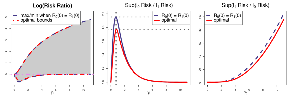
Our first result in this paper, given below as Theorems 1 and 2 in Section 2, is that $l_{0}$ estimates provide more accurate predictions than $l_{1}$ estimates do, in the sense of minimax risk ratios. This is illustrated in Figure 1. Proofs of these theorems are in Appendix A.

• $\inf_{\gamma_{0}}\sup_{\boldsymbol{\beta}}\frac{R(\boldsymbol{\beta},\hat{\boldsymbol{\beta}}_{l_{0}}(\gamma_{0}))}{R(\boldsymbol{\beta},\hat{\boldsymbol{\beta}}_{l_{1}}(\gamma_{1}))}$ is bounded by a small constant; furthermore, it is close to one for most $\gamma_{1}$s, especially for large $\gamma_{1}$s, which are mostly used in sparse systems.

• $\inf_{\gamma_{1}}\sup_{\boldsymbol{\beta}}\frac{R(\boldsymbol{\beta},\hat{\boldsymbol{\beta}}_{l_{1}}(\gamma_{1}))}{R(\boldsymbol{\beta},\hat{\boldsymbol{\beta}}_{l_{0}}(\gamma_{0}))}$ tends to infinity quadratically; in an extremely sparse system, the $l_{1}$ estimate may perform arbitrarily badly.

• $R(\boldsymbol{\beta},\hat{\boldsymbol{\beta}}_{l_{1}}(\gamma_{1}))$ is more likely to have a larger risk than $R(\boldsymbol{\beta},\hat{\boldsymbol{\beta}}_{l_{0}}(\gamma_{0}))$ does. backgroundcolor=blue!20!white,inline, bordercolor=red]how is “more likely” defined?

Figure 1: Left: The gray area shows the feasible region for the risk ratios–the log risk-ratio is above zero when $l_{0}$ produces a better fit. The graph shows that most of the time $l_{0}$ is better. The actual estimators being compared are those that have the same risk at $\beta=0$, i.e., $R(0,\hat{\beta}_{l_{0}}(\gamma_{0}))=R(0,\hat{\beta}_{l_{1}}(\gamma_{1}))$. Middle: This graph traces out the bottom envelope of the left hand graph (but takes the reciprocal risk ratio and no longer uses the logarithm scale). The dashed blue line displays $\sup_{\beta}{R(\beta,\hat{\beta}_{l_{0}}(\gamma_{0}))}/{R(\beta,\hat{\beta}_{l_{1}}(\gamma_{1}))}$ for $\gamma_{0}$ calibrated to have the same risk at zero as $\gamma_{1}$. This maximum ratio tends to 1 when $\gamma_{1}\rightarrow 0$ (the saturated case) or $\infty$ (the sparse case). With an optimal choice of $\gamma_{0}$, $\inf_{\gamma_{0}}\sup_{\beta}{R(\beta,\hat{\beta}_{l_{0}}(\gamma_{0}))}/{R(\beta,\hat{\beta}_{l_{1}}(\gamma_{1}))}$ (solid red line) behaves similarly. Specifically, the supremum over $\gamma_{1}$ is bounded by 1.8. Right: This graph traces out the upper envelopes of the left hand graph on a normal scale. When $\gamma_{0}\rightarrow\infty$, $\sup_{\beta}{R(\beta,\hat{\beta}_{l_{1}}(\gamma_{1}))}/{R(\beta,\hat{\beta}_{l_{0}}(\gamma_{0}))}$ tends to $\infty$, for both $\gamma_{1}$ that is calibrated at $\beta=0$ and that minimizes the maximum risk ratio.

A detailed discussion on the risk ratios will be presented in Section 2, along with a discussion of other advantages of $l_{0}$ regularization. Our other comparative results include showing that applying the $l_{0}$ criterion on an $l_{1}$ subset searching path can find the best performing model (Section 2.3.1) and running stepwise regression and Lasso on a reduced NP hard example shows that stepwise regression gives better solutions (Section 2.3.2).

backgroundcolor=blue!20!white,inline, bordercolor=red]Check all assumptions or remove. We compare $l_{0}$ vs. $l_{1}$ penalties under three assumptions about the structure of the feature matrix $X$: independence, incoherence (near independence) and NP-hard. For independence, we find provide the theoretical results mentioned above. For near independence, we find that $l_{1}$ penalized regression followed by $l_{0}$ outperforms $l_{1}$ selection. For the NP-hard case, we find that if one could do the search, then the risk ratio could be arbitrarily bad for $l_{1}$ relative to $l_{0}$.

2 Risk Ratio Comparison

We assess our models using the predictive risk function (1) rCcCl R(β,^β) & = E_β ∥ ^y- E(y—X) ∥_2^2 = E_β ∥X^β- Xβ∥_2^2.

This is the relevant component after decomposing the expected squared error loss from predicting a new observation. This is clear from the following standard decomposition. For increased generality, let $\mathbb{E}[y]=\eta]$ and $\mathbf{H}_{\mathbf{X}}$ be the projection onto the column space of $\mathbf{X}$. Then rCl E∥y^* - X^β∥^2 & = E∥y^*-η∥^2 + E∥η- H_Xη∥^2 + E∥H_Xη- X^β∥^2
= ⏟n σ^2_common error + ⏟∥(I- H_X)η∥^2_wrong $\mathbf{X}$ + ⏟E∥H_Xη- X^β∥^2_predictive risk

The first term, common error, is unavoidable, regardless of the method being used. All methods we consider, namely linear methods based on $\mathbf{X}$, suffer the error from incorrect $\mathbf{X}$. Since $\mathbf{X}$ is given, it is more instructive to consider the projection of $\eta$ onto the column space of $\mathbf{X}$, defining $\mathbf{X}\beta=\mathbf{H}_{\mathbf{X}}\eta$. Ignoring these two forms of error, leaves the predictive risk function (1).

backgroundcolor=blue!20!white,inline, bordercolor=red] citations: BarbB04; content: what is it, why is it good, where has it been used; risk vs consistence; and relation to out-of-sample error

Predictive risk has guided selection procedures such as Mallow’s $C_{p}$ and RIC. The former results from an unbiased estimate of the predictive risk, while the later provides minimax control of the risk in during model selection. We maintain this minimax viewpoint and show that in terms of the removable variation in prediction, $l_{0}$ performs better than $l_{1}$.

2.1 $l_{0}$ solutions give more accurate predictions.

Suppose that $\hat{\boldsymbol{\beta}}$ is an estimator of $\boldsymbol{\beta}$. For this section, we assume $\mathbf{X}$ is orthogonal. (For example, wavelets, Fourier transforms, and PCA all are orthogonal). The $l_{0}$ problem (1) can then be solved by simply picking those predictors with least squares estimates $|\hat{\beta}_{i}|>\gamma$, where the choice of $\gamma$ depends on the penalty $\lambda_{0}$ in (1). It was shown (DonJ94; FosterG94) that $\lambda_{0}=2\sigma^{2}\log p$ is optimal in the sense that it asymptotically minimizes the maximum predictive risk inflation due to selection.

Let rCl ^β_l_0 (γ_0) & = ( ^β_1 I_{—^β_1— ¿ γ_0}, …, ^β_p I_{ —^β_p— ¿ γ_0})’ be the $l_{0}$ estimator that solves (1), and let the $l_{1}$ solution to (2) be rCl ^β_l_1 (γ_1) & = ( sign(^β_1) (—^β_1—-γ_1)_+, …, sign (^β_p) (—^β_p—-γ_1)_+)’, where the $\hat{\beta}_{i}$’s are the least squares estimates.

We are interested in the ratios of the risks of these two estimates, c’C’c R(β, ^βl0(γ0))R(β, ^βl1(γ1)) & and R(β, ^βl1(γ1))R(β, ^βl0(γ0)).

I.e., we want to know how the risk is inflated when another criterion is used. The smaller the risk ratio, the less risky (and hence better) the numerator estimate is, compared to the denominator estimate. Specifically, a risk ratio less than one implies that the top estimate is better than the bottom estimate.

Formally, we have the following theorems, whose proofs are given in Appendix A:

Theorem 1.

There exists a constant $C_{1}$ such that for any $\gamma_{0}\geq 0$, rCl inf_γ_1sup_βR(β,^βl1(γ1))R(β, ^βl0(γ0))≥C_1+γ_0.

I.e., given $\gamma_{0}$, for any $\gamma_{1}$, there exist $\boldsymbol{\beta}$’s such that the ratio becomes extremely large.

Contrast this with the protection provided by $l_{0}$:

Theorem 2.

There exists a constant $C_{2}>0$ such that for any $\gamma_{1}\geq 0$, rCl inf_γ_0sup_βR(β,^βl0(γ0))R(β, ^βl1(γ1)) & ≤ 1+C_2γ_1^-1.

I.e., for any $\gamma_{1}$, we can pick the $l_{0}$ cutoff so that we perform almost as good as $l_{1}$, even in the worst case.

The above theorems can definitely be strengthened, as demonstrated by the bounds shown in Figure 1, but at the cost of complicating the proofs. We conjecture that there exist constants $r>1$, and $C_{3},C_{4},C_{5}>0$, such that rCl inf_γ_1 sup_β R(β, ^βl1(γ1))R(β, ^βl0(γ0)) & ≥ 1+C_3 γ_0^r,
inf_γ_0 sup_β R(β, ^βl0(γ0))R(β, ^βl1(γ1)) ≤ 1+C_4γ_1 e^-C_5γ_1.

These theorems suggest that for any $\gamma_{1}$ chosen by the algorithm, we can always adapt $\gamma_{0}$ such that $\hat{\boldsymbol{\beta}}_{l_{0}}(\gamma_{0})$ outperforms $\hat{\boldsymbol{\beta}}_{l_{1}}(\gamma_{1})$ most of the time and loses out a little for some $\boldsymbol{\beta}$’s; but for any $\gamma_{0}$ chosen, no $\gamma_{1}$ can perform consistently well on all $\boldsymbol{\beta}$’s.

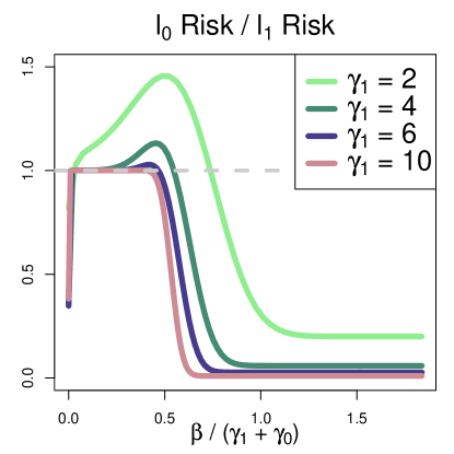
Because of the additivity of risk functions, (see appendix equations (LABEL:eqn:l0risk) and (LABEL:eqn:l1risk)), due to the orthogonality assumption, we focus on the individual behavior of $\beta_{i}$ for each single feature. Also the risk functions are symmetric on $\beta$, so only the cases of $\beta_{i}\geq 0$ will be displayed. Figure 2 illustrates that given $\gamma_{1}$, we can pick a $\gamma_{0}$, s.t. the risk ratio is below 1 for most $\beta$ except around $(\gamma_{0}+\gamma_{1})/2$, yet this ratio does not exceed one by more than a small factor, even for the worst case.

Figure 2: For each $\gamma_{1}$, we let $\gamma_{0}=\gamma_{1}+4\log(\gamma_{1})/\gamma_{1}$. This choice of $\gamma_{0}$ makes the risk ratios small at $\beta\approx 0$ and $\beta\geq\gamma_{0}$, only inflated around $\beta/(\gamma_{0}+\gamma_{1})=1/2$, albeit very little especially when $\gamma_{1}$ is large enough.

The intuition as to why $l_{0}$ fares better than $l_{1}$ in the risk ratio results is that $l_{1}$ must make a “devil’s choice” between shrinking the coefficients too much or putting in too many spurious features. $l_{0}$ penalized regression avoids this problem.

2.2 $l_{1}$ shrinks coefficients too much

Figure 3: Left: The $l_{0}$ estimate keeps the least squares value after the cutting point, but the $l_{1}$ estimate always shrinks the least squares estimate by a fixed amount. Middle: the model we simulate has only one true feature with true $\beta=1$ and a thousand spurious features. We compute the average Lasso estimate of $\beta$ for a fixed number of features included in the model (as an index of the $l_{1}$ penalty) from several different trials. $\bar{\hat{\beta}}_{l_{1}}$ is always shrunk by at least 20% in this experiment. Right: The Cauchy density has heavier tails than the Laplacian density does. Thus, a Laplacian prior tends to shrink large values of $\beta$’s.

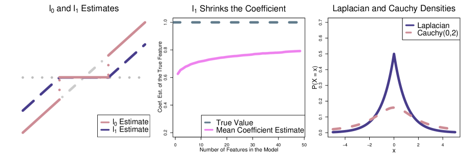
From a frequentist’s point of view, the $l_{1}$ estimator (2.1) shrinks the coefficients and thus is biased (Figure 3). In practice, $\hat{\beta}_{l_{1}}$ can be substantially shrunk towards zero when the system is sparse, as shown in the middle panel of Figure 3.

From a Bayesian’s perspective, the $l_{1}$ penalty is equivalent to putting a Laplacian prior on $\beta$ (Tib96; Efron+04), while the $l_{0}$ penalty can be approximated by Cauchy priors (JohnS05; FosterS05). The right panel of Figure 3 shows that the Cauchy distribution has a much heavier tail than the Laplacian distribution does. This implies that when the true $\beta$ is far away from 0, the $l_{1}$ penalty will substantially shrink the estimate toward zero.

The bias caused by the shrinkage increases the predictive risk proportionally to the squared amount of the shrinkage. The sparser the problem is, the greater the shrinkage is, thus the larger the risk is. These results show that in theory the $l_{0}$ estimate has a lower risk and provides a more accurate solution. Empirically, stepwise regression performs well in large data sets, where a sparse solution is particularly preferred (GeorgeF00; FosterS04; Zhou+06).

2.3 Simulations for Risk Ratio/flaws with l1

backgroundcolor=blue!20!white,inline, bordercolor=red]should mix some of the 1.2 and 1.3

2.3.1 $l_{1}$ optimization using an $l_{0}$ criterion

We can make use of the LARS algorithm to generate a set of candidate solutions and then use the $l_{0}$ criterion to find the best of the solutions along the regularization path. We evaluated this method as follows. We simulated $\mathbf{y}$ from a thousand features, only 4 of which have nonzero contributions, plus a random noise distributed as $N(0,1)$. Both the training set and the test set have size $n=100$. We apply the Lasso algorithm implemented by LARS on this synthetic data set. For each step on the regularization path, this algorithm selects a subset $\mathcal{C}\subset\{1,\ldots,1000\}$ of features that are included in the model. We then adopt a modified RIC criterion suggested in GeorgeF00:

$$\|\mathbf{y}-\mathbf{X}_{\mathcal{C}}\hat{\boldsymbol{\beta}}_{\mathcal{C}}\|_{2}^{2}+\sum_{q=1}^{|\mathcal{C}|}2\log(p/q)\sigma^{2}$$ (3)

to find an optimal $\mathcal{C}$. The crucial part here is that the coefficient estimate $\hat{\boldsymbol{\beta}}_{\mathcal{C}}$ being used in (3) is the least squares estimate of the true $\boldsymbol{\beta}$ obtained by fitting $\mathbf{y}$ on $\mathbf{X}_{\mathcal{C}}=(\mathbf{x}_{j})_{j\in\mathcal{C}}$, and not the Lasso estimate $\hat{\boldsymbol{\beta}}_{l_{1}}$ provided by the algorithm. We also use this least squares estimate in out-of-sample calculations.

Figure 4: $l_{0}$ penalties help finding the best model (independent predictors case). $\mathbf{y}$ is simulated from one thousand features, only four of which have nonzero contributions, plus an $N(0,1)$ error. Both the training set and the test set have sizes $n=100$. Each step in the LARS algorithm gives a set of features with nonzero coefficient estimates. We compute the least squares (LS) estimates on this subset and the modified RIC criterion (3) on the training set. We also compare the out-of-sample root mean squared errors using the LS estimates and the Lasso estimates on this LARS path. The features are independently generated. The model that minimizes the $l_{0}$ penalized error has exactly four variables in it. It also outperforms any of the $l_{1}$ models out-of-sample on this data set.

Figure 5: $l_{0}$ penalties help finding the best model (correlated predictors case). The setup is exactly the same as in Figure 4 except that each pair of features has a correlation $\rho=0.64$. In this case, the optimal model under the modified RIC criterion has a slightly better RMSE than the best $l_{1}$ model. The Lasso out-of-sample RMSE is typically minimized when the model has included more than 50 features.

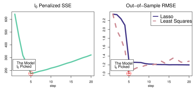
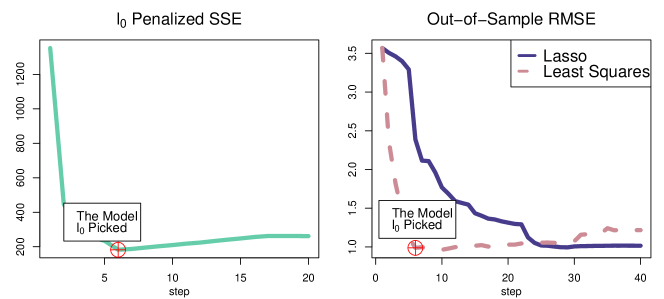
We compare two cases: the $\mathbf{x}_{j}$’s are generated independently of each other, meaning that $X^{\prime}X$ is diagonal, and the $\mathbf{x}_{j}$’s are generated with a pairwise correlation $\rho=0.64$. As shown in Figure 4, in the independent feature case, the model picked by the modified RIC criterion always outperforms any Lasso model on the test set. In the case with correlated predictors (Figure 5), there is little difference between the out-of-sample accuracies of the $l_{0}$-picked model and the best Lasso model in this case, but Lasso adds around 50 more spurious variables.

Thus, by combining the computational efficiency of an $l_{1}$ algorithm and the sparsity guaranteed by the $l_{0}$ penalization, we can easily select an accurate model without cross validation.

2.3.2 $l_{0}$ and NP-hardness

The $l_{0}$ problem is NP-hard and hence, at least in theory, intractable. (In practice, of course, people often use approximate solutions to problems that in the worst case can be NP-hard.) One of the attractions of $l_{1}$-regularization is that it is convex, hence solvable in polynomial time. In this section, we compare how the two approaches fare on a known NP-hard regression problem. We start with a simple constructive proof that the risk ratio for $l_{1}$ to $l_{0}$ can be arbitrarily bad. Construct data as follows. Pick a large number of independent features $z_{j}$. Construct new features $x_{1}=z_{1}+\epsilon z_{2}$ and $x_{2}=z_{1}-\epsilon z_{2}$ and. Let $y=(z_{1}+z_{2})/2$ plus noise. Then the correct model is $y=x_{2}/\epsilon$. Include the rest of the features $z_{j},j>2$ as spurious features.

In Nata95 the known NP hard problem of “the exact cover of 3-sets” was reduced to the best subset selection problem as below: $\mathbf{y}=\mathbf{1}_{n}$, $X$ is an $n\times p$ binary matrix with each column having three nonzero elements: $\|\mathbf{x}_{i}\|_{0}=3$, $\boldsymbol{\beta}$ is a $p\times 1$ vector, $\varepsilon>0$ and we want to solve r’c’l min_β ∥β∥_0, & s.t. ∥ y- Xβ∥_2¡ε. Note that if there is a solution to this problem, the number of features being chosen should be $n/3$.

We then ask which method comes closer to solving this problem: a greedy approximation to the $l_{0}$ problem or an exact solution to the $l_{1}$ problem. To this end, we applied Lasso and forward stepwise regression on various $n$’s. For small $n$’s, we took full collections of the three subsets, i.e., $p$ equals $n$ choose 3; for larger $n$’s, we took $p=10\cdot n$. Table 1 and 2 list the number of subsets included in the model. Forward stepwise regression always finds fewer subsets, and hence a better solution, than Lasso.

Method	$n=9$	$n=12$	$n=15$	$n=18$	$n=21$	$n=24$	$n=27$	$n=30$
Lasso	6	10	11	17	19	21	22	29
Stepwise	3	4	5	6	7	8	9	10

Table 1: The number of subsets chosen by Lasso and by forward stepwise regression with $\varepsilon=1/4$. All 3-subsets were considered, i.e., $p=\binom{n}{3}$. Forward stepwise regression always has the fewest possible number of subsets, namely, $n/3$.

Method	$n=99$	$n=240$	$n=540$	$n=990$	$n=1500$
Lasso	93	219	504	812	1372
	($2\times 10^{-23}$)	($9\times 10^{-23}$)	($9\times 10^{-15}$)	($6\times 10^{-20}$)	($2\times 10^{-20}$)
Stepwise	40	96	223	364	595
	($1\times 10^{-28}$)	($6\times 10^{-27}$)	($3\times 10^{-26}$)	($6\times 10^{-25}$)	($1\times 10^{-25}$)

Table 2: The number of subsets chosen by Lasso and by forward stepwise regression with $\varepsilon=1/4$. $p=10\cdot n$ 3-subsets were randomly chosen to be the predictors. Forward stepwise regression always chooses a sparser solution in the sense that it chooses fewer number of subsets. Numbers in parentheses are the sum of squared errors when the algorithms terminated.

All of our experiments on both synthetic and real data sets show that greedy search algorithms, such as stepwise regression, aimed at minimizing $l_{0}$-regularized error provide sparser results. This is because $l_{0}$ penalizes the sparsity directly, while $l_{1}$ does not. It is easy to construct an example where $l_{1}$ will pick a solution with a smaller $l_{1}$ norm but with a less sparse solution (CanWB07).

3 Conclusion

In many statistical contexts, the $l_{0}$ regularization criterion is superior to that of $l_{1}$ regularization; $l_{0}$ generally provides a more accurate solution and controls the false discovery rate better. $l_{1}$ can give arbitrarily worse predictive accuracy than $l_{0}$, since $l_{1}$ regularization tends to shrink coefficients too much to include many spurious features. Computationally, $l_{1}$ appears to be more attractive; convex programming makes the computation feasible and efficient. In practice, however, approximate solutions to the $l_{0}$ problem are often better than than exact solutions to the $l_{1}$ problem. The best properties of the two methods can be combined. Superior results were obtained by using convex optimization of the $l_{1}$ problem to generate a set of candidate models (the regularization path generated by LARS), and then selecting the best model by minimizing the $l_{0}$-penalized training error.

Appendix A Risk Ratio Proofs

We will drop the $\gamma$’s when the situation is clear, and denote $\hat{\beta}_{l_{0}}(\gamma_{0})$ as $\hat{\beta}_{l_{0}}$ and $\hat{\beta}_{l_{1}}(\gamma_{1})$ as $\hat{\beta}_{l_{1}}$ for simplicity.

Without loss of generality, we assume $\mathbf{X}^{\prime}\mathbf{X}=I$ and $\sigma=1$. The $l_{0}$ risk can be written as

rCl R(β,^β_l_0) & = E_β ∥Xβ-X^β∥^2 = E_β ∑