X-ray Polarization from High Mass X-ray Binaries

Abstract

X-ray astronomy allows study of objects which may be associated with compact objects, i.e. neutron stars or black holes, and also may contain strong magnetic fields. Such objects are categorically non-spherical, and likely non-circular when projected on the sky. Polarization allows study of such geometric effects, and X-ray polarimetry is likely to become feasible for a significant number of sources in the future. Potential targets for future X-ray polarization observations are the high-mass X-ray binaries (HMXBs), which consist of a compact object in orbit with an early type star. In this paper we show that X-ray polarization from HMXBs has a distinct signature which depends on the source inclination and orbital phase. The presence of the X-ray source displaced from the star creates linear polarization even if the primary wind is spherically symmetric whenever the system is viewed away from conjunction. Direct X-rays dilute this polarization whenever the X-ray source is not eclipsed; at mid-eclipse the net polarization is expected to be small or zero if the wind is circularly symmetric around the line of centers. Resonance line scattering increases the scattering fraction, often by large factors, over the energy band spanned by resonance lines. Real winds are not expected to be spherically symmetric, or circularly symmetric around the line of centers, owing to the combined effects of the compact object gravity and ionization on the wind hydrodynamics. A sample calculation shows that this creates polarization fractions ranging up to tens of percent at mid-eclipse.

1. Introduction

High mass X-ray binaries (HMXBs) are among the brightest X-ray sources in the sky. They consist of an accreting compact object (a neutron star or black hole) in orbit with an early type star (O or B star). They represent an important stage in the evolution of binary stars with early-type components, and they dominate the X-ray output of galaxies with young stellar populations. HMXBs emit X-rays via accretion onto the compact object by gas from the strong wind from the companion star, or from Roche lobe overflow. The X-rays interact with the accretion flow and stellar wind, producing observable signatures in timing and spectra. This provides a means to study the hot star wind and the accretion flow and the interaction of X-rays with these structures. One consequence of this interaction is the production of polarized X-rays via scattering. Polarization provides unique information into the geometry of the stars, wind and scattering region. In this paper, we explore the polarization signatures associated with this interaction.

There are $\simeq$10 HMXB sources with properties of their stellar winds and binary orbit which are well enough determined for quantitative modeling of the interaction of the accretion flow with X-rays (Kaper, 1998). The number of known HMXBs is many times greater when sources with less well constrained properties are included (Liu et al., 2006; Walter et al., 2015); these include sources discovered by INTEGRAL which are seen primarily at hard X-ray energies owing to obscuration, and transient sources which are detected primarily via long time-baseline monitoring. The most thoroughly studied systems include the objects Cyg X-1, Vela X-1, and Cen X-3. The majority of HMXBs contain pulsating neutron stars. If so, orbital eclipses, X-ray pulse timing and primary radial velocities (van der Meer et al., 2007) provides strong constraints on the orbital separations and masses. Simple estimates suggest that the accretion rate onto the compact object can be provided by the wind from the companion star in fewer than half the sources, while Roche lobe overflow is required in the remainder (Conti, 1978; White, 1985; Kaper, 1998). Though they are outnumbered by low mass X-ray binaries in our galaxy, these sources dominate the X-ray output from galaxies with larger star formation rates (Fabbiano, 2006). Their mass transfer can be very rapid; in a system in which the primary has a radiative envelope and fills its Roche lobe, the primary radius will shrink as a consequence of mass transfer, but if the mass transfer is conservative the Roche lobe will shrink more rapidly, potentially leading to a common envelope phase. If the primary is an evolved star with a convective envelope this outcome is more probable (Taam & Sandquist, 2000). Common envelope evolution when the primary is an evolved star is likely to lead to ejection of much of the envelope of the primary, leaving a binary consisting of a neutron star and the core of the primary. Whether due to nuclear evolution or to unstable mass transfer, their evolutionary lifetimes must be short ($\leq 10^{5}$ yrs).

The wind from the companion absorbs and scatters the X-rays from the accreting compact object in HMXBs, and the column densities traversed by the X-rays range from $\sim 10^{21}-10^{24}$cm^-2. The X-ray source luminosities range from $\sim 10^{35}-10^{38}$ erg s^-1. In sources where the X-ray source is luminous and the wind is weak, the wind is ionized throughout most of the region between the two stars. In systems with more massive winds and weaker X-ray sources X-ray-ionization effects are a perturbation on the wind properties. Key questions about HMXBs include the nature of the compact object: its mass, variability and intrinsic radiation pattern. Also of interest are the properties of the companion star wind and its uniformity in density and temperature. The X-ray source can provide a probe for the study of wind regions which are only weakly affected by ionization or the gravity of the compact object.

Many of the X-ray properties of HMXBs are affected by the stellar wind and accretion flow. This includes the variability around the orbit, which shows gradual eclipse transitions due to photoelectric absorption in the wind (Clark et al., 1988), enhanced absorption at late orbital phases due to a wake or stream trailing the compact object (Kallman & McCray, 1982; Watanabe et al., 2006). The wind and accretion flow also provide torque to the compact object and regulate its spin or angular momentum. The structure of the wind and accretion flow is uncertain; winds from comparable single O or B stars have radiatively driven winds (Lamers & Cassinelli, 1999) which are affected by instabilities (Owocki et al., 1988), shocks (Lucy & White, 1980) and clumping (Cohen et al., 2006); observations provide the most reliable means for understanding these processes, via fitting of parameterized models. In addition, the compact object affects the gas flow, via its gravity and also X-ray heating and ionization.

The next new astrophysical window will be the advent of measurements of X-ray polarization (Jahoda et al., 2014; Weisskopf et al., 2013). Among other things, polarization allows for potentially sensitive tests of the geometry of astrophysical sources, on scales which are far too small to be imaged directly. There is only one source in the sky whose X-ray polarization is known, the Crab nebula (Weisskopf et al., 1978). Owing to visibility constraints, it is likely that the first astronomical X-ray polarimetry observations will be of objects which have never before been observed with this technique. This motivates thorough and accurate modeling of the polarization properties of the brightest and (otherwise) best understood X-ray sources, for use as calibrators and test sources for X-ray polarimetry. HMXBs are among the sources best suited for this. Their orbital elements are relatively well understood and their orbital variability provides a predictably changing view with respect to an important source of polarization: the strong stellar wind from the companion star. X-ray polarimetry provides a means to probe the structure and the physical processes occuring in and near compact objects, on length scales too small to be imaged directly. In spite of scanty astrophysical detections so far (Weisskopf et al., 1978) it is of interest to consider the possible signals and diagnostic use of X-ray polarization in known classes of cosmic sources, as it is likely that instruments with improved sensitivity will become available eventually.

Polarization properties of HMXBs have been discussed previously in the context of scattering of optical and UV from the primary star (Brown & McLean, 1977; Brown et al., 1978; Rudy & Kemp, 1978). These authors predicted that the linear polarization has a characteristic variability around the binary orbit, associated with scattering in the stellar envelope which is distorted by the gravity of the compact object. This variability can be used as a diagnostic of the shape of the star, and also of the inclination of the binary orbit. These effects are observed at the predicted level in some systems; their absence in other cases suggests that the optical light may be affected by contributions from structures whose shape is not symmetric around the line of centers. Related work has been carried out by Al-Malki et al. (1999); Ignace et al. (2009); Nofi & Wiktorowicz (2014). Useful formalism for the calculation of polarization has been provided by Matt et al. (1996). The polarization properties of the accretion columns in X-ray pulsars have been calculated by (Meszaros et al., 1988). Predictions of X-ray polarization by the large scale structures in binaries has been carried out for distorted stars (Angel, 1969); for Compton scattering within the accretion column of magnetic cataclysmic variables (McNamara et al., 2008), following up on pioneering work by Matt (2004).

X-rays have an important advantage over optical light which is that the source is almost certainly compact compared with the size of the binary system. That is, we expect X-rays to be emitted from a region smaller than the Alfven shell, defined as the distance from the compact object where the pressure due to a dipole magnetic field balances the ram pressure of accretion. For fields $\sim 10^{12}$ Gauss this region has a size $\sim 10^{8}$ cm (Lamb et al., 1973). Far outside this region the influence of the field on the dynamics is negligible. The Alfven shell size can be compared with the primary star radius and orbital separation which are $\sim 10^{12}$ cm. This disparity in sizes greatly simplifies the geometrical considerations associated with the use of X-ray polarization since the X-ray source is effectively a point source when considering the effect of the scattering by the stellar wind. Calculating the polarization from these structures is straightforward, given certain simplifying assumptions, though it is important to take into account the effects of atomic absorption and resonance line scattering, which in turn depends on the gas dynamics, along with electron scattering.

The polarization properties of HMXBs will be affected by the intrinsic polarization of the compact X-ray source, and by the polarization imprinted by the stellar wind and accretion flow. These can be distinguished by their differing variability behavior: the compact source generally varies on a pulsation timescale for sources containing a pulsar, which is $\sim$ seconds – minutes. The very few sources which contain black holes also have their strongest intrinsic variability on comparably short timescales. Wind variability, on the other hand, is associated with the orbital timescale ($\sim$ days) or possibly on the wind flow timescale which is $\geq$hours. In some HMXBs the X-ray source is luminous enough to ionize the wind almost completely, so the light observed during and near eclipse, and its polarization, is dominated by electron scattering.

In this paper we present a general discussion of the behavior of X-ray polarization from HMXBs as a function of the parameters of the system and the viewing position. We present calculations of the polarization signature for various simple analytic models for the wind density and ionization structure, and discuss the dependence of these on parameters: wind optical depth, inclination, and viewing direction or orbital phase. We also explore the effects of wind hydrodynamics, i.e. departures from spherical symmetry due to the effects of the X-ray source gravity and heating. We utilize sample three-dimensional dynamical models. We take the intrinsic polarization of the compact object as unpolarized and explore the combined effects of geometry and scattering physics on the predicted linear polarization in the 0.1 - 10 keV X-ray band.

In section 2 we present numerical calculations for spherical winds using only electron scattering. The effects of resonance line scattering are discussed in section 3. In section 5 we present models which include photoelectric absorption and an ensemble of resonance scatterers. In section 6 we present models utilizing three-dimensional hydrodynamic models for the wind density and velocity field. We use these to derive approximate predictions for the polarization levels expected for several well known systems in section 7. The Appendix presents simple analytic estimates of the polarization for idealized HMXB conditions; many of these mirror earlier results. The computational techniques and level of detail we employ are similar to those of our previous work (Dorodnitsyn & Kallman, 2010) on the polarization from warm absorbers in Syefert galaxies.

2. Spherical Winds

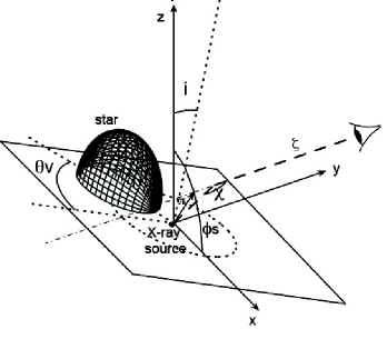
The basic geometry of an HMXB is illustrated in figure 1. This shows a schematic of an HMXB with a typical orbital separation and a sample X-ray ionized zone. It also shows the geometry we use when calculating the polarization: the X-ray source is at the origin and the primary orbits in a plane inclined by an angle $i$ to the line of sight. The orbital phase is described by the angle $\Theta_{V}$ relative to the line of centers. The system is viewed along the y axis.

In this section we will consider the simple case in which the wind density is spherically symmetric about the primary star, and the only interaction between the X-rays and the wind is electron scattering. If so, the scattering phase function follows the Rayleigh form (Chandrasekhar, 1960). The scattered emissivity at each point depends only on the local gas density and on the flux from the X-ray source. We assume the X-ray source radiates isotropically with a constant total luminosity $L_{0}$ and is unpolarized.

We calculate the polarization signatures in the form of the three Stokes parameters for linearly polarized light using the formal solution to the equation of transfer (Mihalas, 1978).

$$\left\{\begin{matrix}L(\varepsilon)\\ Q(\varepsilon)\\ U(\varepsilon)\end{matrix}\right\}=\int dV\kappa(\varepsilon,{\bf r})S(\varepsilon,{\bf r})e^{-\tau(\varepsilon,{\bf r})}\left\{\begin{matrix}1+\cos^{2}\chi\\ \sin^{2}\chi\cos(2\gamma)\\ \sin^{2}\chi\sin(2\gamma)\end{matrix}\right\}$$ (1)

where $\varepsilon$ is the photon energy, $S(\varepsilon,{\bf r})$, is the source function, $\kappa(\varepsilon,{\bf r})$ is the opacity, $\tau(\varepsilon,{\bf r})=\int{\kappa(\varepsilon,{\bf r})d\zeta}$ is the optical depth from a point ${\bf r}$ to a distant viewer, $\chi$ is the scattering angle and $\gamma$ is the angle between the scattering plane and a reference direction on the sky. Here and in what follows we describe the Stokes parameters in terms of the luminosity seen by a distant observer, i.e. the total energy (in ergs s^-1 sr^-1) radiated by the system in that direction. Equation 1 defines the scattered luminosity, $L$ (polarized plus unpolarized); observations are also affected by an unscattered component, $L_{u}(\varepsilon)=L_{0}(\varepsilon)e^{-\tau(\varepsilon,{\bf r_{x}})}$ where ${\bf r_{x}}$ is the position of the X-ray source. For the purpose of evaluating these quantities we adopt a cylindrical coordinate system with the X-ray source at the origin and the viewing direction along the $\hat{\bf y}$ axis. The angle $\gamma$ corresponds to the azimuthal angle on the plane of the sky and is measured relative to a line which is the intersection between the orbital plane and the plane of the sky. In the case of pure electron scattering the source function is $S=L_{0}/(4\pi r_{x}^{2})$ where $r_{x}$ is the distance from the X-ray source and the opacity is $\kappa(\varepsilon,{\bf r})=n({\bf r})\sigma_{Th}$.

Some useful results are presented in the Appendix. The fractional polarization relevant to observation is $P=\sqrt{(Q^{2}+U^{2})}/(L+L_{u})$. This quantity is zero when the system is viewed at inclination $i=\pi/2$ and at either conjunction, i.e. orbital phase 0.5 or 1, $\Theta_{V}=0$ or $\pi$. The polarization at $i=\pi/2$ is a maximum at quadrature, phase 0.25 or 0.75. We can also define the polarization of the scattered radiation only, i.e. $P_{s}=\sqrt{(Q^{2}+U^{2})}/L$, and the value of this quantity at quadrature and $i=\pi/2$ depends only on the orbital separation and on the distribution of gas density in the wind. The value of $P$ is less than the value of $P_{s}$ by a factor proportional to the Thomson depth whenever the X-ray source is not eclipsed. At $i=0$, i.e. when the system is viewed face-on, the polarization rotates with orbital phase at a rate twice the orbital rotation rate.

As an illustration of these results, we calculate the polarization produced by a single-scattering calculation by numerically evaluating equation 1. The wind velocity is assumed to be radial relative to the star with a speed given by $v(r)=v_{0}+(v_{\infty}-v_{0})(1-r_{*}/r)$ where the terminal velocity is $v_{\infty}$=1000 km s^-1 and $v_{0}$=100 km s^-1, and $r_{*}=10^{12}$ cm. The wind mass loss rate is $\dot{M}_{wind}=10^{-8}M_{\odot}{\rm yr}^{-1}$. The orbital separation is $a=1.5r_{\*}$.

In the remainder of this paper we discuss quantitative calculations of polarization produced by wind scattering. These include calculations based on both the very simple spherical wind with parameters given in the previous paragraph and also on hydrodynamic calculations of the wind density structure which make no assumptions about spherical symmetry. In the former case, it is illuminating to estimate the accretion rate onto the compact object if the accretion is supplied solely by the wind. This can be done using simple estimates based on Bondi & Hoyle (1944) and Davidson & Ostriker (1973), i.e. $\dot{M}_{acc}=\pi R_{acc}^{2}n_{x}v_{x}m_{H}$ where the accretion radius is $R_{x}=2GM/v_{x}$, $M$ is the mass of the compact object and $v_{x}$ is the speed of the wind at the X-ray source. This corresponds to $\dot{M}_{acc}/\dot{M}_{wind}=1.8\times 10^{-4}(M/M_{\odot})^{2}v_{x8}^{-4}a_{12}^{-2}$ where $v_{x8}=v_{x}/(1000{\rm kms}^{-1})$, $a_{12}=a/(10^{12}{\rm cm})$ or an X-ray luminosity $L_{x}\simeq 1.8\times 10^{35}{\rm ergs}^{-1}$ using the parameters given in the previous paragraph and assuming an efficiency of converting accreted mass into energy of 0.1. This luminosity is less than the time averaged luminosities of most HMXBs by factors $\sim$5 – 100, which likely reflects the fact that wind mass loss rates may be greater, additional mass can be supplied by Roche lobe overflow, and the wind and accretion flow dynamics can be enhanced by the influence of the compact object gravity and ionization. The results in what follows, those which are based on the simple spherical wind approximation, must interpreted subject to this caveat.

An additional caveat which applies to essentially all of the results presented in this paper is the assumption of single scattering. The validity of this assumption depends on the wind optical depth from the X-ray source; multiple scattering is important when this quantity approaches or exceeds unity. For parameters similar to those discussed so far, this quantity for a distant observer corresponds to $\tau_{Th}\sim n_{x}a\simeq 2\times 10^{-4}\dot{M}_{8}a_{12}^{-1}v_{x8}^{-1}$, where $\dot{M}_{8}=\dot{M}/(10^{-8}M_{\odot}{\rm yr}^{-1})$. Comparing this expression with the accretion luminosity estimate given above implies that multiple scattering can be important when the accretion luminosity exceeds $\sim 10^{38}{\rm ergs}^{-1}$ for a 1 $M_{\odot}$ compact object. The likely effect of multiple scattering is to produce smaller net polarization than for single scattering, since the second and subsequent scatterings have a wider range of scattering angles and planes than for single scattering. If the depth is moderate, i.e. $\leq$ 10, there will still be a significant fraction of photons which reach the observer after a single scattering. If so the net polarization will likely be less than predicted here, by factors of order unity, and our results should be modified to include multiple scattering effects for such sources.

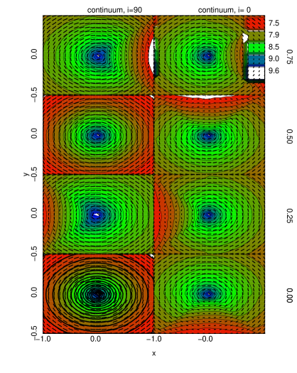
Maps of polarization projected against the sky are shown in figure 2. This shows contours of constant intensity as solid colors separated by solid black curves, along with lines corresponding to polarization vectors, which appear as dashed curves. These are plotted vs position in units of $10^{12}$ cm. These illustrate many of the results presented in the Appendix: At high inclination, $i=\pi/2$, and at orbital phase angles 0 and $\pi$ (orbital phases 0 and 0.5) polarization vectors are perfectly circumferential, contours of constant intensity are also circular and the net polarization is zero. At orbital phase angles $\pi/2$ and $3\pi/2$ (orbital phases 0.25 and 0.75) the net polarization is maximum. At inclination $i=0$ the star always influences the polarization, so that the net polarization fraction is constant, but the position rotates with the orbit.

Figure 1.— Schematic of high mass X-ray binary (HMXB) as viewed from above the orbital plane, showing typical orbital separation and companion star size. Coordinates are labeled according to their use in the Appendix.

Figure 2.— Map of intensity and polarization vectors projected on the sky for four orbital phases and two inclinations. Colors correspond to scattered intensity according to the color bar, in which the labeled quantities correspond to log₁₀ of the specific intensity. Short black lines correspond to polarization vectors. Spherically symmetric wind is assumed.

More insight comes from the Stokes quantities as a function of the orbital phase. These are shown in figure 3 for inclinations $i=0$ and $i=\pi/2$. U is green while Q is shown in red; solid is $i=\pi/2$ and dashed is $i=0$. This further illustrates the results from the previous figure: at $i=0$ the polarization oscillates between Q and U along orbital phase, and the vector sum is constant. At $i=\pi/2$ U is always small (in this convention) and Q is a maximum at phase angles $\pi/2$ and $3\pi/2$. Another way of displaying the same thing is shown in figure 4, which shows U plotted vs Q, for $i=0$ in green, and $i=\pi/2$ in red. This shows that the trajectory of U vs. Q is circular at $i=0$ and becomes linear at $i=\pi/2$. As shown by Brown et al. (1978), this trajectory is an ellipse for intermediate inclinations, and the cases in figure 3 are the extremes of eccentricity. This has been suggested as a means for measuring inclination (Rudy & Kemp, 1978).

Figure 3.— Stokes parameters for spherical wind, Q (red ) and U (green) vs. phase for inclinations $i=0$ (dashed) and $i=\pi/2$ (solid). The total intensity I is shown as dashed black for $i=0$. At $i=0$ the polarization oscillates between Q and U along orbital phase, and the vector sum is constant. At $i=\pi/2$ U is always small (in this convention) and Q is a maximum at phase angles $\pi/2$ and $3\pi/2$.

Figure 4.— Stokes parameters for spherical wind, Q vs U $i=0$ (green) and $i=\pi/2$ (red). This again illustrates the circular path of the net polarization direction with orbital phase at $i=0$ and the constancy of the direction at $i=\pi/2$.

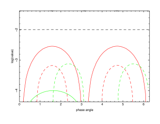
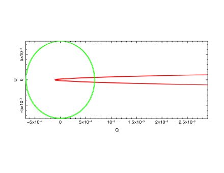
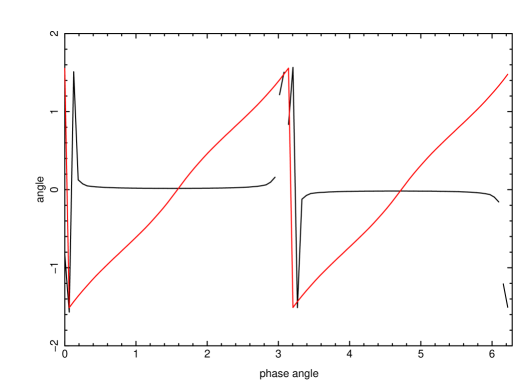
Figure 5 shows the scattered polarization fraction vs. orbital phase, i.e. $P_{s}=\sqrt{(Q^{2}+U^{2})}/L$. This shows that the maximum polarization fraction is $\simeq$10$\%$ for the parameters chosen here, when the polarized component is compared with the total scattered component. This is comparable to the result in the Appendix, calculated for a thin shell at the star rather than for an extended wind. We emphasize that this value depends primarily on geometric quantities: the extent of the wind, and orbital separation relative to the stellar radius. It does not depend on the wind density or column density since it is a comparison of scattered quantities. The difference between $i=0$ and $i=\pi/2$ is clearly apparent: the former produces approximately constant polarization fraction and the latter oscillates between 0 and a value comparable to the $i=\pi/2$ value. Figure 6 shows the polarization fraction measured relative to the total radiation, scattered plus direct, i.e. i.e. $P=\sqrt{(Q^{2}+U^{2})}/(L+L_{u})$. This illustrates the diluting effect of the direct radiation for this model, which has $\tau_{Th}\simeq 0.25$. Maximum linear polarization at $i=\pi/2$occurs just following the eclipse transition, where the departures from circular symmetry on the sky are not negligible, and where the direct radiation is blocked by the primary star. At mid-eclipse the polarization at $i=\pi/2$ is zero due to symmetry. Figure 7 shows the polarization angles from the same set of models. The angle sweeps through 180 degrees twice per orbital period for $i=0$, while the angle is constant (though undefined near conjunctions) for $i=\pi/2$.

Figure 5.— Polarization fraction of scattered radiation i.e. $P_{s}=\sqrt{(Q^{2}+U^{2})}/L$ for spherical wind, $i=0$ (red) and $i=\pi/2$ (black).

Figure 6.— Polarization fraction relative to total radiation, scattered plus direct, for spherical wind, $i=0$ (red) and $i=\pi/2$ (black).

Figure 7.— Polarization angle for spherical wind, $i=0$ (red) and $i=\pi/2$ (black).

3. Resonance Line Scattering: Single Line

The models discussed in section 2 include solely electron scattering; they do not include resonant scattering in bound-bound transitions. This process (when associated with UV and optical transitions) is the dominant driving mechanism for the winds from early type stars. Here we consider scattering in the X-ray band. In the absence of X-ray ionization, the ions which are most abundant in early-type star winds are in charge states from $\sim$1 – 5 times ionized, and do not have many strong X-ray resonance line transitions. Ionization by a compact X-ray source can produce ions of arbitrary charge state, depending on the X-ray flux and gas density, and so resonance scattering can affect the scattered X-ray intensity and polarization. The ionization structure in HMXB winds has been explored by Hatchett & McCray (1977) who showed that the surfaces of constant ionization in a spherical wind are either nested spheres surrounding the X-ray source, or else open surfaces enclosing the primary star. The ionization distribution depends on a parameter $q=\xi/\xi_{x}$ where $\xi_{x}=L_{x}/(n_{x}a^{2})$ where $L_{x}$ is the ionizing X-ray luminosity, $n_{x}$ is the gas density at the X-ray source and $a$ is the orbital separation. This is a particular example of the scaling of ionization in optically thin photoionized gas, which depends on the ionization parameter $\xi=L_{x}/(n(r)r_{x}^{2})$ (Tarter et al., 1969; Kallman & Bautista, 2001). The properties of resonance scattering as applied to X-ray polarization in HMXBs are dominated by the fact that, owing to the restricted regions where ionization is suitable, most lines can only have strong opacity over a fraction of the wind. The regions where this occurs most often resemble spherical shells surrounding the X-ray source.

Resonance scattering differs from electron scattering in its sensitivity to the velocity structure of the wind. At a given observed photon energy, scattering can occur only over a resonant surface with shape determined by the wind velocity law; in a spherical wind with monotonic velocity law these surfaces are open surfaces of revolution symmetric about the line of sight to the X-ray source.

Resonance scattering affects polarization by redistributing the polarization among the components of the Stokes vector according to the phase matrix which is a linear combination of the Rayleigh and isotropic phase matrices; coefficients of the matrix depend on the angular momentum quantum numbers of the initial and final states of the transition, $j$ (Lee et al., 1994). The matrices describing this process have been calculated by Hamilton (1947). In practice most of the strongest X-ray resonance lines have initial and final values $j_{lower}=1/2$ and $j_{upper}=3/2$, which correspond to the Rayleigh phase matrix, and we adopt this in our calculations. Similar assumptions were employed in Dorodnitsyn & Kallman (2010).

Polarization also depends on the scattering angle, and the resonance condition constrains the scattering geometry, thereby imposing a relation between the energy of the scattered photon and its polarization. Resonance scattering can have a cross section which is much greater than electron scattering, but only over the relatively narrow energy band spanned by the resonance line, including the effects of Doppler broadening associated with the wind motion. Within this band, the polarization can be greater than that produced by electron scattering, owing to the greater cross section, given suitable geometry.

In the remainder of this section we illustrate these effects by generalizing the single scattering spherical wind calculations to include resonance scattering. We consider a single resonance line, chosen to crudely resemble a line such as O VIII L$\alpha$. The parent ion is assumed to exist over a range of ionization parameter $1\leq{\rm log}(\xi)\leq 3$. We calculate the optical depth using the Sobolev expression (Castor, 1970):

$$\tau_{line}(\varepsilon,{\bf r})=\frac{\pi e^{2}}{mc}fn({\bf r})x_{ij}y_{j}\frac{\lambda r}{v(r)(1+\frac{z^{2}}{r^{2}}\left(\frac{d{\rm ln}v(r)}{d{\rm ln}r}-1\right)}$$ (2)

where $f$ is the oscillator strength, $n({\bf r})$ is the gas number density, $x_{ij}$ is the ion fraction, $y_{j}$ is the element abundance, $z$ is the position along the line of sight, and $\lambda$ is the line wavelength. For the source function we adopt the same expression used for electron scattering $S=L_{0}/(4\pi r_{x}^{2})$ since thermalization is unimportant and the size of the X-ray source is small compared with the other length scales of interest for HMXBs.

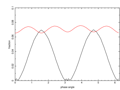
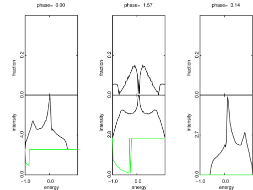
Results of our simple single line calculation are shown in figure 8. This shows the line profile as a function of orbital phase for a system viewed edge on ($i=\pi/2$). For each phase we display the luminosity, with the transmitted luminosity shown in black and the scattered luminosity shown in green (bottom panel) and polarization fraction (top panel). The polarization angle is not shown because there is no significant dependence on energy or orbital phase when the system is viewed at high inclination; the polarization is always perpendicular to the orbital plane. The horizontal axis is energy in units of the wind terminal velocity.

At phase 0 (superior conjunction of the X-ray source) the shape of the profile in luminosity is similar to P-Cygni profiles familiar from UV resonance lines in hot stars: the outflow produces blue-shifted absorption (shown as negative energy in these figures) of the continuum. This absorption is offset from the zero of energy owing to the fact that the continuum source in this case is the compact X-ray source, and the wind speed at the X-ray source is approximately half the terminal speed. In addition, the X-ray source creates an ionized region within which line scattering cannot occur. As a result, the absorption occurs in a relatively narrow region of energy near the energy corresponding to the wind terminal velocity. The scattered emission, on the other hand, is essentially symmetric in energy, since scattered emission comes from a region which is not necessarily along the line of sight to the X-ray source. Projection effects make the scattered emission appear at all energies $|\varepsilon|\leq\varepsilon_{0}v_{\infty}/c$ where $\varepsilon_{0}$ is the line rest energy. The scattered emission is unpolarized at phase 0 for the same reason as in the pure electron scattering case. At phase 0.25 (quadrature) the wind is viewed perpendicular to its velocity vector at the X-ray source, and therefore the absorption covers a large fraction of the energy spanned by the wind. The scattered emission is polarized up to $\sim$50$\%$; the degree of polarization is symmetric around the center of the line, owing to the fact that the wind velocity structure is symmetric around the line of centers. At phase 0.5 (inferior conjunction of the X-ray source) there is no transmitted flux (due to occultation by the star) and the emission is predominantly red-shifted owing to the location of the X-ray ionized zone in the receding part of the wind. In this case, even though the flux is all scattered, the polarization fraction is negligible owing to the circular symmetry of the scattering region of the wind as viewed in the plane of the sky.

Figure 8.— Spectrum, polarization fraction and angle in a resonance line vs. energy in units of the terminal velocity at orbital phase 0.25 for inclination $i=\pi/2$

4. Absorption Effects

The ionization balance in an HMXB wind is determined at each point by the X-ray flux and by the gas density. The X-ray flux in turn depends on the effects of geometrical dilution and on attenuation. In order to do so, we utilize results from xstar (Kallman & Bautista, 2001) at each point in the wind in order to determine the opacity. This is done along radial rays originating from the X-ray source, so that the opacity at each point is calculated using an ionization parameter which corresponds to the flux transmitted along the corresponding ray.

This single stream transfer treatment is similar to the transfer treatment used by xstar with one difference: xstar uses the local spectral energy distribution (SED) to calculation the ionization along a ray; here we use the same unattenuated SED everywhere for the ionization calculation (so we can use a stored table), but we calculate the ionization parameter self-consistently, i.e. by calculating the transmitted flux at each position and then using that value to calculate the ionization parameter. This simplification allows for more efficient computation without unduly sacrificing physical realism. This approximation will be least accurate when the column density is highest, i.e. $\geq 10^{23}$ cm^-2. In such regions, the ionization is expected to be low, owing to attenuation, and X-ray scattering will be relatively unimportant. Our approximation will tend to produce less attenuation at a given column density than a self-consistent calculation would.

5. Resonance Line Scattering: Ensemble of Lines

X-ray ionization creates an ensemble of resonance lines in an HMXB wind from the many trace elements such as C, N, O, Ne, Mg, Si, S, and Fe. At any point in the wind the ionization depends most sensitively on the ionization parameter, defined in the previous section. Figure 9 shows the distribution of ionization parameter produced in a wind with a density distribution which is spherically symmetric around the primary star, as discussed so far. We adopt a spherical wind with mass loss rate $10^{-5}M_{\odot}{\rm yr}^{-1}$, corresponding to a total wind column density of $3\times 10^{23}$ cm^-2, and an X-ray source luminosity of $10^{38}$ erg s^-1. Each spatial region with a distinct ionization parameter will have a different distribution of ion abundances, and hence a unique distribution of resonance line opacity. These can be calculated under the assumption of ionization equilibrium. Figure 10 show examples of the spectrum and the polarization fraction produced by such a distribution from the spherical wind shown in figure 9. Ionization and line opacities were calculated as a function of ionization parameter using the xstar code (Kallman & Bautista, 2001). These were binned into 1000 energy bins over energy from 0.1 eV to 10⁴ eV. Since the Doppler shifts associated with the wind speed is less than the energy bin size, we adopt an approximate form for the source function each resonance line:

$$S(\varepsilon,{\bf r})=\frac{L_{0}}{4\pi r_{x}^{2}}\frac{v_{\infty}-v_{0}}{\Delta\varepsilon c/\varepsilon}$$ (3)

where the quantity $(v_{\infty}-v_{0})/(\Delta\varepsilon c/\varepsilon)$ takes into account the fact that the line does not conver the entire energy bin. This treatment assumes that the line optical depths are not large, which is an adequate approximation for our situation. Depolarization effects at large Sobolev optical depths associated with multiple scatterings are not taken into account. These calculations serve to illustrate the magnitude of the polarization effects expected from resonance scattering in HMXBs. Simulations suitable for quantitatively diagnosing the wind or the X-ray source properties will require reexamination of these assumptions.

Results of spectra and polarization fractions are shown in figure 10. These demonstrate that the resonance lines cover a significant fraction of the X-ray energy band and that they can scatter a significant flux of X-rays, and create polarization fractions as high as 0.5, much greater than would be produced by electron scattering alone. A difference between resonance scattering and electron scattering is that resonance scattering in a given line occurs within a relatively narrow spatial region where the parent ion is most abundant. For X-ray lines, these are most likely to be approximately spherical surface surrounding the X-ray source. This region tends to produce a small polarization which is almost independent of the viewing angle. Thus resonance scattering produces weaker modulation of the polarization with orbital phase than does electron scattering.

It is also worth noting that the effects of scattering can be either polarizing or not polarizing, depending on the scattering angle. Also, lines which appear in absorption in the spectrum can have enhanced polarization in their troughs owing to the presence of scattered light in the residual intensity. In the spectrum shown in figure 10 the polarization in the absorption lines is generally lower than in the emission features, or in the adjacent continuum. This is due to the fact that the scattered light in the residual intensity is forward scattered, and so is not polarized because of the scattering angle.

Figure 9.— Distribution of ionization parameter in the orbital plane for a spherical wind with $\dot{M}_{wind}=10^{-5}M_{\odot}{\rm yr}^{-1}$ illuminated by a 10³⁸ erg s^-1 X-ray source. Contours are labeled with log$\xi$.

Figure 10.— Spectrum and polarization fraction vs energy for spherical wind in units log(E/keV) at orbital phase 0.25 for inclination $i=\pi/2$

6. Hydrodynamic Models

The stellar wind in HMXBs is not spherically symmetric. Physical processes which affect the wind and accretion flow in HMXBs include: the three-dimensional geometry of the flow (i.e. the flow both in and out of the orbital plane), rotational forces, the influence of gravity and radiation pressure from both stars in the binary, transport of the radiation from the stars into the flow and the reprocessed radiation out of the flow, X-ray heating and ionization, and departures from thermal equilibrium due to advection and adiabatic heating and cooling. The dynamics of X-ray heated winds have been discussed by Fransson & Fabian (1980), and Hatchett & McCray (1977), and multi-dimensional models have been calculated by Blondin et al. (1990); Blondin (1994); Mauche et al. (2008)

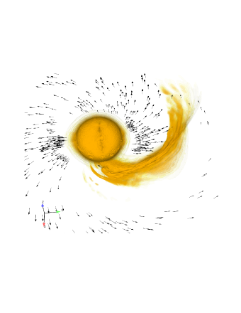
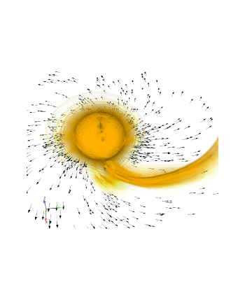
In this section we illustrate the effects of the wind hydrodynamics on the polarization. We use two sample wind hydrodynamic models calculated using a numerical model similar to that described in Blondin & Pope (2009) but extended to three dimensions. The hydrodynamic models are computed on one hemisphere of a spherical grid, assuming reflection symmetry about the orbital plane. A non-uniform grid of 448 (r) by 128 ($\theta$) by 512($\phi$) zones is used with highest resolution near the surface of the primary star and in the vicinity of the accreting neutron star. This model calculates the wind dynamics in three dimensions taking into account the radiative driving by the UV/optical radiation from the primary, and also the gravity of the star and the compact X-ray source. A fixed X-ray luminosity of 10³⁶ erg/s is used to calculate X-ray heating using the approximate formulae given in Blondin (1994) and the effects of X-ray ionization on the dynamics via changes in the UV radiation force multiplier. The two models have identical dimensions: primary radius 2.4 $\times 10^{12}$ cm and orbital separation 3.6 $\times 10^{12}$ cm. They differ in their mass loss rates, which are 4 $\times 10^{-7}M_{\odot}{\rm yr}^{-1}$ and 1.7 $\times 10^{-6}M_{\odot}{\rm yr}^{-1}$. The maximum wind speed in both models is approximately 1600 km s^-1. A plot showing the density contours and velocity vectors is shown in figure 11. This clearly shows the influence of the gravity of the compact object in creating a region of higher density and non-radial wind flow in the vicinity of the X-ray source.

The distorted stellar wind of the hydrodynamic models is illustrated with velocity vectors in the orbital plane and a series of transparent density isosurfaces. Right panel is the model with a higher mass loss rate (Mdot = 1.7e-6); left panel is a lower mass loss rate (Mdot = 4.0e-7). The lowest density isosurface corresponds to a density of 4e9 cm^-3 in both panels. Velocity vectors are not shown for values less than 800 km/s.

The high mass loss rate model has a denser spherical component of the wind, but a less pronounced accretion wake. The low mass loss rate model has a larger volume of wind moving at low velocity due to photoionization of the wind in the vicinity of the X-ray source. The result is a denser wind coming off the primary along the line of centers of the binary system and a larger, denser accretion wake that wraps more tightly around the primary star.

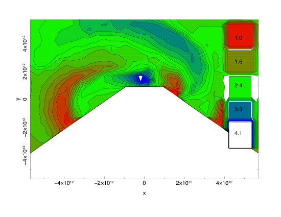
We apply the same calculation of X-ray scattering to the hydrodynamic wind as was done in section 3. We assume an X-ray source luminosity of $10^{36}$ erg s^-1 and a $\Gamma$=2 power law ionizing spectrum. The distribution of ionization parameter in the orbital plane is shown in figure 12. This shows a spiral structure, owing to a corresponding structure in the gas density.

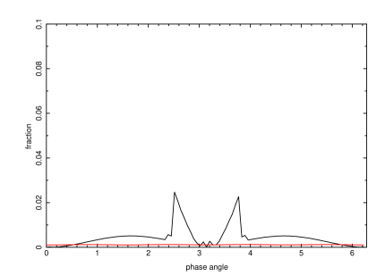
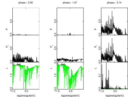
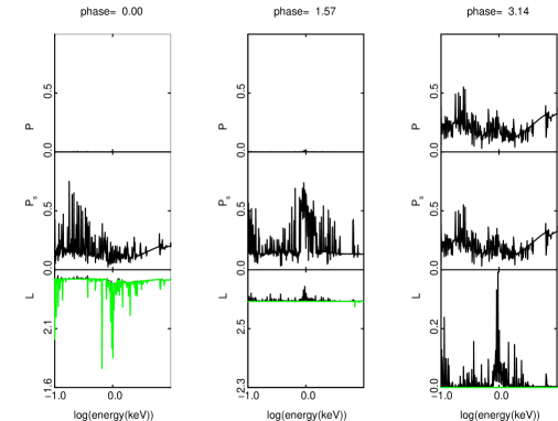
Figures 13 shows the spectra and polarization produced by the hydrodynamic wind model with $\dot{M}=4.0\times 10^{-7}M_{\odot}{\rm yr}^{-1}$ at orbital phases 0, 0.25 and 0.5. Comparison with figure 10 shows that the hydrodynamic model produces a spectrum which is similar to that from a smooth spherical wind. However, the degree of polarization is significantly greater, due to the departure from spherical symmetry created by the X-ray source. In particular, the spectrum during eclipse is greater, owing to the fact that the wake structure extends beyond the disk of the primary star during eclipse. The spherical wind produces fractional polarization averaged over the 0.1 – 10 keV energy band, of at most 10$\%$ during eclipse. The spherical wind produces polarization values which are much less than this at mid-eclipse. The hydrodynamic wind produces fractional polarization of approximately 21$\%$ at mid-eclipse.

Polarization calculations for hydrodynamic models have been carried out for the two mass loss rates shown in figure 11, and for several choices of ionizing X-ray luminosity. Note that the hydrodynamic models assume a fixed X-ray luminosity (used to calculate X-ray heating and ionization within the simulation) of 10³⁶ erg/s, independent of the X-ray luminosity used to calculate the spectrum and polarization. Moreover, the prescribed X-ray luminosity is not generally consistent with the mass accretion rate derived from the hydrodynamic simulation, and thus these models are not fully self-consistent. Nonetheless, they serve to illustrate the behavior of the polarization and its dependence on wind density and X-ray luminosity.

Values for polarization fractions during eclipse are shown in table 1. These are averages of the linear polarization over energy in the range from 0.1 – 10 keV. Polarization values reflect competing effects. For highly ionized gas, the wind is essentially transparent and the polarization is due to Thomson scattering. The polarization fraction is proportional to the Thomson depth (when small) and also to departures from circular symmetry of the scattering material in the plane of the sky. Partially ionized gas can produce larger polarization, owing to the greater cross section associated with resonance scattering, although each line has very limited spectral range and the ensemble of lines for any given model seldom has a width which exceeds $\Delta\varepsilon/\varepsilon\sim 0.1$. On the other hand, partially ionized and near-neutral gas also is affected by photoelectric absorption. This limits the size of the X-ray scattering region, and tends to reduce the net polarization. Table 1 shows that, for the limited range of parameters spanned by our models, more highly ionized models tend to produce greater polarization. That is, the effects of photoelectric absorption offset the effects of resonance scattering in partially ionized gas, leading to very weak dependence of the polarization on X-ray luminosity when the luminosity is not large. We expect that at very low X-ray luminosities this effect will be even stronger, since the partially ionized zone containing the resonance scattering gas will shrink and become more round, and photoelectric absorption will remove a larger fraction of photons.

Figure 11.— Density contour and vector plot of wind hydrodynamic models. Right panel is model with $\dot{M}=1.7\times 10^{-6}M_{\odot}{\rm yr}^{-1}$ left panel is model with $\dot{M}=4.0\times 10^{-7}M_{\odot}{\rm yr}^{-1}$. Spatial scale is the same for both panels. Yellow contour corresponds to a density of $6\times 10^{8}{\rm cm}^{-3}$.

Figure 12.— Distribution of ionization parameter in the orbital plane for hydrodynamic wind illuminated by a 10³⁶ erg s^-1 X-ray source. Contours are labeled with log$\xi$.

Figure 13.— Spectrum and polarization fraction vs energy at phase 0, 0.25, 0.5 for hydrodynamic wind with $\dot{M}=4.0\times 10^{-7}M_{\odot}{\rm yr}^{-1}$ illuminated by a 10³⁶ erg s^-1 X-ray source.

Figure 14.— Diagram showing estimated polarization fractions in lines and continuum at conjunction vs. quadrature for the objects in table 2.

7. Discussion

Our results so far on the polarization produced by wind scattering in HMXBs can be summarized as follows: Polarization depends on inclination: high inclination produces variable polarization fraction plus constant angle; low inclination produces constant polarization fraction plus variable polarization position angle. The maximum attainable continuum polarization fraction scales approximately proportional to electron scattering optical depth, for depths less than unity; this is partly a consequence of our single scattering assumption and must be suitably modified if multiple scattering is important. At high inclination, polarization fraction of the scattered radiation ($P_{S}$) at phase 0 and 0.5 is less than at phases 0.25 or 0.75; for a spherical wind the phase 0 and 0.5 polarization is zero. Polarization fraction of the total radiation, including unscattered, is small for the parameters considered here for all orbital phases out of eclipse. A spherical wind thus produces narrow intervals of high polarization during eclipse but away from phase 0. Resonance line optical depths are greater than for electron scattering, and so can produce greater linear polarization. On the other hand, the optical depths are often large, and the X-ray scattering regions tend to be small, i.e. nearly circular around the compact object, producing smaller orbital phase modulation. The hydrodynamics of the interaction between the wind and the compact object breaks the spherical symmetry and increases the net polarization.

Predictions of the polarization signatures for particular known HMXBs require hydrodynamic simulations for each system incoporating known physical parameters: the sizes and masses of the components, the primary wind mass loss rate and the X-ray source luminosity and spectrum. These would then need to be analyzed using a transfer calculation such as the single scattering calculations we have presented. In this paper we have presented generic models for the wind densities and X-ray source properties, both for spherical winds and incoporating the hydrodynamic effects of the two gravitating centers. These generic models can be used to infer, in a very simple way, the polarization signatures expected from various sources.

Table 2 shows the known parameters of the 5 brightest and best-studied HMXBs. The relevant quantities are the source X-ray luminosity, primary type, mass loss rate, and average X-ray luminosity. These quantities are taken from Conti (1978) and from Kaper (1998). We do not include several systems which generally have smaller observed X-ray fluxes or less well constrained properties.

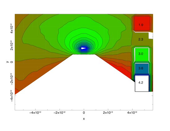
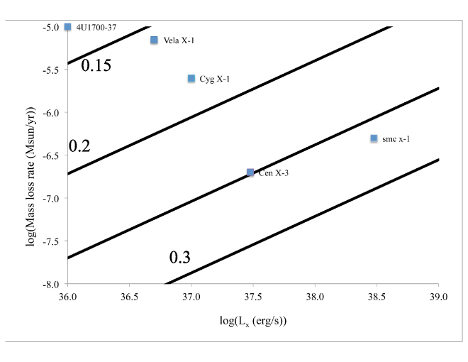
With these quantities we can use our spherical wind models to crudely predict the polarization fractions and orbital phase modulation of the polarization for these sources. We do this in the following way: we use the results in table 1 to construct an approximate scaling of mid-eclipse net polarization with the wind mass loss rate and X-ray luminosity. We then apply this to the known HMXBs in table 1. The results are shown graphically in figure 14. The most relevant quantities for each of the table 1 HMXBs, X-ray luminosity and wind mass-loss rate, are plotted on the axes and the values for each object are plotted as points. Contours of constant predicted mid-eclpise polarization are shown as solid curves, and labeled. This shows that high polarizations are expected for some objects, those with the strongest winds and weakest X-rays generally. This demonstrates that polarization fractions in the range from 5 – 30 $\%$ are expected at mid-eclipse for these systems. More detailed information is contained in the spectra and the time variation of the net polarization during eclipse; interpretation of these signals requires modeling which is tailored to each particular system.

Table 1Hydrodynamic Model Results. Values for the polarization fraction are given for several hydrodynamic models described in the text.

Model	$\dot{M}$	Lx	Pϕ=0.5
	$M_{\odot}{\rm yr}^{-1}$	erg s-1
1	4 $\times 10^{-7}$	1038	0.25
2	4 $\times 10^{-7}$	1037	0.25
3	4 $\times 10^{-7}$	1039	0.29
4	1.7 $\times 10^{-6}$	1038	0.22

Table 2Sample HMXBs and Properties Needed for Predicting Wind Polarization.

object	Sp. type	$\dot{M}_{wind}$	Lx
		$M_{\odot}{\rm yr}^{-1}$	erg s-1
Vela X-1	B0.5 Iab	7 $\times 10^{-6}$	0.05
Cen X-3	O6.5 II-III	2 $\times 10^{-7}$	0.3
Cyg X-1	O9.7 Iab	2.5 $\times 10^{-6}$	0.1
4U1700-37	O6.5 Iaf+	1 $\times 10^{-5}$	0.01
smc x-1	B0.6 Iab	5 $\times 10^{-7}$	3

APPENDIX

Illustrative analytic results can be derived for an idealized HMXB system: a spherical primary star with radius $R_{\*}\simeq 10^{12}$ cm in a circular orbit with an X-ray source with separation $a\simeq 1.5R_{\*}$. We view the system from some phase angle $\Theta_{V}$ relative to the line of centers where $\Theta_{V}=0$ corresponds to superior conjunction of the X-ray source. In addition, the system can have inclination $i$ defined such that $i=\pi/2$ corresponds to viewing in the orbital plane. The X-ray source has a luminosity $L_{X}\simeq 10^{37}$ erg s^-1 and illuminates the primary star and wind isotropically. The wind has a mass loss rate $\dot{M}\simeq 10^{-8}M_{\odot}$ yr^-1, a terminal velocity $v_{\infty}\simeq 10^{8}$cm s^-1, and a velocity law $v(r)$ which depends only on the distance from the center of the star. If so, the effects of scattering in the wind depend on the wind column density, which can be characterized by the column density $N=\int_{a}^{\infty}n(r)dr$ and an approximate value for this is $N=n_{x}a$ where $n_{x}=\frac{\dot{M}/\mu m_{H}}{4\pi a^{2}v}$ is the density at the X-ray source, $\mu$ is the mean particle weight, and $m_{H}$ is the hydrogen mass. For the fiducial parameters given above, $n_{x}=3.2\times 10^{8}$ cm^-3 $\dot{M}_{8}v_{8}^{-1}a_{12}^{-2}$ and $N=3.2\times 10^{20}$ cm^-2 $\dot{M}_{8}v_{8}^{-1}a_{12}^{-1}$. The ratio of the total intensity of scattered radiation to the total emitted radiation can be characterized by the quantity $L_{scatt}/L_{X}\sim N\sigma\simeq 2\times 10^{-4}\sigma/\sigma_{Th}\dot{M}_{8}v_{8}^{-1}a_{12}^{-1}$ where $\sigma$ is a characteristic scattering cross section and $\sigma_{Th}$ is the Thomson cross section.

We consider a coordinate system in which the observer is along the $\hat{\bf y}$ axis. Then the scattering plane is perpendicular to the (x,z) plane. We can rewrite equation 1 as:

$$\left\{\begin{matrix}L\\ Q\\ U\end{matrix}\right\}=L_{0}\sigma\int dV\frac{n({\bf r})}{r_{x}^{2}}\left\{\begin{matrix}1+\cos^{2}\chi\\ \sin^{2}\chi\cos(2\gamma)\\ \sin^{2}\chi\sin(2\gamma)\end{matrix}\right\}$$ (1)

For the purposes of computation, a more convenient expression is in terms of cylindrical coordinates centered on the X-ray source, with the observer on the axis at infinity:

$$\left\{\begin{matrix}L\\ Q\\ U\end{matrix}\right\}=L_{0}\sigma\int_{0}^{2\pi}d\gamma\int_{0}^{\infty}pdp\int_{-\infty}^{\infty}d\zeta\frac{n({\bf r})}{(p^{2}+\zeta^{2})^{2}}\left\{\begin{matrix}(p^{2}+2\zeta^{2})\\ p^{2}cos(2\gamma)\\ p^{3}sin(2\gamma)\end{matrix}\right\}$$ (2)

where $(p,\gamma,\zeta)$ are the radial, angular and axial cylindrical coordinates with the axis along y. These are indicated on figure 1. In the case a star located at a distance $a$ from the X-ray source, orbiting in a plane with a normal which is inclined at an agle $i$ with respect to line of sight, and with an orbital phase described by an angle $\theta_{v}$, this expression can be rewritten in terms of coordinates centered on the star:

$$p=r((x\cos\theta_{v}+(y+\alpha)\sin\theta_{v})^{2}+(z\sin i+(y+\alpha)\cos\theta_{v}-x\sin\theta_{v})\cos i)^{2})^{1/2}$$ (3)

$$\gamma={\rm tan}^{-1}\left(\frac{z\sin i+(y+\alpha)\cos\theta_{v}-x\sin\theta_{v})\cos i}{x\cos\theta_{v}+(y+\alpha)\sin\theta_{v}}\right)$$ (4)

$$\zeta=-r((y+\alpha)\cos\theta_{v}-x\sin\theta_{v})\sin i+z\cos i$$ (5)

where $x,y,z$ are cartesian coordinates centered on the star $r$ is the distance from the center of the star and $\alpha=a/r$. This can be evaluated analytically for special cases.

In the case of a single star, $a$=0, $\theta_{v}$=0, and if the density distribution is axially symmetric, Brown & McLean (1977) have shown that

$$\left\{\begin{matrix}L\\ Q\\ U\end{matrix}\right\}=L_{0}\sigma\int_{0}^{\infty}dr\int_{-1}^{1}\sin\theta d\theta n(r,\theta)\left\{\begin{matrix}2(1+\cos^{2}\theta)+\sin^{2}i(1-3\cos^{2}\theta)\\ \sin^{2}i(1-3\cos^{2}\theta)\\ 0\end{matrix}\right\}$$ (6)

so that the fraction varies from zero for zero inclination to a maximum value determined by the departure of the density distribution from spherical.

From equation 2 it is apparent that, in the case where the density is independent of $\gamma$, the net polarization is zero and the surfaces of constant polarization in the integrand are circular. This is expected to be the case for a binary system where the gas density is circularly symmetric around the line of centers, and when viewed at conjunction from the orbital plane (i.e. $\theta_{v}$=0 or $\pi$/2 and $i$=$\pi/2$). In the case of a binary system viewed along the angular momentum axis, i.e. $i$=0, the intensities can be shown to be:

$$\left\{\begin{matrix}L\\ Q\\ U\end{matrix}\right\}=\left\{\begin{matrix}\mathcal{I}_{0}\\ \mathcal{I}_{1}\cos 2\theta_{v}+{\mathcal{I}_{2}\sin}2\theta_{v}\\ \mathcal{I}_{1}\sin 2\theta_{v}+{\mathcal{I}_{2}\cos}2\theta_{v}\end{matrix}\right\}$$ (7)

where

$$\mathcal{I}_{0}=L_{0}\sigma\int_{0}^{\infty}r^{2}dr\int_{0}^{\pi}\sin\theta d\theta n(r,\theta,\phi)\frac{1}{(r^{2}+2ar\sin\theta\sin^{2}\phi+a^{2})}$$ (8)

$$\mathcal{I}_{1}=L_{0}\sigma\int_{0}^{\infty}r^{2}dr\int_{0}^{\pi}\sin\theta d\theta n(r,\theta,\phi)\frac{(r^{2}\sin^{2}\theta\cos^{2}\phi-(r\sin\theta\sin\phi+a)^{2})}{(r^{2}+2ar\sin\theta\sin^{2}\phi+a^{2})^{2}}$$ (9)

$$\mathcal{I}_{2}=L_{0}\sigma\int_{0}^{\infty}r^{2}dr\int_{0}^{\pi}\sin\theta d\theta n(r,\theta,\phi)\frac{r^{2}\sin^{2}\theta\sin\phi\cos\phi}{(r^{2}+2ar\sin\theta\sin^{2}\phi+a^{2})^{2}}$$ (10)

and $\mathcal{I}_{2}=0$ by symmetry if the density distribution is independent of $\phi$. This clearly represents a circle in the $(Q,U)$ plane. This, plus more general cases, were explored by Brown et al. (1978).

In the case of a binary viewed from within the orbital plane, it is straightforward to show that the polarization is zero at phases 0 and 0.5, i.e. superior and inferior conjunction of the X-ray source. At phase 0.25 or 0.75, i.e. quadrature, the stokes quantities can be written:

$$\left\{\begin{matrix}L\\ Q\\ U\end{matrix}\right\}=\frac{L_{0}\sigma\pi}{8a}\int_{0}^{\infty}rdrn(r)\left\{\begin{matrix}(18r^{2}+15a^{2}-\frac{r^{4}}{a^{2}})\frac{4ar}{(r^{2}-a^{2})^{2}}-\frac{4r}{a}+(\frac{2r^{2}}{a^{2}}-6){\rm ln}\left(\frac{r+a}{r-a}\right))\\ (22r^{2}+19a^{2}+\frac{9r^{4}}{a^{2}})\frac{4ar}{(r^{2}-a^{2})^{2}}+\frac{36r}{a}-(\frac{18r^{2}}{a^{2}}+26){\rm ln}\left(\frac{r+a}{r-a}\right))\\ 0\end{matrix}\right\}$$ (11)

This can be evaluated analytically in the limit that the density distribution is a thin shell at $r=r_{*}$ in which case the net polarization $Q/L$ varies from unity for $a>>r_{*}$ to 0.886 for $a=r_{*}$

References

- Al-Malki et al. (1999) Al-Malki, M. B., Simmons, J. F. L., Ignace, R., Brown, J. C., & Clarke, D. 1999, A&A, 347, 919
- Angel (1969) Angel, J. R. P. 1969, ApJ, 158, 219
- Blondin & Pope (2009) Blondin, J. M., & Pope, T. C. 2009, ApJ, 700, 95
- Blondin et al. (1990) Blondin, J. M., Kallman, T. R., Fryxell, B. A., & Taam, R. E. 1990, ApJ, 356, 591
- Blondin (1994) Blondin, J.M. 1994, ApJ, 435, 756
- Bondi & Hoyle (1944) Bondi, H., & Hoyle, F. 1944, MNRAS, 104, 273
- Brown & McLean (1977) Brown, J. C., & McLean, I. S. 1977, A&A, 57, 141
- Brown et al. (1978) Brown, J. C., McLean, I. S., & Emslie, A. G. 1978, A&A, 68, 415
- Rudy & Kemp (1978) Rudy, R. J., & Kemp, J. C. 1978, ApJ, 221, 200
- Castor (1970) Castor, J.I., 1970, MNRAS, 149, 111
- Castor et al. (1975) Castor, J. I., Abbott, D. C., Klein, R. I. 1975, ApJ, 195, 157
- Chandrasekhar (1960) Chandrasekhar, S. 1960, Radiative transfer, Dover, New York
- Clark et al. (1988) Clark, G. W., Minato, J. R., & Mi, G. 1988, ApJ, 324, 974
- Cohen et al. (2006) Cohen, D. H., Leutenegger, M. A., Grizzard, K. T., et al. 2006, MNRAS, 368, 1905
- Conti (1978) Conti, P. S. 1978, A&A, 63, 225
- Costa et al. (2006) Costa, E., et al. 2006, Proc. SPIE, 6266,
- Davidson & Ostriker (1973) Davidson, K., & Ostriker, J. P. 1973, ApJ, 179, 585
- Dorodnitsyn & Kallman (2010) Dorodnitsyn, A., & Kallman, T. 2010, ApJL 711, 112
- Fabbiano (2006) Fabbiano, G. 2006, ARA&A, 44, 323
- Fransson & Fabian (1980) Fransson, C., & Fabian, A. C. 1980, A&A, 87, 102
- Hamilton (1947) Hamilton, D. 1947, ApJ, 106, 457
- Hatchett & McCray (1977) Hatchett, S., & McCray, R. 1977, ApJ, 211, 552
- Ignace et al. (2009) Ignace, R., Al-Malki, M. B., Simmons, J. F. L., et al. 2009, A&A, 496, 503
- Jahoda et al. (2014) Jahoda, K. M., Black, J. K., Hill, J. E., et al. 2014, Proc. SPIE, 9144, 91440N
- Kallman & McCray (1982) Kallman, T. R., & McCray, R. 1982, ApJS, 50, 263
- Kallman & Bautista (2001) Kallman, T., Bautista, M. 2001, ApJS, 133, 221
- Kaper (1998) Kaper, L. 1998, Properties of Hot Luminous Stars, 131, 427
- Lamb et al. (1973) Lamb, F. K., Pethick, C. J., & Pines, D. 1973, ApJ, 184, 271
- Lamers & Cassinelli (1999) Lamers, H. J. G. L. M., & Cassinelli, J. P. 1999, Introduction to Stellar Winds, by Henny J. G. L. M. Lamers and Joseph P. Cassinelli, pp. 452. ISBN 0521593980. Cambridge, UK: Cambridge University Press, June 1999.,
- Lee et al. (1994) Lee, H.-W., Blandford, R.D., Western, L. 1994, MNRAS, 267, 303
- Liu et al. (2006) Liu, Q. Z., van Paradijs, J., & van den Heuvel, E. P. J. 2006, A&A, 455, 1165
- Lucy & White (1980) Lucy, L.B., White, R.L. 1980, ApJ, 241, 300
- Matt et al. (1996) Matt, G., Feroci, M., Rapisarda, M., & Costa, E. 1996, Radiation Physics and Chemistry, 48, 403
- Matt (2004) Matt, G. 2004, A&A, 423, 495
- Mauche et al. (2008) Mauche, C. W., Liedahl, D. A., Akiyama, S., & Plewa, T. 2008, American Institute of Physics Conference Series, 1054, 3
- McNamara et al. (2008) McNamara, A. L., Kuncic, Z., & Wu, K. 2008, MNRAS, 386, 2167
- Meszaros et al. (1988) Meszaros, P., Novick, R., Szentgyorgyi, A., Chanan, G. A., & Weisskopf, M. C. 1988, ApJ, 324, 1056
- Mihalas (1978) Mihalas, D. 1978, San Francisco, W. H. Freeman and Co., 1978. 650 p.,
- Nofi & Wiktorowicz (2014) Nofi, L., & Wiktorowicz, S. 2014, American Astronomical Society Meeting Abstracts 224, 224, 219.21
- Owocki et al. (1988) Owocki S. P., Castor J. I., Rybicki G. B., 1988, ApJ, 335, 914
- Taam & Sandquist (2000) Taam, R. E., & Sandquist, E. L. 2000, ARA&A, 38, 113
- Tarter et al. (1969) Tarter, C.B., Tucker, W., Salpeter, E.E. 1969, ApJ, 156, 943
- van der Meer et al. (2007) van der Meer, A., Kaper, L., van Kerkwijk, M. H., Heemskerk, M. H. M., & van den Heuvel, E. P. J. 2007, A&A, 473, 523
- van Paradijs (1995) van Paradijs, J. 1995, X-ray binaries, p. 536 - 577, 536
- Walter et al. (2015) Walter, R., Lutovinov, A. A., Bozzo, E., & Tsygankov, S. S. 2015, A&A Rev., 23, 2
- Watanabe et al. (2006) Watanabe, S., et al. 2006, ApJ, 651, 421
- Weisskopf et al. (1978) Weisskopf, M. C., Silver, E. H., Kestenbaum, H. L., Long, K. S., & Novick, R. 1978, ApJ, 220, L117
- Weisskopf et al. (2013) Weisskopf, M. C., Baldini, L., Bellazini, R., et al. 2013, Proc. SPIE, 8859, 885908
- White (1985) White, N. E. 1985, NATO ASIC Proc. 150: Interacting Binaries, 249