Influence of external forcings on abrupt millennial-scale climate changes: a statistical modelling study

Abstract

The last glacial period was punctuated by a series of abrupt climate shifts, the so-called Dansgaard-Oeschger (DO) events. The frequency of DO events varied in time, supposedly because of changes in background climate conditions. Here, the influence of external forcings on DO events is investigated with statistical modelling. We assume two types of simple stochastic dynamical systems models (double-well potential-type and oscillator-type), forced by the northern hemisphere summer insolation change and/or the global ice volume change. The model parameters are estimated by using the maximum likelihood method with the NGRIP Ca²⁺ record. The stochastic oscillator model with at least the ice volume forcing reproduces well the sample autocorrelation function of the record and the frequency changes of warming transitions in the last glacial period across MISs 2, 3, and 4. The model performance is improved with the additional insolation forcing. The BIC scores also suggest that the ice volume forcing is relatively more important than the insolation forcing, though the strength of evidence depends on the model assumption. Finally, we simulate the average number of warming transitions in the past four glacial periods, assuming the model can be extended beyond the last glacial, and compare the result with an Iberian margin sea-surface temperature (SST) record (Martrat et al., Science, vol. 317, p. 502, 2007). The simulation result supports the previous observation that abrupt millennial-scale climate changes in the penultimate glacial (MIS 6) are less frequent than in the last glacial (MISs 2–4). On the other hand, it suggests that the number of abrupt millennial-scale climate changes in older glacial periods (MISs 6, 8, and 10) might be larger than inferred from the SST record.

1 Introduction

During the last glacial period, the North Atlantic region experienced a series of abrupt climate shifts between cold (stadial) and relatively warm (interstadial) phases, the so-called Dansgaard-Oeschger (DO) events (Dansgaard et al, 1993). These are clearly reflected in changes in the oxygen isotope ratio $\delta^{18}$O${}_{\text{ice}}$ (a proxy for air temperature) of Greenland ice cores (see Fig. 1(b)). Typically, abrupt warmings occurred within a few decades, and they were followed by a gradual cooling before a rapid return to a cold state. The amplitude of the abrupt warmings ranges from $8^{\circ}$C to $16^{\circ}$C (Wolff et al (2010) and references therein).

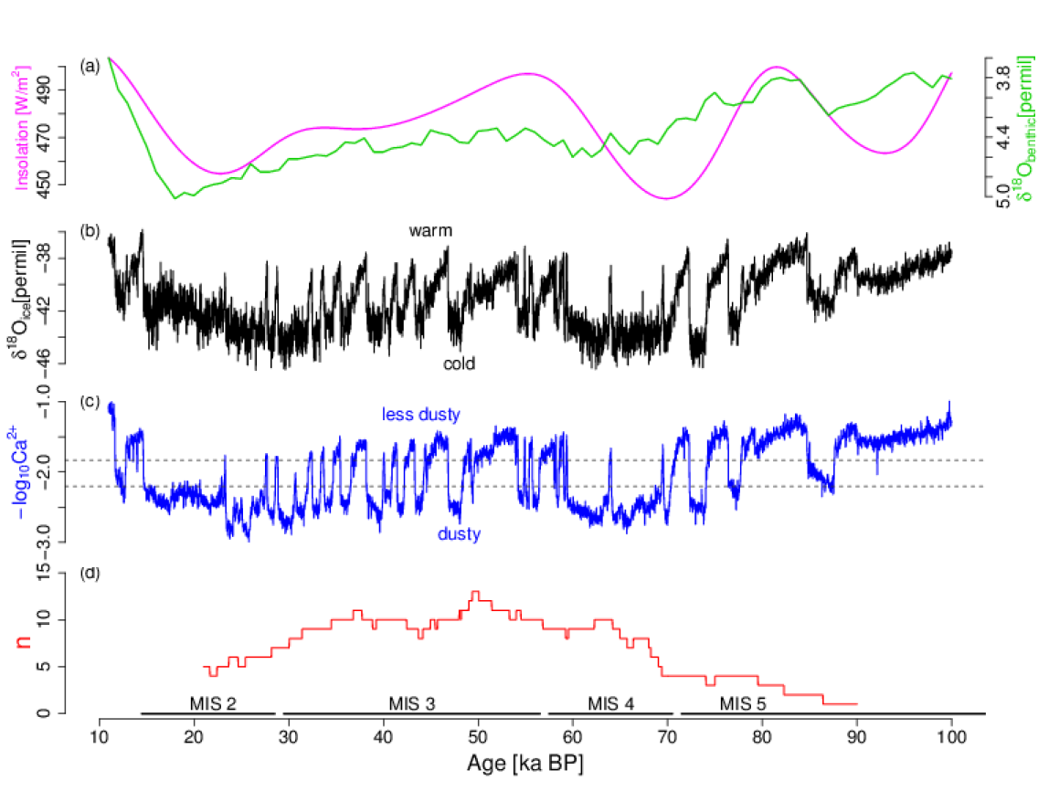
Figure 1: Comparison between NGRIP ice core records and background climate conditions. (a) The mean monthly insolation from 21 June to 20 July at 65^∘N (magenta) (Laskar et al, 2004) and the benthic oxygen isotope ratio $\delta^{18}$O${}_{\text{benthic}}$ as a proxy for the global ice volume (green) (Lisiecki and Raymo, 2005). (b) The 20-year average NGRIP $\delta^{18}$O${}_{\text{ice}}$ (Rasmussen et al, 2014). (c) The 20-year average NGRIP Ca²⁺ concentration (ppb) (blue) (Rasmussen et al, 2014). The dashed lines are the upper and lower thresholds used to define a warming transition. (d) The number of warming transitions $n(t)$ for each moving time window [$t-10$ ka, $t+10$ ka]. The marine isotope stages (MISs) are based on Lisiecki and Raymo (2005).

DO events are commonly associated with changes in deep-ocean activity and sea-ice cover in the North Atlantic (Gildor and Tziperman, 2003; Denton et al, 2005; Li et al, 2005). They are also associated with changes in the large scale thermohaline circulation (THC) (Broecker et al, 1985; Rahmstorf, 2002), though such circulation changes do not seem as dramatic as those that occurred during Heinrich events (Elliot et al (2002); Clement and Peterson (2008) and references threrein). What causes the onset, demise, and recurrence of DO events is still not so clear (Clement and Peterson, 2008). A number of modelling studies show that the convective activity and the broader THC depend nonlinearly on the freshwater balance of the North Atlantic (Manabe and Stouffer, 1988; Ganopolski and Rahmstorf, 2001). In turn, such circulation changes may impact the mass balance of the surrounding ice sheets and their freshwater supply onto the ocean. Such interplay may explain complex dynamics of DO events (Kageyama and Paillard, 2005). Alternatively, it has been suggested that self-sustained oscillations are possible as a result of advective and convective dynamics in the ocean without any change in freshwater input (for example, Colin de Verdière (2007)).

Greenland ice cores contain various continental dusts transported from mainly East Asian deserts (Biscaye et al, 1997). There is a strong correlation between $\delta^{18}$O${}_{\text{ice}}$ (Fig. 1(b)) and dust concentrations (approximated by [Ca²⁺], Fig. 1(c)) in the ice cores. This suggests that North Atlantic climate changes are tightly linked with changes in northern hemisphere atmospheric circulation (Mayewski et al, 1997) or dust storm activity in East Asia (Ruth et al, 2007). A recent simulation shows that the increase in the meridional temperature gradient in the North Atlantic leads to stronger westerlies (important for long-range dust transport) and strengthened winter wind speed above major Asian dust source regions (important for dust entrainment) (Sun et al, 2012).

The occurrence frequency of DO events varied in time as shown in Fig. 1. The frequency is quantified by counting the number of warming transitions $n(t)$ for each 20-ka moving window [$t-10$ ka, $t+10$ ka] over the 20-year average NGRIP Ca²⁺ record (Rasmussen et al, 2014). Here, we standardize $-\log_{10}[\text{Ca}^{2+}]$ by the mean and standard deviation during 11–100 ka BP as $y=(-\log_{10}[\text{Ca}^{2+}]+2.02)/0.464$. A warming transition is then defined as the first up-crossing of the upper threshold $y=0.4$ after falling below the lower threshold $y=-0.4$ (dashed lines in Fig. 1(c)). The number of warming transitions $n(t)$ increases from MIS 5 to MIS 3 and decreases from MIS 3 to MIS 2 (Fig. 1(d)). The purpose of this paper is to explore external forcings which induce these frequency changes.

Ice sheet forcing. The millennial-scale climate changes have larger amplitudes when the global ice volume is in intermediate level (McManus et al, 1999). Northern hemisphere ice sheets may affect the THC or the sea ice formation in the North Atlantic by their meltwater discharges (Schulz et al, 2002; Knutti et al, 2004; Jackson et al, 2010), by changing wind fields (Wunsch, 2006), or by their albedo effect. Using a comprehensive climate model, Zhang et al (2014) show that small changes of the height of the northern hemisphere ice sheets can cause rapid climate transitions like DO events via an atmosphere-ocean-sea-ice feedback in the North Atlantic.

Astronomical insolation forcing. The seasonal and latitudinal distribution of the insolation at the top of the atmosphere varies due to the long term variations of the Earth’s astronomical parameters: climatic precession, obliquity, and eccentricity (Berger and Loutre, 1991). Several observational as well as modelling studies propose the influence of boreal summer insolation change (Fig. 1(a)) on DO events (Adams et al, 1999; Martrat et al, 2004; Rial and Yang, 2007; Capron et al, 2010). On the other hand, Masson-Delmotte et al (2005); Olsen et al (2005); Friedrich et al (2010) emphasize the influence of the latitudinal gradient of annual mean insolation (i.e., obliquity forcing).

CO₂ forcing. The atmospheric CO₂ concentration varied in a range of 180–280 ppm over the last four glacial cycles (Petit et al, 1999). Increases of CO₂ by $\sim$20 ppm are observed prior to large DO warmings after Heinrich events (Ahn and Brook, 2008). A fully coupled model simulation by Zhang et al (2014) shows an increase of CO₂ by 20 ppm (corresponding to the change in the radiative forcing by $\sim$0.55 W/m²) can trigger warming transitions like DO events.

In this study, we focus on the northern hemisphere summer insolation forcing and the ice volume forcing. The ice volume contains the information of insolation change in part (Hays et al, 1976). However, with close inspection in Fig. 1(a), these curves have only a weak correlation (the coefficient of determination $R^{2}=0.14$). The CO₂ forcing is not explicitly considered here, but it is implicitly included in the ice volume forcing because the atmospheric CO₂ concentration (in logarithmic scale) is strongly correlated to the global sea-level ($R^{2}=0.68$ over the past 550 ka (Foster and Rohling, 2013)). There is a debate on the temporal regularity of DO events. Schulz (2002a) proposed that DO events occurred with periods multiple of 1470 yr. The periodicity evoked the existence of external clock, for example, solar cycles (Braun et al, 2008) or tidal cycles (Keeling and Whorf, 2000). However, the statistical significance of 1470-yr periodicity is questioned by Ditlevsen et al (2007). He argues that the onsets of DO events are indistinguishable from a random occurrence (more precisely a Poisson process). Thus, we assume that millennial cycles are generated by stochastic dynamics without explicit 1470-yr forcing.

To infer the influence of external forcings in noisy records, we take an approach by statistical modelling based on dynamical systems, which has many paleoclimatic applications: ice ages (Hargreaves and Annan, 2002; Crucifix and Rougier, 2009), DO events (Kwasniok and Lohmann, 2009, 2012; Peavoy and Franzke, 2010; Kwasniok, 2013), and abrupt monsoon transitions (Thomas et al, 2015). As in Kwasniok (2013), we assume two types of simple dynamical systems models based on two paradigms of DO dynamics, bistability and oscillations, but here these systems are forced by the northern hemisphere summer insolation change and/or the ice volume change. In our analysis, superiority of the oscillator model and the relative importance of the ice volume forcing are shown. Finally, we simulate the abrupt millennial-scale climate changes beyond the last glacial, assuming the model can be extended, and compare the result with the Iberian margin SST record over these periods (Martrat et al, 2007).

The remainder of this article is organized as follows. In Section 2, we explain the data and methods. In Section 3, we show the results of the model parameter estimation. The calibrated models are compared in Section 4. We predict the occurrence frequency of abrupt millennial-scale climate changes in the past four glacial periods in Section 5.

2 Data and methods

2.1 Data

The calcium ion concentration [Ca²⁺] in ice cores is a proxy of continental dusts transported from mainly East Asian deserts, which depend on several factors (Fuhrer et al, 1999): (i) source area conditions (such as aridity or vegetation), (ii) mobilization of dusts by winds in source areas and uplift to transporting levels, (iii) long-range transport efficiency depending on transient times, (iv) losses en route (gravitational settling or wash-out), and (v) deposition on ice sheet. The relative contribution is a matter of debate. Fischer et al (2007) propose larger contributions of both source strength and transport, while Ruth et al (2007) propose that the increase of dust concentrations during stadials is largely attributed to the increased dust storm activity in East Asia.

The quantity $-\log_{10}$[Ca²⁺] is well correlated with $\delta^{18}$O${}_{\text{ice}}$ ($R^{2}=0.82$ in the case of Fig. 1), and it is assumed to change synchronously with the oxygen isotope ratio $\delta^{18}$O${}_{\text{ice}}$ within 20-year resolution (Rasmussen et al, 2014). There are advantages in the use of Ca²⁺ signals: Ca²⁺ has an excellent signal-to-noise ratio (Rasmussen et al, 2014), and the differences between ice cores (NGRIP, GRIP, and GISP2) are small compared to $\delta^{18}$O${}_{\text{ice}}$ (see Fig. 1 in Rasmussen et al (2014)).

We use the 20-year average NGRIP Ca²⁺ on the GICC05modelext timescale (Rasmussen et al, 2014; Bigler, 2004) standardized as $y=(-\log_{10}[\text{Ca}^{2+}]+2.02)/0.464$ by the mean and standard deviation during $11$–$100$ ka BP. To assess the proxy dependence of the result, we also use the 20-year average NGRIP oxygen isotope ratio $\delta^{18}$O${}_{\text{ice}}$ (Rasmussen et al, 2014) standardized in a similar manner.

In our models (next Subsection), we employ the mean monthly insolation from 21 June to 20 July at 65^∘N (Laskar et al, 2004) and the global ice volume estimated from the benthic oxygen isotope ratio $\delta^{18}$O${}_{\text{benthic}}$ (the LR04 stack record by Lisiecki and Raymo (2005)). The former is standardized by subtracting the mean 474.93 W/m² and dividing by standard deviation 15.08 W/m² during 11–100 ka BP. This is referred to as the insolation forcing $I(t)$. The LR04 stack record is linearly interpolated to have $20$-yr resolution and then standardized with the mean 4.34 $\permil$ and standard deviation 0.33 $\permil$. This is referred to as the ice volume forcing $V(t)$. $\delta^{18}$O${}_{\text{benthic}}$ is affected both by the global ice volume and deep water temperature, but we use $\delta^{18}$O${}_{\text{benthic}}$ as a rough approximation of the global ice volume change.

2.2 Models

Given that the mechanism of DO events is still in debate, we assume simple abstract dynamical models: a stochastic one-dimensional (1D) potential model and a stochastic oscillator model (Kwasniok, 2013). The way to include the forcings $I(t)$ and $V(t)$ in the models is not obvious. As the simplest assumption, we assume that the system is linearly forced by $I(t)$ and $V(t)$ with relative weights $\gamma_{1}$ and $\gamma_{2}$.

2.2.1 Stochastic 1D potential model

The most prevalent hypothesis is that DO events are the transitions between two climate states corresponding to “warm” and “cold” modes of the THC (Broecker et al, 1985; Rahmstorf, 2002). Denote the model’s “true” state for the standardized $-\log_{10}$[Ca²⁺] by $x(t)$. The bistability hypothesis can be expressed by the following stochastic dynamical systems model:

$$\begin{split}&dx(t)=[-U^{\prime}(x)+\gamma_{1}I(t)-\gamma_{2}V(t)]dt+\sigma dW(t),\\ &U(x)=a_{1}x+a_{2}x^{2}+a_{3}x^{3}+a_{4}x^{4},\,\,\,a_{4}>0,\end{split}$$ (1)

where $\sigma dW(t)$ is the system noise and $W(t)$ is the standard Wiener process (Gardiner, 2009). The infinitesimal increment $dW(t)=W(t+dt)-W(t)$ obeys a normal distribution $\mathcal{N}(0,dt)$ with mean zero and variance $dt$. The 4th order potential $U(x)$ is a minimal model which allows bimodality. Equations similar to (1) have been used to describe the dynamics of THC (Stommel and Young, 1993; Cessi, 1994; Timmermann and Lohmann, 2000; Vé1ez-Belchí et al, 2001; Monahan, 2006), DO events (Ditlevsen, 1999; Kwasniok and Lohmann, 2009; Rial and Saha, 2011), or abrupt monsoon transitions (Thomas et al, 2015).

The measurement $y(t)$ obeys the following observation model:

$$y(t)=x(t)+\eta(t),\,\,\,\eta(t)\sim\mathcal{N}(0,\varepsilon^{2}).$$ (2)

The observation noise $\eta(t)$ includes all the discrepancies between the model state and the measurement (i.e., instrument errors and representation errors). It is modeled by a white noise obeying a normal distribution $\mathcal{N}(0,\varepsilon^{2})$. In addition to this original model with 8 parameters, we consider a submodel with 7 parameters obtained by setting $\varepsilon\equiv 0$. We refer to the original model as the 1D potential model A and the submodel as the 1D potential model B.

2.2.2 Stochastic oscillator model

The second paradigm of DO events is based on self-sustained oscillations (Broecker et al, 1990), which appear in simple conceptual models (Birchfield and Broecker, 1990; Winton, 1993; Sakai and Peltier, 1999; Rial and Saha, 2011), Earth System Models of Intermediate Complexity (EMICs) (Sakai and Peltier, 1997; Wang and Mysak, 2006; Friedrich et al, 2010), and coupled GCMs (Peltier and Vettoretti, 2014). Many works involve instabilities of the THC (possibly coupled with sea ice) as a mechanism of oscillations, while an instability in atmosphere–ocean–ice–sheet system is also proposed (Kageyama and Paillard, 2005).

The third paradigm is related to excitability. Ganopolski and Rahmstorf (2001) explain DO events by two modes of THC with different convection sites, where the cold mode is stable and the warm mode is marginally unstable. Coherent oscillations between these two modes arise when the freshwater perturbations have an optimal magnitude (Ganopolski and Rahmstorf, 2002).

The FitzHugh-Nagumo model (also known as Bonhoeffer–van der Pol oscillator) is a paradigmatic model, which can exhibit both self-sustained oscillations and excitability (FitzHugh, 1961; Nagumo et al, 1962). A particular case of FitzHugh-Nagumo model is introduced as a model of DO events by Kwasniok (2013). Here, we consider a forced version of Kwasniok’s model:

$${\ddot{x}}+[\alpha+\beta(x-x_{*})^{2}]{\dot{x}}+k(x-x_{0})=\gamma^{\prime}_{0}+\gamma^{\prime}_{1}I(t)-\gamma^{\prime}_{2}V(t).$$ (3)

where the parameters $x_{*}$ and $x_{0}$ control dissipative and linear restoring forces, respectively, and the parameter $\gamma_{0}^{\prime}$ is the bias of the external forcing. A priori, $\alpha$ can be either positive or negative. The condition $\alpha<0$ is necessary to exhibit self-sustained oscillations.

By the Liénard transformation $v=({\dot{x}}+\int_{0}^{x}[\alpha+\beta(x-x_{*})^{2}]dx)/k$ and by adding stochastic forcing terms, we obtain

$$dx(t)=\left\{kv-\alpha x-\frac{\beta}{3}[(x-x_{*})^{3}+x_{*}^{3}]\right\}dt+\sigma_{1}dW_{1}(t),$$ (4)

$$dv(t)=\left\{-x+\gamma_{0}+\gamma_{1}I(t)-\gamma_{2}V(t)\right\}dt+\sigma_{2}dW_{2}(t),$$ (5)

where $\gamma_{0}=\gamma_{0}^{\prime}/k+x_{0}$, $\gamma_{1}=\gamma^{\prime}_{1}/k$, and $\gamma_{2}=\gamma^{\prime}_{2}/k$, and $W_{1}(t)$ and $W_{2}(t)$ are mutually independent Wiener processes. Again, $x(t)$ is the model’s true state for the standardized $-\log_{10}$[Ca²⁺], and the observation model is given by Eq. (2). In addition to this original model with 10 parameters, we also consider a submodel with 9 parameters obtained by setting $\sigma_{1}\equiv 0$. We refer to the original model as the oscillator model A and the submodel as the oscillator model B.

2.3 State and parameter estimation

The parameter estimation is performed jointly with the state estimation.

2.3.1 State estimation

The state estimation is here performed with the Unscented Kalman filter (UKF) (Julier and Uhlmann, 2004). Here, we describe the procedure of the UKF for the oscillator model given by Eqs. (4), (5), and (2), but the application for the 1D potential model is straightforward. With the Euler-Maruyama method (Gardiner (2009), p. 404), Eqs. (4), (5), and (2) can be written in a recursive form:

$$\begin{split}\mathbf{x}(t+h)&=\mathbf{f}(\mathbf{x}(t),t)+\mathbf{q}(t),\,\,\,\mathbf{q}(t)\sim\mathcal{N}(0,\mathbf{Q}),\\ y(t+h)&=\mathbf{H}\mathbf{x}(t+h)+\eta(t+h),\\ \mathbf{f}(\mathbf{x}(t),t)&=\mathbf{x}(t)+\begin{pmatrix}kv-\alpha x-\frac{\beta}{3}[(x-x_{*})^{3}+x_{*}^{3}]\\ -x+\gamma_{0}+\gamma_{1}I(t)-\gamma_{2}V(t)\\ \end{pmatrix}h,\end{split}$$ (6)

where $h$ is a time step, $\mathbf{x}(t)=(x(t),v(t))^{T}\in\mathbf{R}^{m}$ is a $m$-dimensional state vector ($m=2$ for the oscillator model), $y(t)$ is a scalar observation variable obtained by the operation of observation matrix $\mathbf{H}=(1\,0)$, and $\mathcal{N}(0,\mathbf{Q})$ is the zero mean multivariate normal distribution with covariance matrix

$$\mathbf{Q}=\begin{pmatrix}h\sigma_{1}^{2}&0\\ 0&h\sigma_{2}^{2}\\ \end{pmatrix}.$$

Assume $N$ measurements $y_{k}=y(t_{k})$ ($k=1,\,2,...,N$) obtained at $t_{k}=t_{0}+k\Delta T$ in the time interval of $\Delta T$($\geq h$). Denote the measurements up to $k$ by $y_{1:k}=\{y_{1},y_{2},...,y_{k}\}$. The purpose of filtering is to obtain the conditional probability density $p(\mathbf{x}(t_{k})|y_{1:k})$ given the measurements up to $k$ (so-called filtered density). The Kalman filter provides exact solutions to the filtering problems in particular cases of linear models with Gaussian densities. For nonlinear models, the Kalman filter is not available because the filtered density $p(\mathbf{x}(t_{k})|y_{1:k})$ deviates from Gaussian. The unscented Kalman filter (UKF) is one extension of the Kalman filter for nonlinear models, where the filtered density $p(\mathbf{x}(t_{k})|y_{1:k})$ is approximated by a Gaussian distribution with consideration for the effect of nonlinear transformations (Julier and Uhlmann, 2004). As a result, the filtered density $p(\mathbf{x}(t_{k})|y_{1:k})$ is specified only by its mean $\hat{\mathbf{x}}_{k|k}$ (the filtered mean) and covariance $\mathbf{P}_{k|k}$ (the filtered covariance). The details for implementing the UKF are presented, for example, in Kwasniok and Lohmann (2012), but we repeat them here for self-consistency:

Assume the mean $\hat{\mathbf{x}}_{0|0}$ and covariance $\mathbf{P}_{0|0}$ of the initial density $p(\mathbf{x}(t_{0})|y_{1:0})$, where $y_{1:0}$ is the null set since we have no measurement at $t_{0}$. The time interval $[t_{k-1},t_{k}]$ between successive measurements is divided into $L=\Delta T/h$ subintervals.

Prediction step. Assume that we have calculated the filtered mean and the filtered covariance up to $\hat{\mathbf{x}}_{k-1|k-1}$ and $\mathbf{P}_{k-1|k-1}$. We sequentially calculate a predicted mean $\hat{\mathbf{x}}_{l}$ and a predicted covariance $\mathbf{P}_{l}$ at time $t=t_{k-1}+lh$ up to $l=L$, starting with $\hat{\mathbf{x}}_{0}=\hat{\mathbf{x}}_{k-1|k-1}$ and $\mathbf{P}_{0}=\mathbf{P}_{k-1|k-1}$. First, we generate an ensemble of state points, which has the same mean and covariance as $\hat{\mathbf{x}}_{l-1}$ and $\mathbf{P}_{l-1}$, the so-called sigma points:

$$\bm{\chi}^{i}_{l-1|l-1} = \hat{\mathbf{x}}_{l-1}-(\sqrt{m\mathbf{P}_{l-1}})_{i},$$

$$\bm{\chi}^{i+m}_{l-1|l-1} = \hat{\mathbf{x}}_{l-1}+(\sqrt{m\mathbf{P}_{l-1}})_{i},\,\,\,i=1,...,m,$$ (7)

where $(\cdot)_{i}$ means the $i$th column of a matrix and the square root matrix $\sqrt{m\mathbf{P}_{l-1}}$ is obtained by the Choleski decomposition of $m\mathbf{P}_{l-1}$. Each sigma point $\bm{\chi}^{i}_{l-1|l-1}$ is propagated by the deterministic part of Eq. (6):

$$\bm{\chi}^{i}_{l|l-1}=\mathbf{f}(\bm{\chi}^{i}_{l-1|l-1},t_{k}+(l-1)h).$$

Then, the predicted mean $\hat{\mathbf{x}}_{l}$ and the predicted covariance $\mathbf{P}_{l}$ at time $t=t_{k-1}+lh$ are given as

$$\hat{\mathbf{x}}_{l}=\frac{1}{2m}\sum_{i=1}^{2m}\bm{\chi}^{i}_{l|l-1},\,\,\,\mathbf{P}_{l}=\frac{1}{2m}\sum_{i=1}^{2m}(\bm{\chi}^{i}_{l|l-1}-\hat{\mathbf{x}}_{l})(\bm{\chi}^{i}_{l|l-1}-\hat{\mathbf{x}}_{l})^{T}+\mathbf{Q}.$$

If we reach $l=L$, we go to the following filtering step setting $\hat{\mathbf{x}}_{k|k-1}=\hat{\mathbf{x}}_{L}$ and $\mathbf{P}_{k|k-1}=\mathbf{P}_{L}$.

Filtering step. The filtered mean $\hat{\mathbf{x}}_{k|k}$ and the filtered covariance $\mathbf{P}_{k|k}$ are given by the usual Kalman filter equation:

$$\begin{split}\hat{\mathbf{x}}_{k|k}&=\hat{\mathbf{x}}_{k|k-1}+\mathbf{K}_{k}\mathbf{\zeta}_{k},\\ \mathbf{P}_{k|k}&=(\mathbf{I}-\mathbf{K}_{k}\mathbf{H})\mathbf{P}_{k|k-1},\\ \mathbf{\zeta}_{k}&=y_{k}-\mathbf{H}\hat{\mathbf{x}}_{k|k-1},\\ \mathbf{K}_{k}&=\mathbf{P}_{k|k-1}\mathbf{H}^{T}S_{k}^{-1},\\ S_{k}&=\mathbf{H}\mathbf{P}_{k|k-1}\mathbf{H}^{T}+\varepsilon^{2},\end{split}$$ (8)

where $\mathbf{\zeta}_{k}$ is called the innovation, $\mathbf{K}_{k}$ is the Kalman gain matrix, and $S_{k}$ is the innovation covariance. The prediction and filtering are continued until $k=N$.

2.3.2 Parameter estimation

The likelihood is the conditional probability density of the observations $y_{1:N}$ when the model parameters $\theta$ are given: $L(\theta)=p(y_{1:N}|\theta)=\prod_{k=1}^{N}p(y_{k}|y_{1:k-1},\theta).$ Owing to the Markov property of Eq. (6) and the Gaussian approximation of the filtered density in the UKF, the log-likelihood $\ln L(\theta)$ can be written as

$$\ln L(\theta)=-\frac{N}{2}\ln 2\pi-\frac{1}{2}\sum_{k=1}^{N}\left(\ln S_{k}+\frac{\zeta_{k}^{2}}{S_{k}}\right).$$ (9)

The maximum likelihood estimator (MLE) is the parameter that maximizes Eq. (9):

$$\hat{\theta}=\text{argmax}_{\theta}L(\theta)=\text{argmax}_{\theta}\ln L(\theta).$$

The covariance matrix of the MLE is estimated from the hessian matrix of the log-likelihood function:

$$\text{var}(\hat{\theta})=-\left[\frac{\partial^{2}\ln L(\theta)}{\partial\theta\partial\theta^{T}}\right]_{\theta=\hat{\theta}}^{-1}.$$

We maximize the likelihood $\ln L(\theta)$ by a quasi-Newton method, called the Limited-memory Broyden-Fletcher-Goldfarb-Shanno (L-BFGS-B) method (Byrd et al, 1994) implemented in the R-function optim (R Development Core Team, 2008). The L-BFGS-B method allows physically-reasonable constraints on the parameter regions (such as $a_{4}>0$ and $\beta>0$). This procedure may be interpreted as the implementation of bounded uniform priors in a Bayesian framework. To find the global maximum of $\ln L(\theta)$ (not just a local one), we maximize $\ln L(\theta)$ starting from several different values of $\theta$ sampled from an enough wide parameter region.

We note that sequential Monte-Carlo algorithms exist to estimate the likelihood without the possible biases introduced by the Gaussian approximations used in the UKF (Andrieu et al, 2010; Chopin et al, 2013). In a separate study, Carson et al (2015) show that such algorithms may even be implemented to estimate model evidence (Bayes factors, see Section 2.4) in paleoclimate applications, but such algorithms are more computationally expensive. We leave a more systematic comparison of the different algorithms for a future study.

2.4 Model comparison method

The models are compared using several diagnostics: the probability density, the sample autocorrelation function (Venables and Ripley, 2013), the occurrence frequency of DO warmings $n(t)$ defined in Section 1, and the Bayesian Information Criterion (BIC). Here, we outline the BIC.

In Bayesian model selection, the Bayes factor $B_{ij}$ is used as a standard measure to quantify the evidence in favor of a model (say $M_{i}$) against model (say $M_{j}$):

$$B_{ij}=\frac{p(y_{1:N}|M_{i})}{p(y_{1:N}|M_{j})},$$

where the models need not be nested (Kass and Raftery, 1995). The quantity $p(y_{1:N}|M_{i})$ is the probability density of the data $y_{1:N}$ given a model $M_{i}$ and obtained as

$$p(y_{1:N}|M_{i})=\int p(y_{1:N}|\theta_{i},\,M_{i})p(\theta_{i}|M_{i})d\theta_{i},$$ (10)

where $p(y_{1:N}|\theta_{i},\,M_{i})$ is the likelihood under the model $M_{i}$ and $p(\theta_{i}|M_{i})$ is the prior density. A value of $B_{ij}>1$ means that the model $M_{i}$ is more strongly supported by the data than the model $M_{j}$. In many practical cases, the calculation of Eq. (10) is computationally expensive, and reasonable specifications of prior density $p(\theta_{i}|M_{i})$ are difficult.

One approach for evaluating Bayes factors is the Bayesian Information Criterion (BIC) (Kass and Raftery, 1995):

$$\text{BIC}=-2\ln L(\hat{\theta})+K\ln N,$$ (11)

where $K$ is the number of the model parameters, $N$ is the number of data points, and $\ln L(\hat{\theta})$ is the maximum log-likelihood. Denote the Bayesian Information Criterion for model $i$ by $\text{BIC}_{i}$. The BIC provides a useful approximation to the Bayes factor for large $N$ with a relative error of $O(N^{-1/2})$:

$$2\ln B_{ij}\approx\text{BIC}_{j}-\text{BIC}_{i}=\Delta\text{BIC}_{ij},$$ (12)

if we assume the unit information prior on the parameters (Kass and Raftery, 1995). The unit information prior is a multivariate normal prior with mean at the maximum likelihood estimator and covariance equal to the expected information matrix for one observation. This can be thought of as an uninformative prior which contains the same amount of information as a single, typical observation (Raftery, 1995). Among several models, the model with lowest BIC is preferred. The Akaike Information Criterion, $\text{AIC}=-2\ln L(\hat{\theta})+2K,$ is another popular criterion for model selection (Akaike, 1974). The BIC penalizes the number of parameters more strongly than the AIC for large $N$.

Raftery (1995) provides a rule of thumb for interpreting the BIC difference: the evidence is said weak if $0<\Delta\text{BIC}<2$, positive if $2<\Delta\text{BIC}<6$, strong if $6<\Delta\text{BIC}<10$, and very strong if $\Delta\text{BIC}>10$. In most cases, the BIC difference is more conservative than the Bayes factors based on more informative priors (Raftery, 1999); That is, if the BIC difference shows evidence, the Bayes factors based on more informative priors are likely to show evidence. Thus, Raftery (1999) recommends to use the BIC difference as a baseline reference quantity. In this study, we have little prior knowledge on parameters, and hence report only the BIC difference as an element of model evidence.

3 Results: parameter estimation

The 1D potential models (A and B) and the oscillator models (A and B) are respectively studied for four cases: no forcing ($\gamma_{1}\equiv\gamma_{2}\equiv 0$), insolation forcing ($\gamma_{2}\equiv 0$), ice volume forcing ($\gamma_{1}\equiv 0$), and full forcing (i.e., both of insolation and ice volume forcing). We calibrate the models by maximizing the log-likelihood in Eq. (9) with the 20-year average NGRIP record ($-\log_{10}$[Ca²⁺] or $\delta^{18}$O) in 26–90 ka BP. To find the global maximum of $\ln L(\theta)$, we maximize $\ln L(\theta)$ starting from 12 different values of $\theta$ randomly sampled from an enough wide parameter region. In the UKF, the time step of $h=0.001$ ka is used for efficient and robust estimations of MLEs. The initial conditions for the UKF are set as $\hat{\mathbf{x}}_{0|0}=y_{1}$ (the value at 90 ka BP) and $\mathbf{P}_{0|0}=\varepsilon^{2}$ for the 1D potential models and as $\hat{\mathbf{x}}_{0|0}=(y_{1},\,y_{1})^{T}$ and $\mathbf{P}_{0|0}=\text{diag}(\varepsilon^{2},\,10)$ for the oscillator models, where $\varepsilon$ is chosen from $10^{-6}<\varepsilon<0.2$ for the first calculation of $\ln L(\theta)$ and then updated in the optimization process. It takes several time-steps before the influence of the initial conditions on the filtered densities vanishes. Therefore, the first 50 elements are excluded from the summation in the log-likelihood $\ln L(\theta)$ in Eq. (9) in order to effectively discard the influence of initial conditions. Then, the data length becomes $N=3151$. Also in numerical integrations, we use the Euler-Maruyama method with the time step of $h=0.001$ ka.

3.1 Maximum likelihood estimate for the 1D potential model: the case of Ca²⁺ record

For the 1D potential models (A and B) with different forcings, the log-likelihood is maximized with the 20-year average NGRIP Ca²⁺ record. We found a unique maximum for $\ln L(\theta)$ in either case. Tables 1 and 2 show the maximum likelihood estimator $\hat{\theta}$, the maximum log-likelihood $\ln L(\hat{\theta})$, the BIC and the AIC. Based on the BIC, the full forcing is preferred in both models A and B. The same conclusion is obtained if the AIC is used. Sample trajectories of the fully forced models corresponding to different noise realizations are shown in Fig. 2. The lowest BIC of model B is slightly lower than that of model A, but the difference is less than 2. Thus, selecting model A or model B is difficult. In other words, the contribution of the observation noise is uncertain. However, it should be noted that the inference on the forcing is robust regardless of the uncertainty in the noise.

The stability of the system is grasped by the effective potential $U_{\text{eff}}(x,t)=U(x)-x[\gamma_{1}I(t)-\gamma_{2}V(t)]$. Roughly speaking, the state $x(t)$ is stable near the local minima of $U_{\text{eff}}(x,t)$ with respect to $x$ and unstable near the local maximum. Though $U(x)$ has always two local minima, $U_{\text{eff}}(x,t)$ has either single or two local minima depeding on the time-varying forcings as shown in Fig. 3. Temporal changes of $U_{\text{eff}}(x,t)$ are almost the same in the model A and B. The MIS 5 is characterized mainly by a monostable interstadial state. Due to the decreased insolation $I(t)$ and the increasing ice volume $V(t)$, the interstadial state looses stability, and a stable stadial state appears in the MIS 4. In the early part of MIS 3, the system becomes bistable due to the increased insolation $I(t)$. In the late part of the MIS 3, the system goes gack to the monostable stadial state until the deglaciation. These stability changes are qualitatively similar with the result of nonlinear potential analysis by Livina et al (2010) and the EMIC simulation by Ganopolski and Rahmstorf (2001), which shows the existence of a stable stadial state and a marginally unstable interstadial state in a glacial condition.

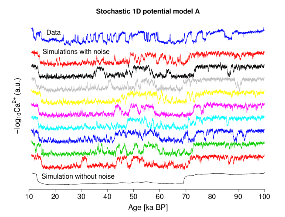
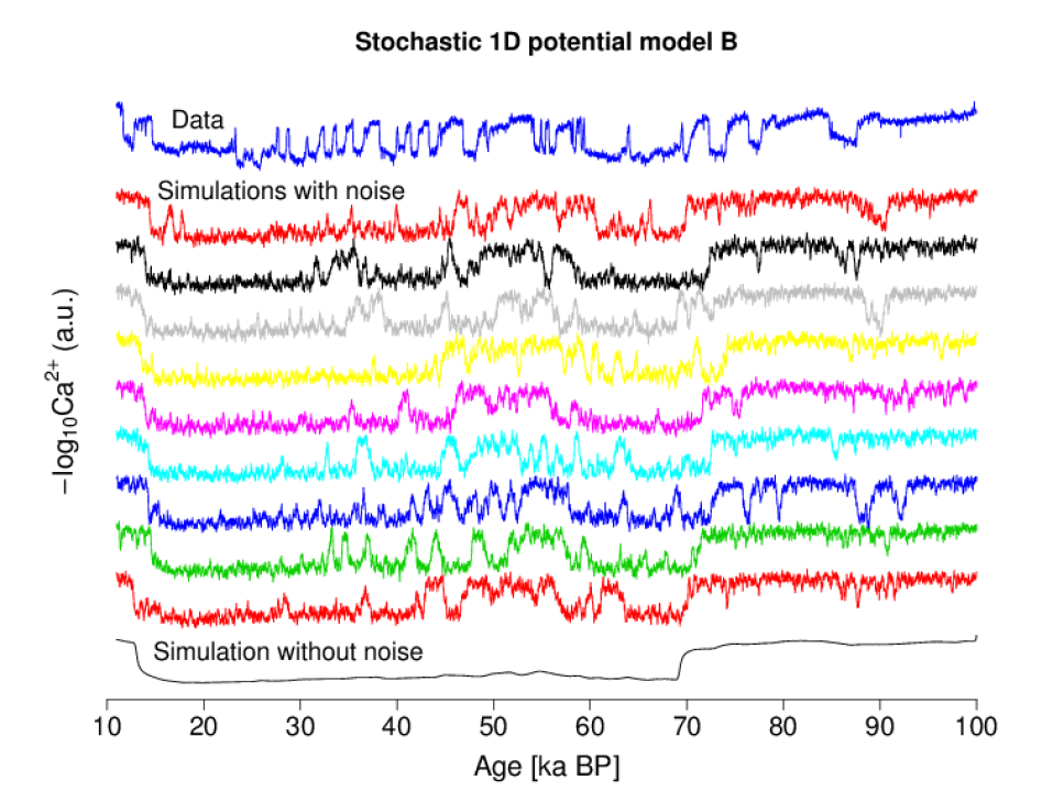
Figure 2: Sample trajectories simulated by the 1D potential model A (top) and model B (bottom) under the full forcing (9 with noise and 1 without noise, i.e., $\sigma=\varepsilon=0$).

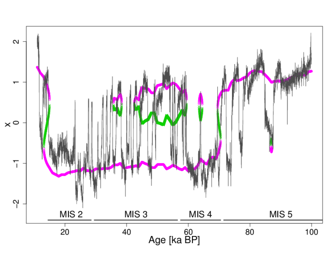
Figure 3: Locations of the local minima (magenta, circle) and the local maximum (green, cross) of the effective potential $U_{\text{eff}}(x,t)$ with respect to $x$. The case of the 1D potential model A with full forcing (see Table 1 for the parameters). Roughly speaking, the state $x(t)$ is stable near the local minima and unstable near the local maximum. The observational data $y$ is represented by a line.

Table 1: Maximum likelihood estimate for the 1D potential model A (the NGRIP $-\log_{10}[\text{Ca}^{2+}]$ data). For each parameter, the maximum likelihood estimator is shown with the standard error.

1D model A	$a_{1}$	$a_{2}$	$a_{3}$	$a_{4}$	$\sigma$	$\varepsilon$	$\gamma_{1}$	$\gamma_{2}$	$\ln L$	BIC	AIC	$K$
Full forcing	$0.048\pm 0.306$	$-1.6\pm 0.2$	$0.14\pm 0.09$	$1.0\pm 0.1$	$1.39\pm 0.04$	$0.046\pm 0.009$	$0.72\pm 0.20$	$2.4\pm 0.3$	$719.4$	$-1374.4$	$-1422.8$	8
Insolation only	$0.31\pm 0.29$	$-1.6\pm 0.2$	$0.012\pm 0.089$	$0.83\pm 0.08$	$1.34\pm 0.04$	$0.054\pm 0.007$	$0.75\pm 0.19$	$\equiv 0$	$691.3$	$-1326.2$	$-1368.6$	7
Ice volume only	$-0.081\pm 0.303$	$-1.7\pm 0.2$	$0.15\pm 0.09$	$1.0\pm 0.09$	$1.38\pm 0.03$	$0.048\pm 0.008$	$\equiv 0$	$2.5\pm 0.3$	$712.4$	$-1368.5$	$-1410.8$	7
No forcing	$0.19\pm 0.29$	$-1.7\pm 0.2$	$0.018\pm 0.088$	$0.80\pm 0.08$	$1.33\pm 0.03$	$0.056\pm 0.007$	$\equiv 0$	$\equiv 0$	$683.3$	$-1318.2$	$-1354.6$	6

Table 2: Maximum likelihood estimate for the 1D potential model B (the NGRIP $-\log_{10}[\text{Ca}^{2+}]$ data).

1D model B	$a_{1}$	$a_{2}$	$a_{3}$	$a_{4}$	$\sigma$	$\varepsilon$	$\gamma_{1}$	$\gamma_{2}$	$\ln L$	BIC	AIC	$K$
Full forcing	$0.062\pm 0.325$	$-1.8\pm 0.25$	$0.15\pm 0.10$	$1.2\pm 0.09$	$1.48\pm 0.02$	$\equiv 0$	$0.80\pm 0.21$	$2.7\pm 0.3$	$716.1$	$-1375.8$	$-1416.1$	7
Insolation only	$0.37\pm 0.32$	$-1.9\pm 0.2$	$0.006\pm 0.096$	$0.97\pm 0.08$	$1.46\pm 0.02$	$\equiv 0$	$0.87\pm 0.20$	$\equiv 0$	$684.3$	$-1320.2$	$-1352.4$	6
Ice volume only	$-0.073\pm 0.322$	$-1.9\pm 0.2$	$0.16\pm 0.10$	$1.1\pm 0.09$	$1.47\pm 0.02$	$\equiv 0$	$\equiv 0$	$2.7\pm 0.3$	$708.5$	$-1368.5$	$-1400.9$	6
No forcing	$0.22\pm 0.31$	$-2.0\pm 0.2$	$0.012\pm 0.095$	$0.94\pm 0.08$	$1.46\pm 0.02$	$\equiv 0$	$\equiv 0$	$\equiv 0$	$675.2$	$-1310.1$	$-1334.2$	5

Table 3: Maximum likelihood estimate for the oscillator model A (the NGRIP $-\log_{10}[\text{Ca}^{2+}]$ data).

Oscillator model A	$k$	$x_{*}$	$\alpha$	$\beta$	$\sigma_{1}$	$\sigma_{2}$	$\varepsilon$	$\gamma_{0}$	$\gamma_{1}$	$\gamma_{2}$	$\ln L$	BIC	AIC	$K$
Full forcing	$38\pm 8$	$-0.081\pm 0.017$	$-0.32\pm 2.00$	$58\pm 6$	$1.3\pm 0.1$	$0.78\pm 0.11$	$0.074\pm 0.010$	$-0.15\pm 0.10$	$0.34\pm 0.10$	$0.57\pm 0.14$	$914.8$	$-1748.9$	$-1809.6$	10
Insolation only	$28\pm 6$	$-0.079\pm 0.017$	$-0.17\pm 2.05$	$59\pm 6$	$1.3\pm 0.1$	$1.1\pm 0.2$	$0.073\pm 0.010$	$-0.19\pm 0.14$	$0.48\pm 0.13$	$\equiv 0$	$909.2$	$-1745.9$	$-1800.4$	9
Ice volume only	$33\pm 7$	$-0.080\pm 0.017$	$-0.098\pm 2.067$	$59\pm 6$	$1.3\pm 0.1$	$0.93\pm 0.15$	$0.075\pm 0.010$	$-0.13\pm 0.12$	$\equiv 0$	$0.70\pm 0.16$	$910.0$	$-1747.5$	$-1802.0$	9
No forcing	$22\pm 5$	$-0.078\pm 0.017$	$0.013\pm 2.160$	$60\pm 6$	$1.3\pm 0.1$	$1.4\pm 0.3$	$0.073\pm 0.010$	$-0.16\pm 0.18$	$\equiv 0$	$\equiv 0$	$904.1$	$-1743.7$	$-1792.2$	8

Table 4: Maximum likelihood estimate for the oscillator model B (the NGRIP $-\log_{10}[\text{Ca}^{2+}]$ data).

Oscillator model B	$k$	$x_{*}$	$\alpha$	$\beta$	$\sigma_{2}$	$\varepsilon$	$\gamma_{0}$	$\gamma_{1}$	$\gamma_{2}$	$\ln L$	BIC	AIC	$K$
Full forcing	$100\pm 17$	$-0.052\pm 0.017$	$17\pm 5$	$130\pm 13$	$0.88\pm 0.14$	$0.12\pm 0.003$	$-0.15\pm 0.11$	$0.33\pm 0.11$	$0.57\pm 0.16$	$911.2$	$-1749.9$	$-1804.4$	9
Insolation only	$75\pm 15$	$-0.051\pm 0.017$	$18\pm 5$	$134\pm 14$	$1.2\pm 0.2$	$0.12\pm 0.003$	$-0.19\pm 0.15$	$0.48\pm 0.15$	$\equiv 0$	$906.7$	$-1748.9$	$-1797.4$	8
Ice volume only	$86\pm 16$	$-0.053\pm 0.017$	$17\pm 5$	$131\pm 13$	$1.0\pm 0.2$	$0.12\pm 0.002$	$-0.12\pm 0.13$	$\equiv 0$	$0.70\pm 0.18$	$907.4$	$-1750.4$	$-1798.8$	8
No forcing	$58\pm 13$	$-0.051\pm 0.017$	$18\pm 5$	$136\pm 14$	$1.6\pm 0.3$	$0.12\pm 0.002$	$-0.15\pm 0.20$	$\equiv 0$	$\equiv 0$	$902.5$	$-1748.6$	$-1791.0$	7

Table 5: Maximum likelihood estimate for the 1D potential model (the NGRIP $\delta^{18}$O${}_{\text{ice}}$ data).

$a_{1}$	$a_{2}$	$a_{3}$	$a_{4}$	$\sigma$	$\varepsilon$	$\gamma_{1}$	$\gamma_{2}$	$\ln L$
$0.46\pm 0.35$	$-0.31\pm 0.29$	$0.011\pm 0.099$	$0.55\pm 0.08$	$1.7\pm 0.07$	$0.27\pm 0.007$	$1.2\pm 0.3$	$1.9\pm 0.4$	$-1578.0$

Table 6: Maximum likelihood estimate for the oscillator model A (the NGRIP $\delta^{18}$O${}_{\text{ice}}$ data).

$k$	$x_{*}$	$\alpha$	$\beta$	$\sigma_{1}$	$\sigma_{2}$	$\varepsilon$	$\gamma_{0}$	$\gamma_{1}$	$\gamma_{2}$	$\ln L$
$581\pm 131$	$-0.63\pm 0.06$	$165\pm 28$	$74\pm 14$	$5.7\pm 0.4$	$0.62\pm 0.07$	$10^{-6}$ (lower bound)	$-0.13\pm 0.08$	$0.33\pm 0.08$	$0.61\pm 0.11$	$-1511.4$

3.2 Maximum likelihood estimate for the oscillator model: the case of Ca²⁺ record

The oscillator models A and B with different forcings are calibrated with the 20-year average NGRIP Ca²⁺ record. The oscillator model A has two significant local maxima in the likelihood function $L(\theta)$ (see Supplementary Fig. S1). The MLE of model A is characterized by a small negative value of $\alpha$ and a relatively large value of $\sigma_{1}$ (Table 3). The MLE of model B is characterized by a large positive value of $\alpha$ and $\sigma_{1}=0$ (Table 4). This corresponds to the second local maximum of the model A. Because $k,\,\beta\gg 1$ in both models, Eq. (4) is the fast system, and Eq. (5) is the slow system. Note the slow system parameters $\gamma_{0,1,2}$ and $\sigma_{2}$ have almost the same mean and standard deviation in both models while some of the fast system parameters, $k$, $\alpha$, and $\beta$, are rather different. This suggests that the inference on the external forcings is robust. Based on BIC scores, the models with full forcing or the ice volume forcing are rather preferred to those with insolation forcing or without forcing (in both models A and B). This is also the same if the AIC is used. Figure 4 shows sample trajectories of oscillator model A (top) and B (bottom) under the full forcing, respectively. There seems to be no substantial difference between A and B. Indeed, given that the difference between the lowest BICs is less than 2, it is difficult to select one from A and B.

For better understanding of the dynamics, let us consider the deterministic system obtained by setting $\sigma_{1}=\sigma_{2}=0$ and replacing $\gamma_{1}I(t)-\gamma_{2}V(t)$ by a constant external forcing $F_{\text{ext}}$ in Eqs. (4) and (5). For the model A (with $\hat{\alpha}=-0.32<0$), the deterministic system has a limit cycle if the external forcing is $-0.025<F_{\text{ext}}<0.171$. However, the limit cycle is much smaller than the observed stochastic cycles in the presence of noise, as shown in Fig. 5. The stochastic cycles are formed around the slow manifold of the system, $v=\{\alpha x+\frac{\beta}{3}[(x-x_{*})^{3}+x_{*}^{3}]\}/k$, away from the limit cycle. Hence, they are termed noise-induced oscillations. This result is consistent with the result obtained by Kwasniok (2013) for the unforced case. For the model A, the sign of parameter $\alpha$ is actually uncertain because of the large standard error ($2.0$), but noise-induced oscillations appear regardless of the sign of $\alpha$. For the model B ($\hat{\alpha}>0$), the deterministic system never exhibits self-sustained oscillations, but the system can exhibit noise-induced oscillations.

The time scale of noise-induced oscillations emerges from the interplay between the underlying deterministic system and the system noise. Figure 6 shows the average period between successive warming transitions as a function of the constant external forcing $F_{\text{ext}}$ (for the case of model A), where a warming transition is defined as in Section 1. The U-shape dependency of the period is similar to that of deep-decoupling oscillation models (Winton, 1993; Schulz, 2002b; Colin de Verdière, 2007), where the freshwater flux is the control parameter. Using a deep-decoupling model forced by freshwater flux proportional to a reconstructed ice volume, Sima et al (2004) argue that the Younger Dryas event may be an intrinsic feature associated with deglaciations, and it seems to be not an accident but an inevitable one. In our ensemble simulations in Fig. 4, the occurrence of Younger Dryas-type event depends on the realization of system noise.

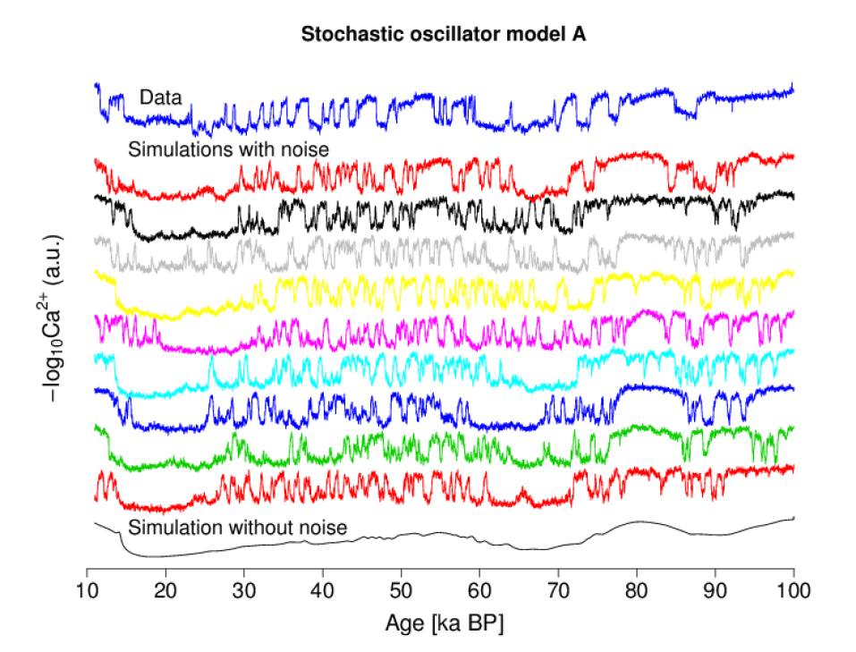
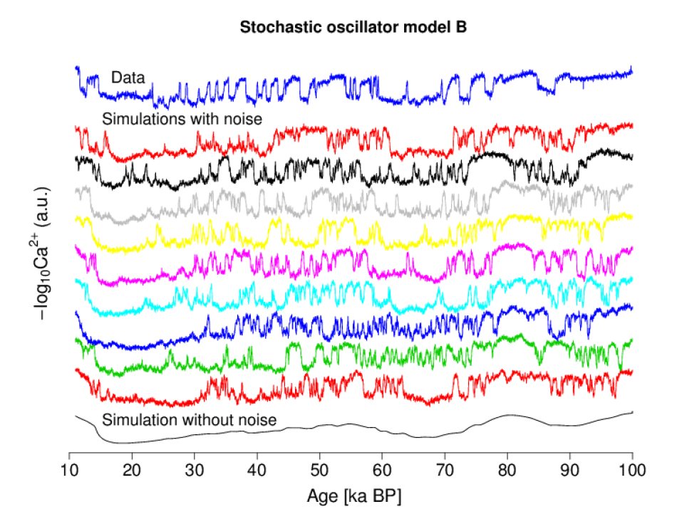
Figure 4: Sample trajectories simulated by the oscillator model A (top) and model B (bottom) under the full forcing (9 with noise and 1 without noise, i.e., $\sigma_{1}=\sigma_{2}=\varepsilon=0$).

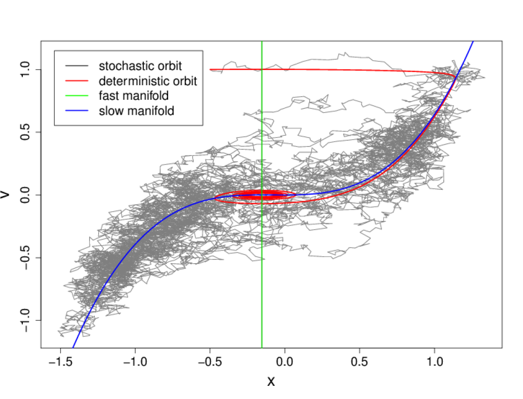
Figure 5: A sample trajectory of the oscillator model A of Eqs. (4) and (5) for $\gamma_{1}=\gamma_{2}=0$ (gray). The red curve is a trajectory approaching the limit cycle for the deterministic system for $\sigma_{1}=\sigma_{2}=0$ and $\gamma_{1}=\gamma_{2}=0$. The other parameters are set to the maximum likelihood estimator in Table 3 (the full forcing case).

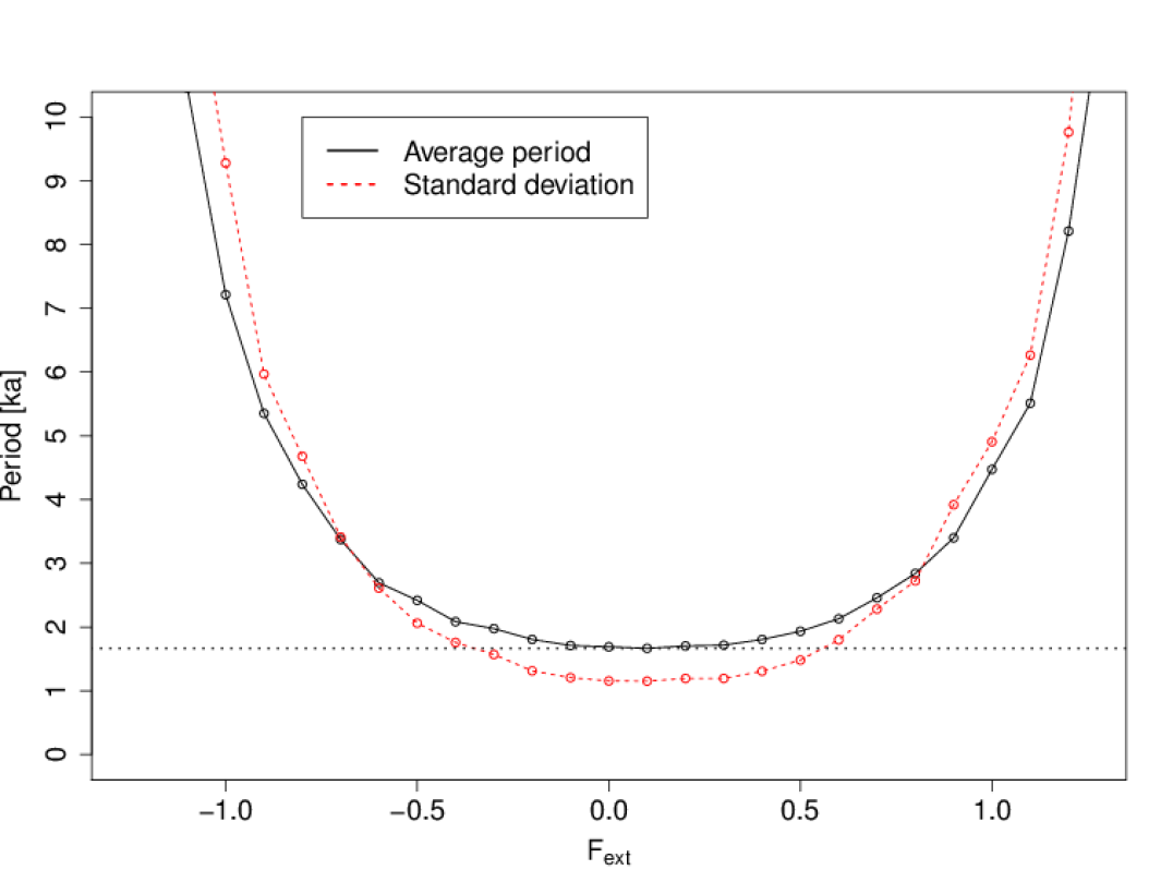
Figure 6: The average period (black, solid) and its standard deviation (red, dashed) between successive warming transitions simulated by stochastic oscillator model A. They are presented as functions of the constant external forcing $F_{\text{ext}}$. See Section 1 for the definition of a warming transition. The average period takes the minimum $\sim$1665 year at $F_{\text{ext}}\approx 0.1$. The parameters are set to the maximum likelihood estimator in Table 3 (the full forcing case).

3.3 Maximum likelihood estimate: the case of $\delta^{18}$O${}_{\text{ice}}$ record

The 1D potential model A and the oscillator model A are calibrated on the 20-year average NGRIP $\delta^{18}$O${}_{\text{ice}}$ record (Rasmussen et al, 2014) to assess proxy dependence. As shown in Tables 1–6, the values of forcing parameters $\gamma_{1,2}$ are consistent between Ca²⁺ and $\delta^{18}$O${}_{\text{ice}}$, but the other parameters are rather different. On the other hand, the values of maximum log-likelihood for $\delta^{18}$O${}_{\text{ice}}$ ($-1578.0$ and $-1511.4$) are significantly lower than those for Ca²⁺ ($719.4$ and $914.8$). This may be taken as an informal indicator that the fit on $\delta^{18}$O${}_{\text{ice}}$ is poorer than on Ca²⁺. Therefore, in this study, we discuss the influence of external forcings based on the models calibrated on Ca²⁺.

4 Model comparisons

The models calibrated in the previous Section are compared using several criteria. The probability density is a useful criterion for assessing stochastic dynamical systems models, but here all models reproduce the probability density of the record relatively well. Hence, it is only discussed in the Supplementary Fig. S2.

4.1 Sample autocorrelation function

First, we assess the model performance by the sample autocorrelation function (ACF) as in Kwasniok and Lohmann (2009). Figure (7) shows the sample ACF of the 20-year average NGRIP Ca²⁺ data (solid line) and the ensemble mean of the sample ACF simulated by each model (inner dashed line). The outer dashed lines present $\pm 1$ s.d. The sample ACF of the data is explained well by the oscillator models with the full forcing and relatively well by the oscillator models with the ice volume forcing. The difference between the model A and B is negligible.

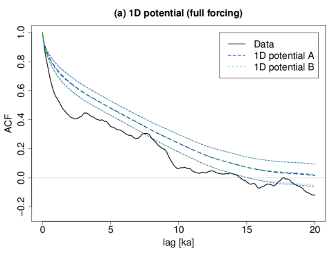
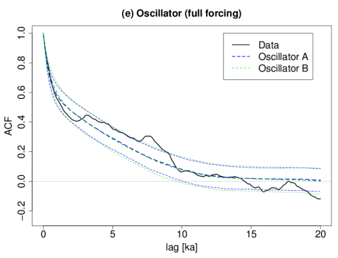
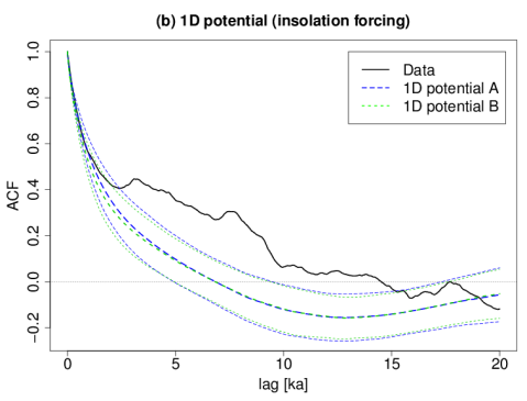
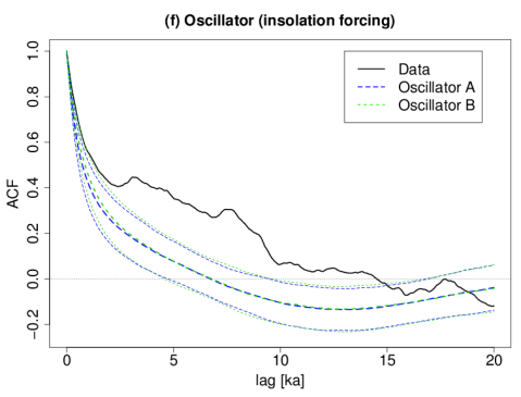
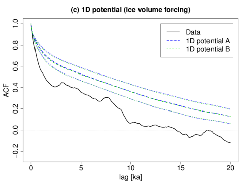
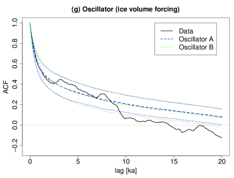
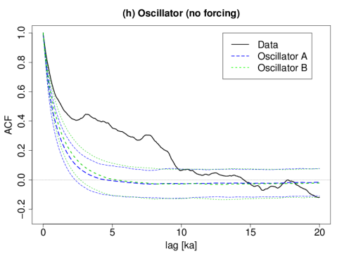
Figure 7: Sample autocorrelation function (ACF) of the 20-year average NGRIP Ca²⁺ data (solid line) and the ensemble mean of the sample ACF of each model (inner dashed line). The outer dashed lines show $\pm 1$ s.d. All sample ACFs are calculated over 11–100 ka BP. Initial conditions are randomly taken at $100$ ka BP from a normal distribution $p(x)=\mathcal{N}(1,1)$ for the 1D potential model, and from $p(x)=\mathcal{N}(1,1)$ and $p(v)=\mathcal{N}(1,1)$ for the stochastic oscillator models. The ensemble size is $10^{3}$ for all the models. The ensemble mean of the sample ACFs does not converge to zero even in the stationary cases (d) and (h) because of the finite sample length effect (Trenberth, 1984).

4.2 Model comparison based on the occurrence frequency of warming transitions

We calculate the average number of warming transitions $\langle n(t)\rangle$ for each 20-ka window [$t-10$ ka, $t+10$ ka] for each model, where $\langle\cdot\rangle$ means the ensemble average for $10^{3}$ simulations with different noise realizations and initial conditions. The same definition for a warming transition is used as in the Introduction. Figures 8 and 9 show the number of warming transitions $n(t)$ for the NGRIP Ca²⁺ data (red) and the average number of warming transitions $\langle n(t)\rangle$ for each model (blue), where the shaded error bar represents $\pm 1$ s.d. As mentioned in the Introduction, the number of warming transitions $n(t)$ in the observed record increased from MIS4 to MIS3 and decreased from MIS3 to MIS2. These frequency changes are well reproduced by the oscillator model A with full forcing (Fig. 9(a)) or with only ice volume forcing (Fig. 9(c)). The performance of oscillator model B is similar to that of oscillator model A, but the frequency $n(t)$ is larger by about one. These results are robust against small changes of the thresholds ($\pm 0.2$ with respect to $y$).

However, the stochastic oscillator models fail to produce the low values of $n(t)$ in late MIS 5 ($70$–$90$ ka BP), while this low frequency is somewhat captured by the stochastic 1D potential models with full forcing (Fig. 8(a)) or with only ice volume forcing (Fig. 8(c)).

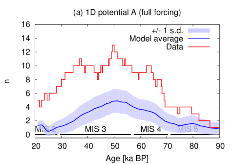
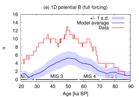
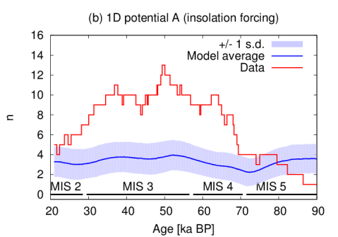
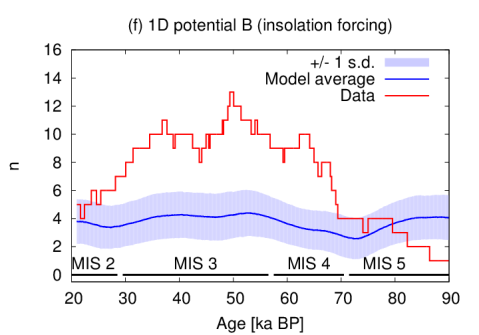
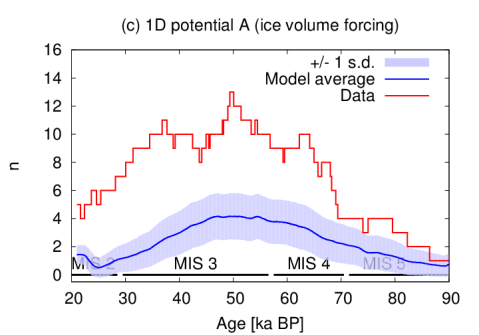
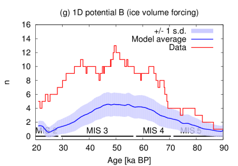
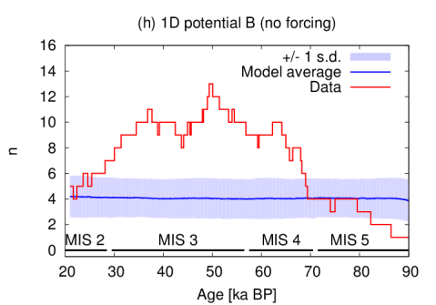
Figure 8: The number of warming transitions $n(t)$ for each 20-ka window [$t-10$ ka, $t+10$ ka]. See text for the definition of a warming transition. The red curve is $n(t)$ of the 20-year average NGRIP Ca²⁺ data, and the blue curve is the ensemble mean $\langle n(t)\rangle$ simulated by each 1D potential model with different noise realizations. The shaded error bar represents $\pm 1$ s.d. Initial conditions are randomly taken at $100$ ka BP from a normal distribution $p(x)=\mathcal{N}(1,1)$. The ensemble size is $10^{3}$ for all the models.

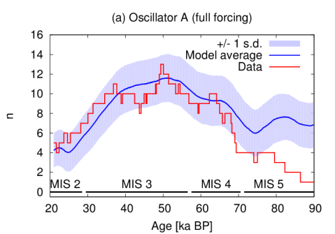
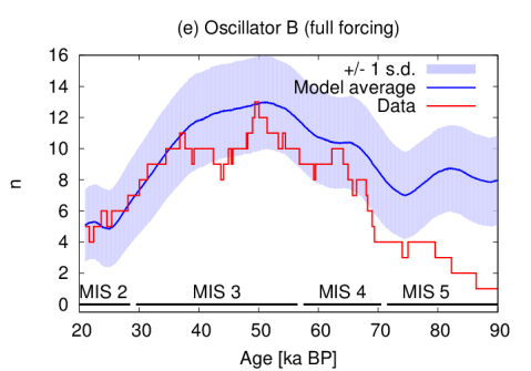
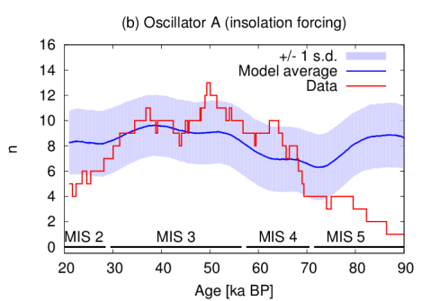
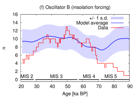
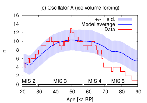
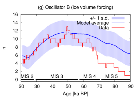
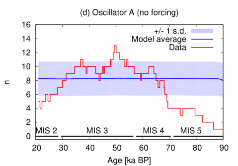
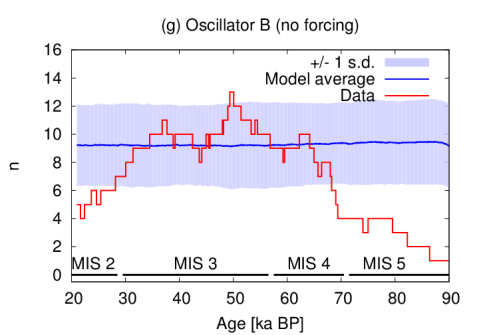
Figure 9: The number of warming transitions $n(t)$ for each 20-ka window [$t-10$ ka, $t+10$ ka]. See text for the definition of a warming transition. The red curve is $n(t)$ of the 20-year average NGRIP Ca²⁺ data, and the blue curve is the ensemble mean $\langle n(t)\rangle$ simulated by each oscillator model with different noise realizations. The shaded error bar represents $\pm 1$ s.d. Initial conditions are randomly taken at $100$ ka BP from normal distributions $p(x)=\mathcal{N}(1,1)$ and $p(v)=\mathcal{N}(1,1)$. The ensemble size is $10^{3}$ for all the models.

4.3 BIC and the BIC difference

1D potential model vs. oscillator model. The lowest BIC of the 1D potential model for four different forcing scenarios is $-1375.8$ (Table 2) and the highest BIC of the oscillator models is $-1743.7$ (Table 3). Thus, the BIC difference between the worst stochastic oscillator model and the best stochastic 1D potential model is $367.9$. This is very strong evidence in favor of the oscillator models against the 1D potential models. Note that Kwasniok (2013) also reports strong evidence in favor of the oscillator model against the 1D potential model for the unforced case $\gamma_{i}=0$ ($i=0,1,2$) ($\Delta$BIC$=12.9$ for GRIP $\delta^{18}$O${}_{\text{ice}}$ and $\Delta$BIC$=14.6$ for NGRIP $\delta^{18}$O${}_{\text{ice}}$).

Comparison between different forcings. As already shown in Tables 1–4, the BIC scores suggest that the full forcing or the ice volume forcing are more supported than the insolation forcing or the null forcing. This is consistent with the results obtained by using the sample ACF and the frequency of warming transitions. However, the strength of evidence in favor of a particular forcing depends on the model class as shown in Tables 7–10. The evidence in favor of the ice volume forcing against the insolation forcing ($\Delta$BIC) is very strong for the 1D potential models (42.3 for A and 48.4 for B), but it is weak for the oscillator models (1.56 for A and 1.43 for B). On the other hand, the examination of the ACF and the occurrence frequency of warming transitions suggest qualitatively a more important role for the ice volume forcing than for the insolation forcing.

Table 7: BIC difference $\Delta\text{BIC}_{ij}=\text{BIC}_{j}-\text{BIC}_{i}$ as evidence in favor of a model $i$ (row) against a model $j$ (column): the case of the stochastic 1D potential model A. The asterisk means the minus value of corresponding diagonal element.

	vs. Full forcing	vs. Insolation only	vs. Ice volume only	vs. No forcing
Full forcing	$0$	$48.3$ (very strong)	$5.96$ (positive)	$56.2$ (very strong)
Insolation only	$\ast$	$0$	$\ast$	$7.98$ (strong)
Ice volume only	$\ast$	$42.3$ (very strong)	$0$	$50.3$ (very strong)
No forcing	$\ast$	$\ast$	$\ast$	$0$

Table 8: BIC difference $\Delta\text{BIC}_{ij}=\text{BIC}_{j}-\text{BIC}_{i}$ as evidence in favor of a model $i$ (row) against a model $j$ (column): the case of the stochastic 1D potential model B. The asterisk means the minus value of corresponding diagonal element.

	vs. Full forcing	vs. Insolation only	vs. Ice volume only	vs. No forcing
Full forcing	$0$	$55.6$ (very strong)	$7.18$ (positive)	$65.7$ (very strong)
Insolation only	$\ast$	$0$	$\ast$	$10.1$ (very strong)
Ice volume only	$\ast$	$48.4$ (very strong)	$0$	$58.5$ (very strong)
No forcing	$\ast$	$\ast$	$\ast$	$0$

Table 9: BIC difference $\Delta\text{BIC}_{ij}=\text{BIC}_{j}-\text{BIC}_{i}$ as evidence in favor of a model $i$ (row) against a model $j$ (column): the case of the stochastic oscillator model A. The asterisk means the minus value of corresponding diagonal element.

	vs. Full forcing	vs. Insolation only	vs. Ice volume only	vs. No forcing
Full forcing	$0$	$3.02$ (positive)	$1.46$ (weak)	$5.28$ (positive)
Insolation only	$\ast$	$0$	$\ast$	$2.26$ (positive)
Ice volume only	$\ast$	$1.56$ (weak)	$0$	$3.83$ (positive)
No forcing	$\ast$	$\ast$	$\ast$	$0$

Table 10: BIC difference $\Delta\text{BIC}_{ij}=\text{BIC}_{j}-\text{BIC}_{i}$ as evidence in favor of a model $i$ (row) against a model $j$ (column): the case of the stochastic oscillator model B. The asterisk means the minus value of corresponding diagonal element.

	vs. Full forcing	vs. Insolation only	vs. Ice volume only	vs. No forcing
Full forcing	$0$	$0.97$ (weak)	$\ast$	$1.32$ (weak)
Insolation only	$\ast$	$0$	$\ast$	$0.36$ (weak)
Ice volume only	$0.47$ (weak)	$1.43$ (weak)	$0$	$1.79$ (weak)
No forcing	$\ast$	$\ast$	$\ast$	$0$

5 Implication

The stochastic oscillator model A with full forcing could estimate the occurrence frequency of DO events in the last glacial period (MISs 2–4) though it could not in the early glaciation stage MIS 5. Hence we assume that the model can be extended to past few glacial periods with enough ice sheets, and we predict the frequency of abrupt millennial-scale climate changes in the last four glacial periods under this assumption.

It is difficult to use Greenland ice core records to infer the frequency of abrupt climate changes before the Eemian interglacial because they are disturbed in chronology due to ice-folding near the bedrock. However, the information may be inferred from Iberian margin SST records derived from the U${}^{k^{\prime}}_{37}$ alkenone index. A U${}^{k^{\prime}}_{37}$-SST record in a composite of cores MD01-2444 and MD01-2443 over the past four glacial cycles is shown in Fig. 10, which is reproduced based on Martrat et al (2007). Similar SST variations are observed also in another Iberian margin core (ODP-997A, not shown here) (Martrat et al, 2004). These U${}^{k^{\prime}}_{37}$-SST records show warmings and coolings corresponding to major DO events in Greenland ice cores.

Martrat et al (2007) identified cold and warm climate events in the U${}^{k^{\prime}}_{37}$-SST record and labelled them as Iberian margin stadials (IMSs) and Iberian margin interstadials (IMIs), respectively. For example, 2IMI-3 denotes the third interstadial within the second glacial cycle (see Fig. 10). We use this identification of events to estimate the frequency of abrupt millennial-scale climate changes in the North Atlantic region though the labels were originally introduced by Martrat et al (2007) for the purpose of discussion. The timing of each warming transition is set at the time of the largest increase of SST between each IMS and subsequent IMI.

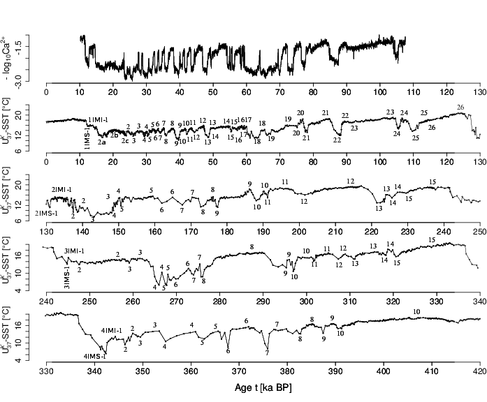
Figure 10: Top panel shows the 20-year average NGRIP Ca²⁺ concentration (Rasmussen et al, 2014). The other panels show the U${}^{k^{\prime}}_{37}$–SST in a composite of cores MD01-2444 and MD01-2443 reproduced based on Martrat et al (2007). The stage numbers of the Iberian Margin Interstadials (IMI) are shown above the line, and those of the Iberian Margin Stadials (IMS) are shown below the line.

Figures 11(a-ii), (b-ii), (c-ii), and (d-ii) show the number of warming transitions $n(t)$ estimated from the Iberian margin SST (magenta) and the average number of warming transitions $\langle n(t)\rangle$ simulated by the stochastic oscillator model (blue). Both are roughly correlated though a phase lag is identified in MIS 8. However, peak levels largely differ between the simulations and the data. We may guess two reasons for the difference: one reason may be that some events do not clearly appear in the SST record. Indeed, some events in Iberian margin SST records seem difficult to be identified without information from Greenland ice cores (for example, 1IMS-14 and 1IMI-13, and 1IMS-23 and 1IMI-22). Another reason may be that some rapid events are missed in the SST record due to its low time resolution especially in the older part. Figures 11(a-iii), (b-iii), (c-iii), and (d-iii) (green line) show the average number of warming transitions $\langle n(t)\rangle$ for the simulated time series whose values are sampled at the same time points as the SST record. The number of warming transitions is then similar to that seen in SST data. We therefore suggest that the number of the abrupt climate changes in the past glacial periods was more frequent than that seen in the SST data by Martrat et al (2007).

We now further examine two previous observations. First, Martrat et al (2004) observed the higher number of abrupt events during MISs 2–4 compared to MIS 6. Consistently, the model simulates a higher average number of warming transitions $\langle n(t)\rangle$ during MISs 2–4 compared to MIS 6 though the difference is smaller in the simulation than in the observation. Recall Fig. 6, which shows that stochastic oscillations are frequent when the external forcing $F_{\text{ext}}(t)=\gamma_{1}I(t)-\gamma_{2}V(t)$ is in an intermediate range. Specifically, the average period of oscillations is less than 2000 years for $-0.3<F_{\text{ext}}<0.5$. As shown in Figs. 11(a-i) and (b-i), the external forcing $F_{\text{ext}}(t)$ is in the intermediate range for short times in MIS 6 but for a long time in MISs 2–4. This explains why the number of warming transitions $n(t)$ during MISs 2–4 is higher than during MIS 6.

Secondly, Martrat et al (2007) consider that the millennial-scale climate changes become abundant as the Pleistocene progresses to the present. However, if the model can be extended to the older glacial periods, millennial-scale climate changes in MIS 8 and MIS 10 are expected to be as frequent as in the last glacial period, as shown in Figs. 11(c-ii) and (d-ii).

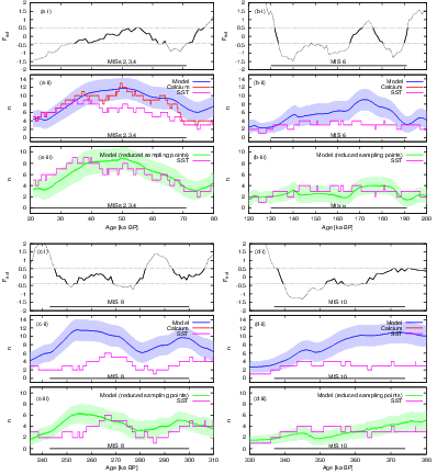
Figure 11: Simulations of abrupt millennial-scale climate changes in the past four glacial periods (a) MISs 2–4, (b) MIS 6, (c) MIS 8, and (d) MIS 10. (i) Variations of the external forcing $F_{\text{ext}}(t)=\gamma_{1}I(t)-\gamma_{2}V(t)$. Thick parts of the line highlight the range with active stochastic oscillations, $-0.3<F_{\text{ext}}<0.5$, where the average period between successive warming transitions is less than 2000 years. (ii) The number of warming transitions $n(t)$ for each 20-ka window [$t-10$ ka, $t+10$ ka]. The red curve is $n(t)$ for the 20-year average NGRIP Ca²⁺ data. The magenta line is $n(t)$ for the Iberian margin U${}^{\text{k'}}_{37}$-SST of a composite of cores MD01-2444 and MD01-2443 (Martrat et al, 2007), and the blue curve is the ensemble mean $\langle n(t)\rangle$ simulated by the fully-forced stochastic oscillator model A with different noise realizations. The shaded error bar represents $\pm 1$ s.d. (iii) The green curve is the ensemble mean $\langle n(t)\rangle$ for the simulated time series whose values are sampled at the same time points as the SST recored. Initial conditions are randomly taken at $t=420$ ka BP from normal distributions $p(x)=\mathcal{N}(1,1)$ and $p(v)=\mathcal{N}(1,1)$.

6 Conclusion

The influence of external forcings on DO events was investigated with statistical modeling based on simple stochastic dynamical systems: the 1D potential model and the oscillator model forced by the northern hemisphere summer insolation change and the global ice volume change. We estimated model parameters by maximizing the likelihood with the NGRIP Ca²⁺ record. The stochastic oscillator model at least with the ice volume forcing reproduces well the sample autocorrelation function of the record and the frequency changes of warming transitions in the last glacial period across MISs 2–4. The model performance is improved with the additional insolation forcing. The BIC scores also suggest that the ice volume forcing is relatively more important than the insolation forcing, though the strength of evidence ($\Delta$BIC) depends on the model assumption on the system and noise.

It is worth mentioning that not only the influence of the insolation forcing but also the influence of the ice volume forcing is detected in grain-size records from the Chinese Loess Plateau (a proxy for the East Asian winter monsoon intensity) by spectral analyses (Ding et al, 1995; Li et al, 2015). This is consistent with our result, given the proximity of the sources of Chinese loess archives and the sources of terrestrial dusts found in Greenland.

Finally, using the fully-forced oscillator model A calibrated in the last glacial cycle, we simulated the average number of warming transitions $\langle n(t)\rangle$ for each 20-ka moving window over the past four glacial periods, and compared the result with an Iberian margin SST data (Martrat et al, 2007). The simulation result supports the previous observation by Martrat et al (2004) that abrupt millennial-scale climate changes in the penultimate glacial (MIS 6) is less frequent than in the last glacial (MISs 2–4). On the other hand, it suggests that the number of abrupt millennial-scale climate changes in older glacial periods (MISs 6, 8, and 10) might be larger than inferred from the SST data. If the model can be extended to the older glacial periods, the millennial-scale climate changes in MIS 8 and MIS 10 are expected to be as frequent as in the last glacial period.

The LR04 record, used here as a proxy for the global ice volume, contains information about astronomical insolation forcing. Hence, the ice volume forcing implicitly includes a component of the insolation forcing. It is therefore not so surprising to find only weak evidence for the need of additional insolation forcing. We should be cautious not to interpret our result as evidence that the global ice volume is the only physical factor controlling the frequency changes of DO events.

The calibrated models did not reproduce well the low occurrence frequency of DO events in the last glaciation period (MIS 5) (Fig. 9). A use of another ice volume estimate (Bintanja et al, 2005) modifies the discrepancy slightly but not substantially (data not shown). To overcome this, we would need to examine the model assumptions introduced for simplicity. The orography of ice sheets might be more effective than the global ice volume (Zhang et al, 2014). Multiplicative effects of the insolation and the ice volume might be important, given the ice-albedo feedback. A state-dependent noise may have to be considered (Ditlevsen, 1999; Timmermann and Lohmann, 2000). Indeed, fluctuations in $\delta^{18}$O${}_{\text{ice}}$ have larger variances in stadial than in interstadial (Ditlevsen et al, 2002). Non-Gaussian noise and/or temporally-correlated noise might also be suitable to represent external disturbances (such as massive iceberg discharges) (Ditlevsen, 1999).