NRCPS-HE-45-2015

Spectrum and Entropy of C-systems

MIXMAX Random Number Generator

Konstantin Savvidy^@ and George Savvidy^∗

^∗Institute of Nuclear and Particle Physics

Demokritos National Research Center, Ag. Paraskevi, Athens, Greece

^@ College of Science, Nanjing University of Aeronautics and Astronautics

Nanjing 211106, China.

Abstract

The uniformly hyperbolic Anosov C-systems defined on a torus have very strong instability of their trajectories, as strong as it can be in principle. These systems have exponential instability of all their trajectories and as such have mixing of all orders, nonzero Kolmogorov entropy and a countable set of everywhere dense periodic trajectories. In this paper we are studying the properties of their spectrum and of the entropy. For a two-parameter family of C-system operators $A(N,s)$, parametrised by the integers $N$ and $s$, we found the universal limiting form of the spectrum, the dependence of entropy on $N$ and the period of its trajectories on a rational sublattice. One can deduce from this result that the entropy and the periods are sharply increasing with $N$. We present a new three-parameter family of C-operators $A(N,s,m)$ and analyse the dependence of its spectrum and of the entropy on the parameter $m$. We are developing our earlier suggestion to use these tuneable Anosov C-systems for multipurpose Monte-Carlo simulations. The MIXMAX family of random number generators based on Anosov C-systems provide high quality statistical properties, thanks to their large entropy, have the best combination of speed, reasonable size of the state, tuneable parameters and availability for implementing the parallelisation.

1 Introduction

The uniformly hyperbolic Anosov C-systems defined on a torus have very strong instability of their trajectories, as strong as it can be in principle [1]. These systems have exponential instability of all their trajectories and as such have mixing of all orders, nonzero Kolmogorov entropy and a countable set of everywhere dense periodic trajectories. In this paper we are studying the properties of their spectrum and of their entropy and are developing our earlier suggestion to use the Anosov C-systems for Monte-Carlo simulations [2].

The particular system chosen for investigation is the one realising linear automorphisms of the unit hypercube in Euclidean space $\mathbb{R}^{N}$ with coordinates $(u_{1},...,u_{N})$[1, 2, 3, 4]:

$$u_{i}^{(k+1)}=\sum_{j=1}^{N}A_{ij}\,u_{j}^{(k)}~{}~{}~{}~{}~{}\textrm{mod}~{}1,~{}~{}~{}~{}~{}~{}~{}~{}~{}k=0,1,2,...$$ (1.1)

where the components of the vector $u^{(k)}$ are defined as

$$u^{(k)}=(u^{(k)}_{1},...,u^{(k)}_{N}).$$

The dynamical system defined here by the integer matrix $A$ should have a determinant equal to one $\mathop{\rm Det}A=1$. In order for the automorphisms (1.1) to fulfill the Anosov hyperbolicity C-condition it is necessary and sufficient that the matrix $A$ has no eigenvalues on the unit circle [1]. Therefore the spectrum $\{\Lambda={\lambda_{1}},...,\lambda_{N}\}$ of the matrix $A$ should fulfill the following two conditions:

$$1)~{}\mathop{\rm Det}A={\lambda_{1}}\,{\lambda_{2}}...{\lambda_{N}}=1,~{}~{}~{}~{}~{}2)~{}~{}|{\lambda_{i}}|\neq 1,~{}~{}~{}\forall~{}~{}i.~{}~{}~{}~{}~{}~{}$$ (1.2)

Because the determinant of the matrix $A$ is equal to one, the Liouville’s measure $d\mu=du_{1}...du_{N}$ is invariant under the action of $A$. The inverse matrix $A^{-1}$ is also an integer matrix because $\mathop{\rm Det}A=1$. Therefore $A$ is an automorphism of the unit hypercube onto itself. The conditions (1.2) on the eigenvalues of the matrix $A$ are sufficient to prove that the system represents an Anosov C-system [1] and therefore as such it also represents a Kolmogorov K-system [8, 9, 10, 11, 12] with mixing of all orders and of nonzero entropy.

The eigenvalues of the matrix $A$ can always be sorted by increasing absolute value and divided into the two sets $\{\lambda_{\alpha}\}$ and $\{\lambda_{\beta}\}$ with modulus smaller and larger than one:

$$0<|\lambda_{\alpha}|<1 \textrm{ for }\alpha=1...d$$

$$1<|\lambda_{\beta}|<\infty \textrm{ for }\beta=d{+}1...N.$$ (1.3)

There exist two hyperplanes $X=\{X_{\alpha}\}$ and $Y=\{Y_{\beta}\}$ which are spanned by the corresponding eigenvectors $\{e_{\alpha}\}$ and $\{e_{\beta}\}$ . These invariant planes of the matrix $A$, for which the eigenvalues are outside and inside of the unit circle respectively, define the expanding and contracting invariant spaces, so that the phase trajectories of the dynamical system (1.1) are expanding and contracting under the transformation $A$ at an exponential rate (see Fig.1). The same is true for the inverse evolution which is defined by the matrix $A^{-1}$. For the inverse evolution the contracting and expanding invariant spaces alternate their role.

Figure 1: The eigenvectors of the matrix $A$ $\{e_{\alpha}\}$ and $\{e_{\beta}\}$ define two families of parallel planes $\{X_{\alpha}\}$ and $\{Y_{\beta}\}$ which are invariant under the automorphisms $A$. The automorphism $A$ is contracting the distances between points on the planes belonging to the set $\{X_{\alpha}\}$ and expanding the distances between points on the planes belonging to the set $\{Y_{\beta}\}$. The a) depicts the parallel planes of the sets $\{X_{\alpha}\}$ and $\{Y_{\beta}\}$ and b) depicts their positions after the action of the automorphism $A$.

The exceptional property of the C-system (1.1) is that it has nonzero entropy and that it is possible to calculate its value $h(A)$ in terms of the eigenvalues of the operator $A$. The most convenient way to find out the entropy is to integrate over the whole phase space the logarithm of the volume expansion rate $\lambda(u)$ of an infinitesimal cube which is embedded into the expanding foliation [1, 10, 12, 13, 14, 4]. For the automorphisms (1.1) the coefficient $\lambda(u)$ does not depend on the phase space coordinates $u$ and is equal to the product of eigenvalues $\{\lambda_{\beta}\}$ with modulus larger than one $\lambda(u)=\prod_{\beta}\lambda_{\beta}$, as it was defined in (1). Thus for the Anosov automorphisms (1.1) one can calculate the entropy, which is equal to the sum:

$$h(A)=\sum_{\beta}\ln|\lambda_{\beta}|.$$ (1.4)

This allows to characterise and compare the chaotic properties of different dynamical systems quantitatively by computing and comparing their entropies. As it is obvious from the above formula for the entropy its value depends on the spectral properties of the evolution operator $A$. Also the variety and richness of the periodic trajectories of the C-systems essentially depend on the entropy [1, 4, 17, 18]. Indeed, the number of periodic trajectories $\pi(q)$ of a period $q$ has the form

$$\pi(q)\sim e^{q\ h(A)}/q$$ (1.5)

and tells that a system with larger entropy $h(A)$ is more densely populated by the periodic trajectories of the period $q$. Our aim is to study these characteristics of the C-systems and develop our earlier suggestion to use the Anosov C-systems for Monte-Carlo simulations [3, 4, 15, 16].

The earlier publications concerning the application of the modern results of the ergodic theory to concrete physical systems can be found in [2, 5, 6, 7]. These articles contain review material as well. The recent review articles on random numbers generators for the Monte-Carlo simulations can be found in [24, 25].

In this article we shall explore a two- and three-parameter family of matrix C-operators $A(N,s)$ and $A(N,s,m)$ by calculating their spectrum and the corresponding entropies. This provides us with the knowledge of the behaviour of the entropy as a function of these parameters and allows to classify these dynamical systems by the increase of their chaotic-stochastic properties. The presence of trajectories of a large period is also associated with the value of the entropy of a dynamical system and we shall study the periods of the above C-system trajectories. In the second section we shall study all these properties for the two-parameter family of operators $A(N,s)$. In the third section the tree-parameter family of operators $A(N,s,m)$ will be investigated. In the fourth section we shall consider the application of these systems to generating random numbers for the Monte-Carlo simulations and other multidisciplinary purposes.

2 Two-parameters Family of C-operators $A(N,s)$

We shall start with the two-parameter family of operators introduced in [3], which are parametrised by the integers $N$ and $s$. We are interested in investigating the general properties of the spectrum and the corresponding value of the Kolmogorov entropy. The matrix is of the size $N\times N$, its entries are all integers $A_{ij}\in\mathbb{Z}$, and it has the following form [3]:

$$A(N,s)=\begin{pmatrix}1&1&1&1&...&1&1\\ 1&2&1&1&...&1&1\\ 1&3{+}s&2&1&...&1&1\\ 1&4&3&2&...&1&1\\ &&&...&&&\\ 1&N&N{-}1&~{}N{-}2&...&3&2\end{pmatrix}$$ (2.6)

The operator is constructed so that its entries are increasing together with the size $N$ of the operator, and we have a family of operators which are parametrised by the integers $N$ and $s$. For any integer values of the parameters $N$ and $s$ of the operator $A(N,s)$, if the condition (1.2) is fulfilled, then the operator $A(N,s)$ represents a C-system [2]. In reference [3] and in our Tables 1 and 2, some values of $N$ and $s$ were found for which the C-condition (1.2) is fulfilled. As we mentioned above, the chaotic properties of the C-system operators are quantified through their spectral distributions, the value of the Kolmogorov entropy (1.4) and periodic trajectories on a rational sublattice [2, 3, 4]. The data in the Tables 1, 2 demonstrates that the entropy of the operator $A(N,s)$ strongly depends on $N$ and $s$ and therefore their chaotic-stochastic properties [3] .

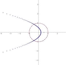
Figure 2: On the left is the distribution of the eigenvalues of the operator $A(N,s)$ and on the right of its inverse operator $A^{-1}(N,s)$ for the $N=256$ and $s=-1$. The unit circle is depicted to separate the eigenvalues inside and outside the circle in accordance with the formula (1). The spectrum of the operators $A(N,s)$ and $A^{-1}(N,s)$ has two real eigenvalues for even $N$, all the rest of the eigenvalues are complex. The minimal $\lambda_{min}\approx 0.25$ and the maximal $\lambda_{max}\approx 3002$ eigenvalues are real. The graph on the left shows only the small eigenvalues which are well approximated by formula (2.8), the large eigenvalues are not depicted. The spectrum of the inverse operator is compact and all eigenvalues can be seen on the right figure. As $N$ tends to infinity $N\rightarrow\infty$, the scale and the shape of the complex curves remain intact, instead, the eigenvalues are filling these curves more and more densely. The value $1/\lambda_{max}$ tends to zero and so lies at the stem of the leaf in the figure on the right.

Size	Magic	Entropy	Log of the period $q$
N	$s$		$\approx\log_{10}(q)$
256	$-1$	$164.5$	${4682}$
256	487013230256099064	193.6	4682

Table 1: Properties of operators $A(N,s$) for large special $s$. The first line is given for comparison, in order to illustrate the improvement of the entropy of the generator for the large $s$ (in the second line). The period $q$ is defined in (2.10), (4.15).

Size	Magic	Entropy	Log of the period q
N	$s$		$\approx\log_{10}(q)$
7307	0	4676.5	134158
20693	0	13243.5	379963
25087	0	16055.7	460649
28883	1	18485.1	530355
40045	-3	25628.8	735321
44851	-3	28704.6	823572

Table 2: Table of properties of the operator $A(N,s)$ for large matrix size $N$. The third column is the value of the Kolmogorov entropy, which needs to be greater than about $h(A)\approx 50$ for the generator to be empirically acceptable. Therefore it should not be surprising that for all of these generators the sequence passes all tests in the BigCrush suite [23]. For the largest of them the period is a number of nearly a million digits. The period q is defined in (2.10), (4.15).

The spectrum of the operator $A(N,s)$ and of its inverse $A^{-1}(N,s)$ are presented in Figure 2. The spectrum of the operator $A(N,s)$ has two real eigenvalues for even $N$ and three for odd $N$, all the rest of the eigenvalues are complex and lying on leaf-shaped curves. It is seen that the spectrum tends to a universal limiting form as $N$ tends to infinity, and the complex eigenvalues $1/\lambda$ (of the inverse operator) lie asymptotically on the complex curve which has the representation

$$r(\phi)=4\cos^{2}(\phi/2)$$ (2.7)

in the polar coordinates $\lambda=r\exp(i\phi)$. From the above analytical expression for eigenvalues it follows that the eigenvalues satisfying the condition $0<|\lambda_{\alpha}|<1$ are in the range $-2\pi/3<\phi<2\pi/3$ and the ones satisfying the condition $1<|\lambda_{\beta}|$ are in the interval $2\pi/3<\phi<4\pi/3$. One can conjecture that there exists a limiting infinite-dimensional dynamical system with continuous space coordinate and discrete time with the above spectrum. The $A(N,s)$ system for a finite $N$ is then an approximation to this continuous dynamical system. For finite $N$, we found also the empirical formula for the eigenvalues of the $A(N,s=-1)$ system:

$$\lambda_{j}=\frac{1}{4\cos^{2}(j\pi/2N)}~{}~{}\exp(i\,\pi j/N)~{}~{}\textrm{for}~{}j=-N/2..N/2~{},$$ (2.8)

where the conjugate eigenvalues are for $\pm j$. This formula gives excellent approximation for the small eigenvalues of the operator $A(N,s)$ and is not applicable for the few of the largest eigenvalues. The derivation of the formulae (2.7) and (2.8) will be given elsewhere. The entropy of the C-system $A(N,s)$ can now be calculated for large values of $N$ as an integral over eigenvalues (2.7):

$$h(A)=\sum_{\alpha}\ln|{1\over\lambda_{\alpha}}|=\sum_{-2\pi/3<\phi_{i}<2\pi/3}\ln(4\cos^{2}(\phi_{i}/2)~{}\rightarrow~{}N\int^{2\pi/3}_{-2\pi/3}\ln(4\cos^{2}(\phi/2){d\phi\over 2\pi}={2\over\pi}~{}N$$ (2.9)

and to confirm that it increases linearly with the dimension $N$ of the operator $A(N,s)$.

In the recent paper [3] the period of the trajectories of the system $A(N,s)$ was found which is characterised by a prime number $p$ . In [3] the necessary and sufficient criterion were formulated for the sequence to be of the maximal possible period:

$$q={p^{N}-1\over p-1}\sim e^{(N-1)\ln p}.$$ (2.10)

It follows then that the period of the trajectories exponentially increases with the size of the operator $A(N,s)$. Thus the knowledge of the spectrum allows to calculate the entropy (2.9) and the period (2.10) of the trajectories. The number of periodic trajectories (1.5) behaves as

$$\pi(q)\sim\exp{({2Nq\over\pi})}/q.$$ (2.11)

In summary, we found the spectrum (2.7), the entropy (2.9), the period on a rational sublattice (2.10) and the corresponding density (1.5) of the C-system $A(N,s)$. These quantities for large values of $N$ are presented in the Table 2 and for smaller values of $N$ the data can be found in [3].

3 Three-parameter Family of C-operators $A(N,s,m)$

We note that the special form of the matrix $A(N,s)$ in (2.6) has the highly desirable property of having a widely spread, nearly continuum spectrum of eigenvalues (see Fig.2), which indicates that the mixing of the dynamical system is occurring on all scales [2]. This property appears to be a consequence of its very special, near-band-matrix form. At the same time, the last column assures that the determinant of the matrix is equal to one, and therefore the phase volume of the dynamical system is conserved and fulfils the conditions (1.2).

The construction of the matrix $A(N,s)$ uses increasing natural numbers. On the last line of the matrix $A(N,s)$ in (2.6) we used the natural numbers from 1 to $N$. This means that the entries of the matrix $A(N,s)$ are gradually increasing with $N$ and it results in the corresponding increase of the eigenvalues (2.7) of the operator $A(N,s)$ and of its entropy $h(A)$, as in (2.9) . The other advantage of the special form of the matrix $A(N,s)$ is that it allows to generate a computer code which executes fast multiplication of the matrix $A(N,s)$ and with the vector. Our aim is to find out the generalisations of the operator $A(N,s)$ which keep intact all the above properties and generate even larger entropies at a given size $N$ of the operators.

A three-parameter family of operators $A(N,s,m)$, which we present next, is constructed by replacing the sequence in the bands, below the diagonal, which is originally $3,4,5,...,N$ with the sequence $m+2,2m+2,3m+2,...,(N-2)m+2$, where $m$ is some integer:

$$A(N,s,m)=\begin{pmatrix}1&1&1&1&...&1&1\\ 1&2&1&1&...&1&1\\ 1&m+2+s&2&1&...&1&1\\ 1&2m+2&m+2&2&...&1&1\\ 1&3m+2&2m+2&m+2&...&1&1\\ &&&...&&&\\ 1&(N-2)m+2&(N-3)m+2&(N-4)m+2&...&m+2&2\end{pmatrix}$$ (3.12)

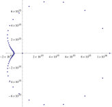
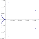
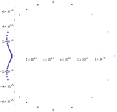
Figure 3: The distribution of the eigenvalues of the operator $A(N,s,m)$ in (3.12) for large value of $s$ and $m$, but fixed, and increasing values of $N=60,120,240$ from Table 3. The spectrum represents a leaf of a large radius proportional to $\lambda_{max}\approx m$ and a very small eigenvalue at the origin $\lambda_{min}\approx m^{-N+1}$. With increasing $N$ the “stem of the leaf” becomes more pronounced on the left hand side of the spectral curve.

Thus the case of $m=1$ simply corresponds to the original matrix (2.6). It is most advantageous to take large values of $m$, but preferably keeping $Nm<p$, such as to have an unambiguous correspondence between the continuous system (1.1) and the discrete system on the rational sublattice. The distribution of the eigenvalues of the operator $A(N,s,m)$ for the values of s and m which are given in Table 3 are presented on Fig.3. The spectrum for the increasing values of $N=60,120,240$ is shown in sequence, from left to right. The spectrum represent a leaf of a large radius proportional to $\lambda_{max}\approx m$ and very small eigenvalue at the origin $\lambda_{min}\approx m^{-N+1}$. With increasing $N$ the “stem of the leaf” becomes more pronounced on the left hand side of the spectral curve.

Size	Magic	Magic	Entropy	Log of the period q
N	$m$	s		$\approx\log_{10}(q)$
8	$m=2^{53}+1$	s=0	220.4	129
17	$m=2^{36}+1$	s=0	374.3	294
40	$m=2^{42}+1$	s=0	1106.3	716
60	$m=2^{52}+1$	s=0	2090.5	1083
96	$m=2^{55}+1$	s=0	3583.6	1745
120	$m=2^{51}+1$	s=1	4171.4	2185
240	$m=2^{51}+1$	s=487013230256099140	8679.2	4389

Table 3: Table of three-parameter MIXMAX generators $A(N,s,m)$ in (3.12). These generators have an advantage of having a very high quality sequence for moderate and small $N$. In particular, the smallest generator we tested, $N=8$, passes all tests in the BigCrush suite [23]. The period $q$ is defined in (2.10), (4.15).

A further possible generalization of the three-parameter family of operators is the following: the four-parameter operators $A(N,s,m,b)$ is constructed by replacing the sequence in the bands, below the diagonal, which is originally $3,4,5,...,N$ with the sequence $3m+b,4m+b,5m+b,...,Nm+b$, where $m$ and $b$ are some integers:

$$A(N,s,m,b)=\begin{pmatrix}1&1&1&1&...&1&1\\ 1&2&1&1&...&1&1\\ 1&3m+s+b&2&1&...&1&1\\ 1&4m+b&3m+b&2&...&1&1\\ 1&5m+b&4m+b&3m+b&...&1&1\\ &&&...&&&\\ 1&Nm+b&(N-1)m+b&(N-2)m+b&...&3m+b&2\end{pmatrix}.$$ (3.13)

This four-parameter family $A(N,s,m,b)$ reduces back to the three-parameter family $A(N,s,m)$ for $b=2-2m$. It is the case that some of these four-parameter generators, for specially chosen $m$ and $b$, allow efficient computer multiplication - the property which plays an essential role if one tries to use these operators for Monte-Carlo simulations.

4 Computer Implementation. MIXMAX Random Number Generator

In a typical computer implementation [3, 38] of the periodic trajectories of the automorphism (1.1) the initial vector

$$u^{(k)}=(u^{(k)}_{1},...,u^{(k)}_{N})$$

has a rational components $u^{(k)}_{i}=a^{(k)}_{i}/p$, where $a^{(k)}_{i}$ and $p$ are natural numbers and $i=1,...,N$. Therefore it is convenient to represent $u^{(k)}_{i}$ by its numerator $a^{(k)}_{i}$ in computer memory and define the iteration in terms of $a^{(k)}=(a^{(k)}_{1},...,a^{(k)}_{N})$ [3, 16]:

$$a^{(k+1)}_{i}=\sum_{j=1}^{N}A_{ij}\,a^{(k)}_{j}~{}~{}~{}\textrm{mod}~{}p~{},~{}~{}~{}~{}~{}~{}~{}k=0,1,2,....$$ (4.14)

If the denominator $p$ is taken to be a prime number [3, 16, 38], then the recursion is realised on extended Galois field $GF[p^{N}]$ [20, 21] and it allows to find the period of the trajectory $q$ in terms of $p$ and the properties of the characteristic polynomial $P(x)$ of the matrix $A$ [3, 16, 26, 38]. If the characteristic polynomial $P(x)$ of some matrix $A$ is primitive in the extended Galois field $GF[p^{N}]$, then [16, 19, 20, 26, 27]:

$$A^{q}=p_{0}~{}\mathbb{I}~{}~{}\textrm{ where}~{}~{}q=\frac{p^{N}-1}{p-1}~{},$$ (4.15)

where $p_{0}$ is a free term of the polynomial $P(x)$ and is a primitive element of $GF[p]$. Since our matrix $A$ has $p_{0}=\mathop{\rm Det}A=1$, the polynomial $P(x)$ of $A$ cannot be primitive. The solution suggested in [3] is to define the necessary and sufficient conditions for the period $q$ to attain its maximum, and they are [3]:

1. $A^{q}=\mathbb{I}~{}(mod~{}p)$,   where $q=\frac{p^{N}-1}{p-1}$.

2. $A^{q/r}\neq\mathbb{I}~{}(mod~{}p)$,     for any $r$ which is a prime divisor of $q$ .

The first condition is equivalent to the requirement that the characteristic polynomial is irreducible. The second condition can be checked if the integer factorisation of $q$ is available [3], then the period of the sequence is equal to (4.15) and is independent of the seed. There are precisely $p-1$ distinct trajectories which together fill up all states of the $GF[p^{N}]$ lattice:

$$q~{}(p-1)=p^{N}-1.$$ (4.16)

In [3] the actual value of $p$ was taken as $p=2^{61}-1$, the largest Mersenne number that fits into an unsigned integer on current 64-bit computer architectures. For the purposes of generating pseudo-random numbers with this method, one chooses any initial vector $a^{(0)}$, called the ”seed”, with at least one non-zero component.

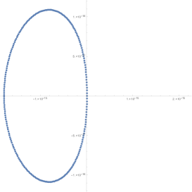
Figure 4: The distribution of the eigenvalues of the inverse operator $A^{-1}(N,s,m)$ of (3.12) for large values $N=240,s=487013230256099140$ and $m=2^{51}+1$.

The commonly-used RNGs based on a linear recurrence typically reach the maximal period of $p^{N}-1$ using the primitive elements of $GF[p^{N}]$. They use either a large prime number $p$ as in [23, 27, 28, 29, 30], or $p=2$ as in [32, 33, 34, 35].

The results of the last two sections allow to disclose some additional parameter values for the MIXMAX generator, in addition to those found in [3]. The properties of the MIXMAX generators improve appreciably with $N$, the size of the matrix, and therefore we undertook a search for large values of $N$ and some small values of the parameter $s$. Because the speed of the generator does not depend on $N$, these generators are useful if the dimension $D$ of the Monte-Carlo integration is large but finite, in which case one would like to choose $N\geq D$. If a generator with such large $N$ is available, then the convergence of the Monte-Carlo result to the correct value and with a residual which is normally distributed is assured. The latter guarantee is given by the theorem of Leonov [22, 4].

Our search of the parameters for the MIXMAX generator $A(N,s)$ with large $N$ and maximal period has yielded the values presented in the Table 2. As one can deduce from this data, the entropy is linearly increasing with $N$ (2.9). As it was demonstrated in [3], the Kolmogorov entropy, which needs to be greater than about $h(A)\approx 50$ for the generator to be empirically acceptable. Therefore it should not be surprising that for all of these generators, the sequence passes all tests in the BigCrush suite [23]. For the largest of them $N=44851$, the period is a number of nearly a million digits. If an increase in entropy is desired without increasing the size of the matrix $N$, it is now possible to search for large $s$ as well. The combinations of $N$ and $s$ which we found to be useful in this regard are presented in Table 1. The generator with $N=256$ and $s=487013230256099064$ has the best combination of speed, reasonable size of the state, and availability for implementing the parallelization by skipping and is currently available generator in the ROOT and CLHEP software packages at CERN for scientific calculation [39, 40, 41].

For the three-parameter family $A(N,s,m)$ of the MIXMAX generators the convenient values of the parameters are provided in Table 3. The efficient implementation in software can be achieved for some particularly convenient values of $m$ of the form $m=2^{k}+1$ [38]. Inspecting the data in the Table 3 one can get convinced that the system with $N=240,s=487013230256099140$ and $m=2^{51}+1$ has the best stochastic properties within the $A(N,s,m)$ family of operators. It is also obvious that the record value of the entropy $h(A)=28704.6$ which we achieved for the generator $A(N,s)$ with $N=44851,~{}s=-3$ remains the biggest and required few months of computer search.

5 Acknowledgement

This work was supported in part by the European Union’s Horizon 2020 research and innovation programme under the Marie Skĺodowska-Curie Grant Agreement No 644121.

6 Note Added

In this note we shall provide some additional comments.

The phase space of the C-systems under consideration (1.1 ) is a $N$-dimensional torus [1, 2, 3, 4], appearing at factorisation of the Euclidean space $E^{N}$ with coordinates $u=(u_{1},...,u_{N})$ over an integer lattice ${\cal Z}^{N}$. The coordinates $u$ on a torus are rational and irrational numbers. The operator $A$ acts on the initial vector $u^{(0)}$ and produces a phase space trajectory $u^{(n)}=A^{n}u^{(0)}$ on a torus. The trajectories of a C-system can be periodic and non-periodic. All trajectories which start from vectors $u^{(0)}$ which have rational coordinates, and only they, are periodic [1, 4]. The rational numbers are everywhere dense on the phase space of a torus and the periodic trajectories of the C-systems follow the same pattern and are everywhere dense [1], like rational numbers on a real line.

It is important now to raise the following fundamental question: can one approximate, and approximate uniformly, non-periodic trajectories of a C-system by using periodic trajectories of the same C-system? The answer is yes [1].

The trajectories which start from the irrational coordinates are uniformly distributed over the phase space on a torus and the main goal is to approximate, and approximate uniformly, these non-periodic trajectories. Therefore what we suggested in our preprint articles which were released in 1986 [2] and finally published in 1991 is to use the periodic trajectories of a C-system to approximate, as well as possible, the non-periodic, uniformly distributed trajectories of the same C-system. The periodic and non-periodic trajectories of a C-system should not be separated from each other within the C-system, they are in a harmonic union, as the rational and irrational numbers on a real line are.

We shall provide an example from calculus which may help to understand this harmonic union of trajectories. A good illustration example will be the approximation of the non-algebraic, transcendental number $\pi$ by rational numbers, which was the aim of Archimedes, $3{1\over 7}<\pi<3{10\over 71}$, of Ramanujan and the series of Leibniz:

$$\pi=4\sum^{\infty}_{n=0}{(-1)^{n}\over 2n+1}=4(1-{1\over 3}+{1\over 5}-.....)~{}.$$

One should ask: is this representation of $\pi$ in terms of rational numbers useful to us, humans, who are unable to embrace the number $\pi$ on a computer? It seems that it is a unique and useful way to grasp the number $\pi$, and, indeed, 13.3 trillion digits of $\pi$ were computed in October 2014. The same is true for the C-systems, the aim is to ”follow” the non-periodic trajectories for as long and as closely as possible by the periodic trajectories. The analogy will be complete if one recalls that the $\pi=3.14~{}....$ expressed in terms of decimal digits, is a non-periodic number, while the rational numbers are periodic. In this case we have approximation of a non-periodic number by a periodic.

It is therefore important to learn how dense are the periodic trajectories populating the phase space of a C-system and how this density is correlated with the entropy. The formula (1.5) describes the asymptotic distribution of the periodic trajectories of the length $q$, quantifying the rate at which they occur (see [4] and references therein). The asymptotic formula (1.5) approximates $\pi(q)$ in the sense that the relative error of this approximation approaches zero as $q$ tends to infinity, but does not say anything about the limit of the difference

$$\pi(q)-{e^{q\ h(A)}\over q}.$$

A good analogy will be the prime number theorem. There are infinitely many primes, as demonstrated by Euclid around 300 BC and the prime number theorem describes the asymptotic distribution of the prime numbers among the positive integers.

In this article we calculated some of the periods and it is obviously a nontrivial task. The Table 2 which presents the specific values of $N$ and $s$ and requires development of a computer code and months of computer time, the task which is analogous of searching large prime numbers. For the MIXMAX generator one should find those values of $N$ and $s$ for which all the necessary conditions are fulfilled. The fact that here we reached a period which is a million digits was not a ”sport” achievement but the ability to ”follow” a non-periodic trajectory as long as possible. The ability to increase further the dimension $N$, the entropy and the periods is a priceless advantage of the MIXMAX family of RNGs allowing them, in principle, and it is justified theoretically, to pass even stronger tests [36, 37].

References

- [1] D. V. Anosov, Geodesic flows on closed Riemannian manifolds with negative curvature, Trudy Mat. Inst. Steklov., Vol. 90 (1967) 3 - 210
- [2] G. Savvidy and N. Ter-Arutyunyan-Savvidy, On the Monte Carlo simulation of physical systems, J.Comput.Phys. 97 (1991) 566; Preprint EFI-865-16-86-YEREVAN, Jan. 1986. 13pp.
- [3] K.Savvidy, The MIXMAX random number generator, Comput.Phys.Commun. 196 (2015) 161-165. (http://dx.doi.org/10.1016/j.cpc.2015.06.003); arXiv:1404.5355
- [4] G. Savvidy, Anosov C-systems and random number generators, to be published in Theor.Math.Phys. arXiv:1507.06348 [hep-th].
- [5] G.Savvidy, The Yang-Mills mechanics as a Kolmogorov K-system, Phys.Lett.B 130 (1983) 303
- [6] G. Savvidy, Classical and Quantum Mechanics of Nonabelian Gauge Fields, Nucl. Phys. B 246 (1984) 302.
- [7] V.Gurzadyan and G.Savvidy, Collective relaxation of stellar systems, Astron. Astrophys. 160 (1986) 203
- [8] A.N. Kolmogorov, New metrical invariant of transitive dynamical systems and automorphisms of Lebesgue spaces, Dokl. Acad. Nauk SSSR, 119 (1958) 861-865
- [9] A.N. Kolmogorov, On the entropy per unit time as a metrical invariant of automorphism, Dokl. Acad. Nauk SSSR, 124 (1959) 754-755
- [10] Ya.G. Sinai, On the Notion of Entropy of a Dynamical System, Doklady of Russian Academy of Sciences, 124 (1959) 768-771.
- [11] V.A. Rokhlin, On the endomorphisms of compact commutative groups, Izv. Akad. Nauk, vol. 13 (1949), p.329
- [12] V.A. Rokhlin, On the entropy of automorphisms of compact commutative groups, Teor. Ver. i Pril., vol. 3, issue 3 (1961) p. 351
- [13] Ya. G. Sinai, Proceedings of the International Congress of Mathematicians, Uppsala (1963) 540-559.
- [14] A. L. Gines, Metrical properties of the endomorphisms on m-dimensional torus, Dokl. Acad. Nauk SSSR, 138 (1961) 991-993
- [15] N. Akopov, G. Savvidy and N. Ter-Arutyunyan-Savvidy, Matrix generator of pseudorandom numbers, J.Comput.Phys. 97, 573 (1991)
- [16] G. G. Athanasiu, E. G. Floratos, G. K. Savvidy K-system generator of pseudorandom numbers on Galois field, Int. J. Mod. Phys. C 8 (1997) 555-565; arXiv:physics/9703024
- [17] R.Bowen, Equilibrium States and the Ergodic Theory of Anosov Diffeomorphisms. (Lecture Notes in Mathematics, no. 470: A. Dold and B. Eckmann, editors). Springer-Verlag (Heidelberg, 1975), 108 pp.
- [18] R.Bowen, Periodic orbits for hyperbolic flows, Amer. J. Math.,94 (1972) 1-30.
- [19] R. Lidl and H. Niederreiter, Finite Fields, Addison-Wesley, Reading, MA, 1983, see also Finite fields, pseudorandom numbers, and quasirandom points, in : Finite fields, Coding theory, and Advance in Communications and Computing. (G.L.Mullen and P.J.S.Shine, eds) pp. 375-394, Marcel Dekker, N.Y. 1993.
- [20] H.Niederreiter, A pseudorandom vector generator based on finite field arithmetic, Mathematica Japonica, 31 (1986) 759-774.
- [21] N. Niki, Finite field arithmetic and multidimensional uniform pseudorandom numbers (in Japanese), Proc. Inst. Statist. Math. 32 (1984) 231.
- [22] V. P. Leonov, On the central limit theorem for ergodic endomorphisms of the compact commutative groups, Dokl. Acad. Nauk SSSR, 124 No: 5 (1969) 980-983
- [23] P. L’Ecuyer and R. Simard, TestU01: A C Library for Empirical Testing of Random Number Generators, ACM Transactions on Mathematical Software, 33 (2007) 1-40.
- [24] P. L’Ecuyer. Random number generation. In J. E. Gentle, W. Haerdle, and Y. Mori, editors, Handbook of Computational Statistics, pages 35?71. Springer-Verlag, Berlin, second edition, 2012.
- [25] P. L’Ecuyer, D. Munger, B. Oreshkin, and R. Simard. Random numbers for parallel computers: Requirements and methods, with emphasis on GPUs, 2015. revision submitted, http://www.iro.umontreal.ca/ lecuyer/myftp/papers/parallel-rng-imacs.pdf.
- [26] J. D. Alanen and D. E. Knuth. Tables of finite fields, SANKHYA: The Indian Journal of Statistics, Series A, 26 (1964) 305-328.
- [27] P. L’ Ecuyer. Good parameters and implementations for combined multiple recursive random number generators. Operations Research 47 (1) (1999) 159-164.
- [28] H. Grothe. Matrix generators for pseudo-random vectors generation, Statistische Hefte 28 (1987) 233-238.
- [29] D. E. Knuth. The Art of Computer Programming, Volume 2: Semi-numerical Algorithms. Addison-Wesley, Reading, MA, third edition, 1998.
- [30] P. L’Ecuyer. Random numbers for simulation. Communications of the ACM, 33(10) (1990) 85-97.
- [31] P. L’Ecuyer. Combined multiple recursive random number generators. Operations Research, 44(5) (1996) 816-822.
- [32] P. L’Ecuyer. Tables of maximally equidistributed combined LFSR generators. Mathematics of Computation, 68(225) (1999) 261-269.
- [33] M. Matsumoto and T. Nishimura. Mersenne twister: A 623-dimensionally equidistributed uniform pseudo-random number generator. ACM Transactions on Modelling and Computer Simulation, 8(1) (1998) 3-30.
- [34] T. Nishimura. Tables of 64-bit Mersenne twisters. ACM Transactions on Modeling and Computer Simulation, 10(4) (2000) 348-357.
- [35] F. Panneton, P. L’Ecuyer, and M. Matsumoto. Improved long-period generators based on linear recurrences modulo 2. ACM Transactions on Mathematical Software, 32(1) (2006) 1-16.
- [36] N. Marwan, M. C. Romano, M. Thiel, and J. Kurths. Recurrence plots for the analysis of complex systems. Physics Reports, 438 (2007) 237-329.
- [37] L. De Micco, H. A. Larrondo, A. Plastino, and O. A. Rosso. Quantiers for randomness of chaotic pseudo random number generators. Philosophical Transactions of the Royal Society A 367 (2009) 3281-3296.
-
[38]
HEPFORGE.ORG, http://mixmax.hepforge.org;
http://www.inp.demokritos.gr/~savvidy/mixmax.php - [39] MIXMAX workshop: https://indico.cern.ch/event/404547
-
[40]
ROOT, Release 6.04/06 on 2015-10-13,
https://root.cern.ch/doc/master/mixmax_8h_source.html -
[41]
GEANT/CLHEP, Release 2.3.1.1, on November 10th, 2015
http://proj-clhep.web.cern.ch/proj-clhep/