Analysis of structural correlations in a model binary 3D liquid through the eigenvalues and eigenvectors of the atomic stress tensors

Abstract

It is possible to associate with every atom or molecule in a liquid its own atomic stress tensor. These atomic stress tensors can be used to describe liquids’ structures and to investigate the connection between structural and dynamic properties. In particular, atomic stresses allow to address atomic scale correlations relevant to the Green-Kubo expression for viscosity. Previously correlations between the atomic stresses of different atoms were studied using the Cartesian representation of the stress tensors or the representation based on spherical harmonics.

In this paper we address structural correlations in a model 3D binary liquid using the eigenvalues and eigenvectors of the atomic stress tensors. Thus correlations relevant to the Green-Kubo expression for viscosity are interpreted in a simple geometric way. On decrease of temperature the changes in the relevant stress correlation function between different atoms are significantly more pronounced than the changes in the pair density function. We demonstrate that this behaviour originates from the orientational correlations between the eigenvectors of the atomic stress tensors.

We also found correlations between the eigenvalues of the same atomic stress tensor. For the studied system, with purely repulsive interactions between the particles, the eigenvalues of every atomic stress tensor are positive and they can be ordered: $\lambda_{1}\geq\lambda_{2}\geq\lambda_{3}\geq 0$. We found that, for the particles of a given type, the probability distributions of the ratios $(\lambda_{2}/\lambda_{1})$  and $(\lambda_{3}/\lambda_{2})$  are essentially identical to each other in the liquids state. We also found that $\lambda_{2}$ tends to be equal to the geometric average of $\lambda_{1}$ and $\lambda_{3}$. In our view, correlations between the eigenvalues may represent “the Poisson ratio effect” at the atomic scale.

I Introduction

Despite many years of investigations there is still no commonly accepted vision of the slowdown mechanism in supercooled liquids Ediger20121; Biroli20131. It is natural to expect that in order to understand the behaviour of supercooled liquids and the phenomenon of the glass transition it is necessary to be able to describe structural changes in a way that would allow to make connection to the dynamical properties EMa20111; ChenYQ2013; Tanaka20131; Wei20151.

Viscosity represents a standard parameter that is used to characterize dynamical slowdown in supercooled liquids. In molecular dynamics simulations liquids’ viscosities are commonly calculated using the Green-Kubo expression Green1954; Kubo1957; Helfand1960; HansenJP20061; Boon19911; EvansDJ19901:

$$\eta=\frac{V}{k_{\scalebox{0.5}{B}}T}\int_{0}^{\infty}<\Pi^{xy}(t_{o})\Pi^{xy}(t_{o}+t)>_{t_{o}}dt\;\;,$$ (1)

where $k_{\scalebox{0.5}{B}}$-is the Boltzmann constant, $T$ -is the temperature, $V$-is the volume of the system, $\Pi^{xy}(t)$-is the value of the $xy$ component of the macroscopic stress tensor at time $t$. Expression (1) is the limit for zero-frequency and zero-wavevector viscosity $\eta(\omega=0,q=0)$ HansenJP20061; Boon19911; EvansDJ19901.

For a given interaction potential, the macroscopic stress tensor $\Pi^{xy}(t)$ depends on particles’ velocities and coordinates. In the past there have been multiple investigations of the behaviour of the integration kernel in (1) Hoheisel19881. In particular, it has been found that in supercooled liquids the value of the correlation function $<\Pi^{xy}(t_{o})\Pi^{xy}(t_{o}+t)>_{t_{o}}$ is almost completely determined by the liquids structure, i.e., by particles coordinates, while the contribution from the terms associated with the particles’ velocities usually represents less than $5\%$ of the correlation function value Hoheisel19881. For this reason we neglect the velocity dependent terms and provide a simple version of the definition of the macroscopic stress tensor. Thus, as it was discussed before, the macroscopic stress tensor can be written as the sum of the atomic level stress elements Levashov20111; Levashov2013:

$$\Pi^{xy}(t)=\frac{1}{V}\sum_{i=1}^{N}s_{i}^{xy},$$ (2)

$$s_{i}^{xy}=\sum_{j\neq i}\left(\frac{dU_{ab}(r_{ij})}{dr_{ij}}\right)\left(\frac{r_{ij}^{a}r_{ij}^{b}}{r_{ij}}\right),$$ (3)

where $U_{ab}(r_{ij})$ is the interaction pair potential between the particles of type $a$ and $b$, while $\bm{r_{ij}}=\bm{r_{j}-r_{i}}$ is the radius vector from particle $i$ to particle $j$. The sum over $j$ in (3) is over all particles with which particle $i$ interacts.

In principle, expressions (1,2,3) establish the relationship between the structure and the dynamic quantity, i.e., viscosity. However, the form of the expressions (1,2,3) does not provide an explicit answer with respect to what kind of structural correlations determine viscosity. There were studies that addressed how local structural perturbations affect the the stress fields in glasses and liquids Picard20041; Tanguy20061; Maloney20061; Lemaitre20071; Tsamados20081; Lemaitre20091; Chattorai20131; Puosi20141; Lemaitre20141. Yet, the geometric meaning of the atomic scale correlations relevant to the Green-Kubo expression for viscosity has not been completely elucidated. What is meant by the last statement will become more clear from the following.

In several previous publications behaviour of the correlation function $<\Pi^{xy}(t_{o})\Pi^{xy}(t_{o}+t)>_{t_{o}}$ has been studied from an atomic scale perspective Levashov20111; Levashov2013; Levashov20141; Levashov2014B; Bin20151. In these studies macroscopic shear stress correlation function in (1) has been expanded into the correlation functions, $\langle s_{i}^{xy}s_{j}^{xy}\rangle$ between the atomic level stress elements from (2,3). In this way, in particular, a relationship between the propagation of shear stress waves and viscosity has been demonstrated on atomic scale Levashov20111; Levashov2013; Levashov20141; Levashov2014B.

In order to understand the correlation function $\langle s_{i}^{xy}s_{j}^{xy}\rangle$, as follows from this paper, it is useful to realize that the form $\langle s_{i}^{xy}s_{j}^{xy}\rangle$ reflects not only the nature of the physical correlations in liquids, but also the properties of the chosen Cartesian representation. On the other hand, it is a common practice in considerations of tensors to speak about their properties in terms of representation-invariant parameters Ruiz2005; Algebra. Surprisingly (to the best of our knowledge) the correlation function $\langle s_{i}^{xy}s_{j}^{xy}\rangle$ has not been studied before in 3D in terms of representation-invariant variables. Our present paper is devoted to these kind of investigations.

Our approach is based on the concept of atomic stress elements (or atomic level stresses) Egami19801; Egami19802; Egami19821. In the framework of this approach the atomic environment of every atom is described by a symmetric and real atomic stress tensor. In this paper we define the atomic stress tensor in a way which is somewhat different from the previously used definition Egami19801; Egami19802; Egami19821; Chen19881; Levashov2008B. We explain this difference in the following. Thus, for an atom $i$ we define its atomic stress tensor as:

$$\sigma_{i}^{\alpha\beta}=-\frac{1}{2\langle V_{i}\rangle}\sum_{j\neq i}\left[\frac{dU_{ab}(r_{ij})}{dr_{ij}}\right]\left(\frac{r_{ij}^{\alpha}r_{ij}^{\beta}}{r_{ij}}\right)\;,\;\;$$ (4)

where $\langle V_{i}\rangle$ is the average atomic volume, $\langle V_{i}\rangle\equiv 1/\rho_{o}$, while $\rho_{o}$ is the average atomic number density. Note that the definition without $\langle V_{i}\rangle$ and with the opposite sign corresponds to the atomic stress element from (2,3) Levashov2013; Levashov20111. Also note that $\alpha$-component of the force acting on particle $i$ from particle $j$ is $f^{\alpha}_{ij}=\left[dU_{ab}(r_{ij})/dr_{ij}\right]\left(r_{ij}^{\alpha}/r_{ij}\right)$. Finally note that the atomic stress tensor (4) is symmetric with respect to the indexes $\alpha$ and $\beta$. Thus in 3D it has 6 independent components Egami19801; Egami19802; Egami19821; Chen19881; Levashov2008B.

We introduced the $\langle V_{i}\rangle$ in (4) in order to use variables, $\sigma_{i}^{\alpha\beta}$, that have units of stress. Since, for a given density, $\langle V_{i}\rangle$ is just a constant its introduction does not affect any conclusions. In comparison to the previous definition Egami19801; Egami19802; Egami19821; Chen19881; Levashov2008B we also introduced the minus sign in (4). Our definition makes an atom under compression to have a positive pressure, while under the previous definition atoms under compression had negative pressure. Thus, the minus sign in (4) is also only a matter of convenience, which makes the results look more intuitive.

In the previous definition of the atomic level stresses instead of a constant $\langle V_{i}\rangle$ was used essentially the volume of the Voronoi cell of an atom Egami19801; Egami19802; Egami19821; Chen19881; Levashov2008B. Thus every atom, in the previously used definition, had its own characteristic volume. We, in our considerations, avoid using the atom-dependent Voronoi volume because it is not present in the expressions for viscosity (1,2,3). Thus we would like to use variables which are directly related to viscosity, but at the same time we want them to have convenient “stress” units. For this reason we introduced the constant multiplication factor $\langle V_{i}\rangle$.

The concept of atomic level stresses was introduced to describe structures of metallic glasses and their liquids Egami19801; Egami19802; Egami19821. There are several important results associated with this concept. One result is the equipartition of the atomic level stress energies in liquids Egami19821; Chen19881; Levashov2008B. Thus, the energies of the atomic level stress components can be defined and it was demonstrated, for the studied model liquids in 3D, that the energy of every stress component is equal to $k_{\scalebox{0.5}{B}}T/4$. Thus the total stress energy, which is the sum of the energies of all six stress components, is equal to $6\cdot k_{\scalebox{0.5}{B}}T/4=(3/2)k_{\scalebox{0.5}{B}}T$, i.e., the potential energy of a classical 3D harmonic oscillator. An explanation of this result has been suggested Egami19821; Chen19881; Levashov2008B. Then there was an attempt to describe the glass transition and fragilities of liquids using atomic level stresses Egami20071. Another result is related to the Green-Kubo expression for viscosity. Thus the macroscopic stress correlation function that enters into the Green-Kubo expression for viscosity was decomposed into the correlation functions between the atomic stress elements. Considerations of the obtained atomic stress correlation functions demonstrated the relationship between the propagation and dissipation of shear waves and viscosity. This result, after all, is not surprising in view of the existing generalized hydrodynamics and mode-coupling theories HansenJP20061; Boon19911. However, in Ref.Levashov2013; Levashov20111; Levashov20141; Levashov2014B the issue has been addressed from a new perspective and the relationship between viscosity and shear waves was demonstrated very explicitly at the atomic level.

Since the atomic stress tensor is real and symmetric it can be diagonalized and its eigenvalues and eigenvectors can be found Algebra. In the Cartesian coordinate frame based on the eigenvectors the atomic stress tensor is diagonal with the eigenvalues on the diagonal. Thus six stress elements of the symmetric atomic stress tensor (in our reference coordinate frame) contain the information about the eigenvalues and orientations of the eigenvectors. It follows from this viewpoint that in the approach based on considerations of the atomic stresses it is possible in 3D to associate with every atom (and its environment) an ellipsoid whose axes have the lengths of the eigenvalues and whose orientation is described by its eigenvectors.

Analysis in terms of the eigenvalues and eigenvectors of the atomic stresses represents simple, geometric and representation-invariant approach that can be used to describe liquids’ structures. In this paper we express, in particular, the correlation function $\langle\sigma_{i}^{xy}\sigma_{j}^{xy}\rangle$ in terms of the correlation functions between the eigenvalues and the angles between the eigenvectors of atoms $i$ and $j$. This result provides a new insight into the nature of the structural correlations that determine the Green-Kubo correlation function. Our results show that on supercooling correlations in the orientations of the stress ellipsoids develop. These orientational correlations cause more significant changes in the $\langle\sigma_{i}^{xy}\sigma_{j}^{xy}\rangle$ correlation function than the changes associated with correlations between the eigenvalues.

Effectively this paper has four parts. In the first part we describe the formalism that allows to address structure of liquids in terms of the eigenvalues and eigenvectors of the atomic stresses. In the second part, using MD and MC simulations we analyse correlations between the eigenvalues of the same atomic stress tensor and some other related issues. In the third part, we present the results on correlations between the eigenvalues and eigenvectors of different atoms. The forth part contains appendices that provide additional analytical insights into the data obtained with computer simulations.

II Stress tensor ellipsoids

The atomic stress tensor, $\Sigma_{i}$, defined with equation (4) is real and symmetric. Thus it can be diagonalised and, in 3D, three real eigenvalues $\lambda^{1}_{i}$, $\lambda^{2}_{i}$, $\lambda^{3}_{i}$ and three real orthogonal eigenvectors of the stress tensor can be found Algebra. For this reason we can associate with every atom an ellipsoid with the axes of length $\lambda^{1}_{i}$, $\lambda^{2}_{i}$, $\lambda^{3}_{i}$. These axes are parallel to the corresponding eigenvectors. In the frame of the ellipsoid’s axes the stress tensor is diagonal.

In the following we refer to the coordinate frame based on the eigenvectors of atom $i$ as to the eigenframe of atom $i$. In a different reference coordinate frame for the normalized eigenvector $\bm{\bm{\hat{v}}}_{i}^{1}$ we introduce the following notations:

$$\bm{\bm{\hat{v}}}_{i}^{1}=\left(c_{i}^{11},c_{i}^{12},c_{i}^{13}\right)\;\;,\;$$ (5)

where the vector’s components are the directional cosines defined through the scalar products:

$$c_{i}^{11}=\bm{\bm{\hat{v}}}_{i}^{1}\bm{\hat{x}}\;,\;\;\;c_{i}^{12}=\bm{\bm{\hat{v}}}_{i}^{1}\bm{\hat{y}}\;,\;\;\;c_{i}^{13}=\bm{\bm{\hat{v}}}_{i}^{1}\bm{\hat{z}}\;\;.\;\;\;\;\;\;$$ (6)

Similar notations are assumed for the other two eigenvectors. Further we define the matrix of the column-eigenvectors, $V_{i}$, and the matrix of the eigenvalues, $\Lambda_{i}$:

$$V_{i}\equiv\begin{pmatrix}c_{i}^{11}&c_{i}^{21}&c_{i}^{31}\\ c_{i}^{12}&c_{i}^{22}&c_{i}^{32}\\ c_{i}^{13}&c_{i}^{23}&c_{i}^{33}\end{pmatrix}\;\;,\;\;\;\;\Lambda_{i}\equiv\begin{pmatrix}\lambda_{i}^{1}&0&0\\ 0&\lambda_{i}^{2}&0\\ 0&0&\lambda_{i}^{3}\end{pmatrix}\;\;.\;\;\;\;$$ (7)

If follows from the definitions of $V_{i}$, $\Lambda_{i}$, and the known relations from linear algebra that:

$$\sigma_{i}V_{i}=V_{i}\Lambda_{i}\;\;.\;\;$$ (8)

From (8) we get:

$$\Lambda_{i}=V_{i}^{T}\Sigma_{i}V_{i}\;\;,\;\;\;\;\;\;\;\Sigma_{i}=V_{i}\Lambda_{i}V_{i}^{T}\;\;,\;\;$$ (9)

where matrix $V_{i}^{T}$ is the transposed and also the inverse of $V_{i}$.

In our further considerations we use some well known results Ruiz2005; Algebra from linear algebra and tensor analysis about which we remind here. Let us suppose that the stress tensors of atoms $i$ in a particular coordinate frame is:

$$\Sigma_{i}\equiv\begin{pmatrix}\sigma_{i}^{x}&\tau_{i}^{xy}&\tau_{i}^{xz}\\ \tau_{i}^{xy}&\sigma_{i}^{y}&\tau_{i}^{yz}\\ \tau_{i}^{xz}&\tau_{i}^{yz}&\sigma_{i}^{z}\end{pmatrix}.\;\;\;\;$$ (10)

The equation (the determinant) for the eigenvalues of a $3\times 3$ real symmetric (stress) matrix can be written in terms of the rotational invariants, $I_{1}$, $I_{2}$, and $I_{3}$ as follows:

$$\lambda^{3}-I_{1}\lambda^{2}+I_{2}\lambda-I_{3}=0\;\;,\;\;$$ (11)

where (for briefness we omit index $i$):

$$I_{1}= +\sigma^{x}+\sigma^{y}+\sigma^{z}\;,\;\;$$ (12)

$$I_{2}= +\sigma^{x}\sigma^{y}+\sigma^{x}\sigma^{z}+\sigma^{y}\sigma^{z}$$

$$-(\tau^{xy})^{2}-(\tau^{xz})^{2}-(\tau^{yz})^{2}$$

$$I_{3}= +\sigma^{x}\sigma^{y}\sigma^{z}+2\tau^{xy}\tau^{xz}\tau^{yz}$$

$$-(\tau^{xy})^{2}\sigma^{z}-(\tau^{xz})^{2}\sigma^{y}-(\tau^{yz})^{2}\sigma^{x}\;\;.\;\;$$

If the eigenvalues are known then these invariants can be rewritten in terms of the eigenvalues:

$$I_{1}\;=\;\; \lambda_{1}+\lambda_{2}+\lambda_{3}\;,\;\;$$ (15)

$$I_{2}\;=\;\; \lambda_{1}\lambda_{2}+\lambda_{1}\lambda_{3}+\lambda_{2}\lambda_{3}\;,\;\;$$ (16)

$$I_{3}\;=\;\; \lambda_{1}\lambda_{2}\lambda_{3}\;.\;\;$$ (17)

For further convenience let us also notice that:

$$(I_{1})^{2}-3I_{2} =\lambda_{1}^{2}+\lambda_{2}^{2}+\lambda_{3}^{2}-\lambda_{1}\lambda_{2}-\lambda_{1}\lambda_{3}-\lambda_{2}\lambda_{3}$$

$$=\frac{1}{2}\left[(\lambda_{1}-\lambda_{2})^{2}+(\lambda_{1}-\lambda_{3})^{2}+(\lambda_{2}-\lambda_{3})^{2}\right]\;.$$

It is demonstrated in the following subsection that $(I_{1})^{2}-3I_{2}$ in (II) is essentially the square of the von Mises shear stress.

II.1 Elements of the atomic stress tensors in the spherical representation

Previously it has been argued that it is useful to assume that the nearest neighbour atomic environment of every atom is approximately spherical Egami19821; Chen19881; Levashov2008B. This assumption, in particular, allows to introduce and rationalise the concept of the atomic stress energies as excitations from some average atomic environment. The relevant derivation is based on the representation of the atomic stresses in terms of the spherical harmonics Egami19821; Chen19881. In the following sections we present the data that justify consideration of this approach in our context.

The atomic stress elements defined through (4) do not reflect the vision that the nearest neighbour atomic environment of every atom is approximately spherical (however good or bad this approximation is). The consideration of the atomic stresses in terms of the spherical harmonics leads to the following linear combinations of the Cartesian stress components that reflect the vision that atomic environment of every atom is approximately spherical:

$$p_{i}\equiv s_{0,i}\equiv\tfrac{1}{3}\left[\sigma^{x}_{i}+\sigma^{y}_{i}+\sigma^{z}_{i}\right]\;,\;\;\;\;$$ (22)

$$s_{1,i}\equiv\tau^{xy}_{i}\;,\;\;s_{2,i}\equiv\tau^{xz}_{i}\;,\;\;s_{3,i}\equiv\tau^{yz}_{i}\;,\;$$

$$s_{4,i}\equiv\tfrac{1}{2}\left(\sigma^{x}_{i}-\sigma^{y}_{i}\right)\;,\;$$

$$s_{5,i}\equiv\tfrac{1}{\sqrt{3}}\left[\sigma_{i}^{z}-\tfrac{1}{2}\left(s^{x}_{i}+s^{y}_{i})\right)\right]\;,\;$$

Formulas (22,22,22,22) define one pressure component, $p_{i}\equiv s_{0,i}$, and 5 equivalent to each other shear stress components that reflect sphericity of the atomic environment of atom $i$ Egami19821; Chen19881; Levashov2008B: The notations that we use are slightly different from those used previously Egami19821; Chen19881; Levashov2008B. See Ref.sphstress1 for the details.

In the following we use the notation (abbreviation) $\sigma_{i}^{sph}$s  for the “spherical stress components”.

Vice versa from (22,22,22,22) we obtain:

$$\sigma^{x}_{i}=s_{0,i}-\tfrac{1}{\sqrt{3}}s_{5,i}+s_{4,i}\;,\;\;$$ (23)

$$\sigma^{y}_{i}=s_{0,i}-\tfrac{1}{\sqrt{3}}s_{5,i}-s_{4,i}\;,\;\;\;\;$$ (24)

$$\sigma^{z}_{i}=s_{0,i}+\tfrac{2}{\sqrt{3}}s_{5,i}\;,\;\;$$ (25)

$$\tau^{xy}_{i}=s_{1,i}\;,\;\;\;\tau^{xz}_{i}=s_{2,i}\;,\;\;\;\tau^{yz}_{i}=s_{3,i}\;.\;\;\;\;\;\;\;$$ (26)

It was argued in Ref.Egami19821 that the atomic stress tensor components $s_{0,i},\;s_{1,i},\;s_{2,i},\;s_{3,i},\;s_{4,i},\;s_{5,i}$ should be independent from each other in the linear approximation. This assumption plays an important role in rationalizing why the energies of these stress components are equal to each other and in explaining why the energy of every component in the liquid state is equal to $\tfrac{1}{4}k_{\scalebox{0.5}{B}}T$. The results from numerical simulations presented in Ref.Chen19881; Levashov2008B support this assumption. In this paper we address the issue of independence of the $\sigma_{i}^{sph}$s  from a new perspective, i.e., from the perspective of the probability distributions of the eigenvalues of the atomic stresses.

In the eigenframe of its eigenvectors an atomic stress tensor is characterised by its 3 eigenvalues $\lambda_{1}$, $\lambda_{2}$, and $\lambda_{3}$. Let us now consider this stress tensor in a different coordinate frame. It is straightforward to show that in any coordinate frame the sum of the squares of the shear stress components in the spherical representation is equal to:

$$\left(s_{vM,i}\right)^{2} \equiv\frac{1}{5}\sum_{n=1}^{n=5}\left(s_{n,i}\right)^{2}$$

$$=\frac{1}{30}\left[(\lambda_{1}-\lambda_{2})^{2}+(\lambda_{1}-\lambda_{3})^{2}+(\lambda_{2}-\lambda_{3})^{2}\right]\;.$$

Expression (II.1) is essentially the definition of the von Mises shear stress. It follows from (II.1) that the square of the von Mises shear stress is rotationally invariant. It follows from the comparison of (II.1) with (II) that the stress tensor invariant $I_{2}$ is related to the von Mises shear stress.

Let us evaluate the value of the square of a shear stress component averaged over all possible orientations of the reference coordinate frame. It follows from formulas (51,56), that we derive further, that this average value is equal to the square of the von Mises shear stress from (II.1):

$$\langle\left(s_{n,i}\right)^{2}\rangle_{\Omega}=\left(s_{vM,i}\right)^{2}\;.\;\;\;\;\;\;\;\;$$ (28)

In the previous considerations of the atomic stresses in glasses and liquids the atomic level pressure and von Mises shear stress have been studied Egami19821; Chen19881; Levashov2008B. In particular, studies of the equipartition of the atomic stress energies can be considered as the studies of the atomic von Mises shear stresses. In contrast, the role of the third invariant $I_{3}$ from (17) has not been addressed previously. It is clear from (17) that $I_{3}$ essentially represents the volume of the ellipsoid with axes $\lambda_{1}$, $\lambda_{2}$, $\lambda_{3}$. The value of $I_{3}$ can be used, for example, in order to characterize the relative scale of the shear deformation. For example, one can use the geometric average, i.e., $\lambda_{geom}\equiv\left(\lambda_{1}\lambda_{2}\lambda_{3}\right)^{1/3}$ in order to normalize the von Mises shear stress. Similarly the difference between the pressure (arithmetic average of the eigenvalues) and $\lambda_{geom}$ also gives certain measure of the deformation of the local atomic environment from the purely spherical state.

III Two Random Reference Models

As we already noted before, in the approach based on considerations of the atomic stresses the geometry of the nearest neighbour shell, if its orientation with respect to the reference coordinate frame is ignored, is characterised by only three numbers – three eigenvalues. Alternatively, it is possible to consider three invariants of the atomic stress tensor (12,II,II).

In considerations of the eigenvalues the first natural question to ask is: “What are their distributions?” The second question to ask is: “Are there correlations between the eigenvalues of the same atom?”

The issues related to the probability distributions ($PDs$) of the eigenvalues represent large field studied in mathematics and physics randommatrices; Wigner1967. One well known application is related to the studies of the PDs  of the energy levels which result from diagonalization of various Hamiltonians. In the context of supercooled liquids and the glass transition the Hessian matrix is routinely diagonalized in order to find the vibrational spectra of the studied systems amorhpous2001; Matsuoka2012.

One the other hand, we are familiar with only few papers in which the atomic stress tensors were diagonalized and the PDs  of their eigenvalues have been investigated Kust2003a; Kust2003b. It was demonstrated in those studies that there are correlations between the eigenvalues for several 2D and 3D mono-atomic and binary systems. However, the nature of those correlations is not understood, as the authors themselves point out Kust2003b.

Here we further investigate the correlations between the eigenvalues. In some of our considerations we use two modifications of the method suggested in Ref.Kust2003a; Kust2003b.

The idea of the first method is the following. From MD simulations it is possible to obtain the probability distribution ($PD$) for all eigenvalues without making the distinction which eigenvalue is the largest, the middle, or the smallest one. If the PD  for all eigenvalues is known, then it is possible to generate, using Monte Carlo technique, independent and random numbers whose PD  is the same as the PD  of the eigenvalues. Let us suppose that we generated three such numbers. Then, if needed, we can order them according to their magnitudes. In order to address correlations between the eigenvalues of the same atom, it is possible to compare the quantities of interest obtained directly from MD simulations with the same quantities obtained from the independent and random generation of the eigenvalues. This method, as far as we understand, is essentially equivalent to the method used in Ref.Kust2003a; Kust2003b. In the following we refer to this method as to the “$RI\lambda\;$approach” (Random and Independent for $\lambda$).

Another method that we employed combines the previous method with the idea that atomic stresses in the spherical representation (22,22,22,22) should be independent from each other in the linear approximation Egami19821; Chen19881; Levashov2008B. Thus, let us suppose that we obtained the PDs  of the atomic stress elements in the spherical representation from MD simulations. Using these PDs  we can generate independent and random spherical stresses in such a way that their PDs  correspond to those obtained in MD simulations. Using a particular random set of pressure and five spherical shear components we can form the random stress matrix in the Cartesian representation (23,24,25,26) which can be diagonalized. In this way we can obtain the eigenvalues from the independent and random selection of the $\sigma_{i}^{sph}$s. The PDs  of the eigenvalues obtained in this way can be compared with the PDs  of the eigenvalues obtained directly from MD simulations. It is also possible to compare the quantities of interest obtained from the independent and random selection of the $\sigma_{i}^{sph}$s  with the same quantities obtained directly from MD simulations. In the following we refer to this method as to the “$RI\sigma^{sph}\;$approach” (Random and Independent for the Spherical Stresses).

We conclude this section by describing the rejection method, i.e., the well known Monte Carlo algorithm that we used to generate random numbers with given PDs  numrecip. Let us suppose that some quantity $x$ has such probability distribution, $P(x)$, that we always have: $x_{min}\leq x\leq x_{max}$ and $0\leq P(x)\leq P_{max}$. Using a random number generator, which generates homogeneously distributed random numbers, we generate trial numbers $x_{trial}$ and $y_{trial}$ which lie in the intervals: $x_{min}\leq x_{trial}\leq x_{max}$ and $0\leq y_{trial}\leq P_{max}$. On the final step $x_{trial}$ is accepted into the randomly generated set of interest if $y_{trial}\leq P(x_{trial})$. Otherwise $x_{trial}$ is not accepted into the set.

IV Correlation functions

If the parameters of the stress tensor ellipsoids of atoms $i$ and $j$ are known then it is possible to study all kinds of correlations that take into account the eigenvalues and orientations of the eigenvectors of atoms $i$ and $j$. However, it is reasonable to study those atomic scale correlations which are related to the macroscopic physical quantities. For example, in order to study correlations related to viscosity it is necessary to express the correlation function $\left<\sigma_{i}^{xy}s_{j}^{xy}\right>$ in terms of the eigenvalues and angles that characterise orientations of the atomic stress ellipsoids.

If the atomic stress tensor, $\Sigma_{i}$, of atom $i$ is known in one (the 1st) coordinate frame then it also can be found in a different (the 2nd) coordinate frame. Thus:

$$\tilde{\Sigma}_{i}=R\Sigma_{i}R^{T}\;,\;$$ (29)

where the columns in the rotation matrix $R$ are the directional cosines of the 1st coordinate frame, $\bm{\hat{x}}$, $\bm{\hat{y}}$, $\bm{\hat{z}}$, with respect to the 2nd coordinate frame $\bm{\hat{\tilde{x}}}$, $\bm{\hat{\tilde{y}}}$, $\bm{\hat{\tilde{z}}}$. Note that expression (29) is essentially the same as the second expression in (9).

Let us suppose that we are interested in correlations between the parameters and orientations of the atomic stress ellipsoids of atoms $i$ and $j$ separated by radius vector $\bm{r}_{ij}$ . If the medium is isotropic then physically meaningful correlations can depend on distance $r_{ij}$, but should not depend on the direction of $\bm{r}_{ij}$ . For this reason it is reasonable to consider for every given pair of atoms $i$ and $j$ the directional coordinate “$\left\{\bm{r}_{ij}\right\}$ -frame” associated with the direction from atom $i$ to atom $j$.

IV.1 Directional coordinate frame associated with the direction from atom $i$ to atom $j$

Let us assume that $\bm{\hat{z}}\;$-axis of the directional coordinate “$\left\{\bm{r}_{ij}\right\}$ -frame” associated with the direction from atom $i$ to atom $j$ is along $\bm{r}_{ij}$ . Thus $\bm{\hat{x}}\;$and $\bm{\hat{y}}\;$-axes of the directional coordinate frame lie in the plane orthogonal to $\bm{r}_{ij}$ . Their precise directions will not be important to us as we are going to average over their orientations in the plane.

IV.2 Correlation function $\left<\tau_{i}^{xy}\tau_{j}^{xy}\right>\equiv\left<\sigma_{i}^{xy}\sigma_{j}^{xy}\right>$ in the directional coordinate frame

Let us express the product $\tau_{i}^{xy}\tau_{j}^{xy}\equiv\sigma_{i}^{xy}\sigma_{j}^{xy}$ in terms of the eigenvalues and the directional cosines of the eigenvectors in the directional $\left\{\bm{r}_{ij}\right\}$ -frame. The expressions derived below provide physical and representation-invariant insight into the correlations that determine viscosity.

Figure 1: Mutual orientation of the eigenvectors $V_{i}^{n}$ and $V_{j}^{m}$ is characterized by the angles $\psi_{i}^{n}$ and $\psi_{j}^{m}$ which they form with the direction $\bm{r}_{ij}$ and by the angle, $\delta_{ij}^{nm}$, between their projections on the plane orthogonal to $\bm{r}_{ij}$.

Further it is assumed that the directional cosines of the eigenvectors of atoms $i$ and $j$ in the $\left\{\bm{r}_{ij}\right\}$ -frame are known. Thus:

$$\bar{c}_{i}^{n1}=\sin(\psi_{i}^{n})\cos(\varphi_{i}^{n})\;,\;\;\;\;\;\bar{c}_{j}^{m1}=\sin(\psi_{j}^{m})\cos(\varphi_{i}^{n}+\delta_{ij}^{nm})\;,$$

$$\bar{c}_{i}^{n2}=\sin(\psi_{i}^{n})\sin(\varphi_{i}^{n})\;,\;\;\;\;\;\;\bar{c}_{j}^{m2}=\sin(\psi_{j}^{m})\sin(\varphi_{i}^{n}+\delta_{ij}^{nm})\;,$$

$$\bar{c}_{i}^{n3}=\cos(\psi_{i}^{n})\;,\;\;\;\;\;\;\;\;\;\;\;\;\;\;\;\;\;\;\bar{c}_{j}^{m3}=\cos(\psi_{j}^{m})\;.$$ (30)

In the expressions above $\psi_{i}^{n}$ and $\psi_{j}^{m}$ are the angles that $n$-th and $m$-th eigenvectors of atoms $i$ and $j$ form with the $\bm{\hat{z}}\;$-axis of the $\left\{\bm{r}_{ij}\right\}$ -frame. See Fig.1. According to the adopted convention, the angles $\psi_{i}^{n}$ and $\psi_{j}^{m}$ lie in the interval $\left(0,\tfrac{\pi}{2}\right)$. The angle $\varphi_{i}^{n}$ characterizes the orientation of the projection the $n$-th eigenvector of atom $i$ on the plane orthogonal to $\bm{r}_{ij}$ with respect to the $\bm{\hat{x}}\;$-axis of the $\left\{\bm{r}_{ij}\right\}$ -frame. It is also assumed in (30) that the projection of the $m$-th eigenvector of atom $j$ on the plane orthogonal to $\bm{r}_{ij}$ forms angle $\delta_{ij}^{nm}$ with the projection of the $n$-th eigenvector of atom $i$. The angle $\delta_{ij}^{nm}$ can be found from the scalar product of the eigenvectors’ projections on the plane orthogonal to $\bm{r}_{ij}$ . The bars over letters, like in $\bar{c}_{i}^{n1}$, signify that the bar-marked parameters are related to the $\left\{\bm{r}_{ij}\right\}$ -frame. Thus the matrices that rotate from the eigenframes of atoms $i$ and $j$ into the $\left\{\bm{r}_{ij}\right\}$ -frame are:

$$\bar{R}_{i}\equiv\begin{pmatrix}\bar{c}_{i}^{11}&\bar{c}_{i}^{21}&\bar{c}_{i}^{31}\\ \\ \bar{c}_{i}^{12}&\bar{c}_{i}^{22}&\bar{c}_{i}^{32}\\ \\ \bar{c}_{i}^{13}&\bar{c}_{i}^{23}&\bar{c}_{i}^{33}\\ \end{pmatrix}\;\;,\;\;\;\;\bar{R}_{j}\equiv\begin{pmatrix}\bar{c}_{j}^{11}&\bar{c}_{j}^{21}&\bar{c}_{j}^{31}\\ \\ \bar{c}_{j}^{12}&\bar{c}_{j}^{22}&\bar{c}_{j}^{32}\\ \\ \bar{c}_{j}^{13}&\bar{c}_{j}^{23}&\bar{c}_{j}^{33}\\ \end{pmatrix}\;\;.\;\;\;\;$$ (31)

It follows from (29,31) that:

$$\bar{\sigma}_{i}^{x}=\lambda_{i}^{1}\left(\bar{c}_{i}^{11}\right)^{2}+\lambda_{i}^{2}\left(\bar{c}_{i}^{21}\right)^{2}+\lambda_{i}^{3}\left(\bar{c}_{i}^{31}\right)^{2}\;\;,\;\;\;\;$$ (32)

$$\bar{\sigma}_{i}^{y}=\lambda_{i}^{1}\left(\bar{c}_{i}^{12}\right)^{2}+\lambda_{i}^{2}\left(\bar{c}_{i}^{22}\right)^{2}+\lambda_{i}^{3}\left(\bar{c}_{i}^{32}\right)^{2}\;\;,\;\;\;\;$$ (33)

$$\bar{\sigma}_{i}^{z}=\lambda_{i}^{1}\left(\bar{c}_{i}^{13}\right)^{2}+\lambda_{i}^{2}\left(\bar{c}_{i}^{23}\right)^{2}+\lambda_{i}^{3}\left(\bar{c}_{i}^{33}\right)^{2}\;\;,\;\;\;\;$$ (34)

$$\bar{\tau}_{i}^{xy}=\lambda_{i}^{1}\left(\bar{c}_{i}^{11}\bar{c}_{i}^{12}\right)+\lambda_{i}^{2}\left(\bar{c}_{i}^{21}\bar{c}_{i}^{22}\right)+\lambda_{i}^{3}\left(\bar{c}_{i}^{31}\bar{c}_{i}^{32}\right)\;\;,\;\;\;\;$$ (35)

$$\bar{\tau}_{i}^{xz}=\lambda_{i}^{1}\left(\bar{c}_{i}^{11}\bar{c}_{i}^{13}\right)+\lambda_{i}^{2}\left(\bar{c}_{i}^{21}\bar{c}_{i}^{23}\right)+\lambda_{i}^{3}\left(\bar{c}_{i}^{31}\bar{c}_{i}^{33}\right)\;\;,\;\;\;\;$$ (36)

$$\bar{\tau}_{i}^{yz}=\lambda_{i}^{1}\left(\bar{c}_{i}^{12}\bar{c}_{i}^{13}\right)+\lambda_{i}^{2}\left(\bar{c}_{i}^{22}\bar{c}_{i}^{23}\right)+\lambda_{i}^{3}\left(\bar{c}_{i}^{32}\bar{c}_{i}^{33}\right)\;\;.\;\;\;\;$$ (37)

In the expressions above the notation $\lambda_{i}^{3}$ is used for the smallest eigenvalue of atom $i$. Thus the upper index characterizes the order of the eigenvalue (it does not mean that it is $\lambda_{i}$ in power $3$). Similar expressions can be written for the stress components of atom $j$. For example, for the $\bar{\tau}_{j}^{xy}$ stress component of atom $j$ we have:

$$\bar{\tau}_{j}^{xy}=\lambda_{j}^{1}\left(\bar{c}_{j}^{11}\bar{c}_{j}^{12}\right)+\lambda_{j}^{2}\left(\bar{c}_{j}^{21}\bar{c}_{j}^{22}\right)+\lambda_{j}^{3}\left(\bar{c}_{j}^{31}\bar{c}_{j}^{32}\right)\;\;.\;\;\;\;\;$$ (38)

Using expressions (35,38) the product ($\bar{\tau}_{i}^{xy}\bar{\tau}_{j}^{xy}$) can be formed. In this product there are 9 terms. All these terms have the form: $\lambda_{i}^{n}\lambda_{j}^{m}\left(\bar{c}_{i}^{n1}\bar{c}_{i}^{n2}\bar{c}_{j}^{m1}\bar{c}_{j}^{m2}\right)$. It follows from (30) that:

$$\left(\bar{c}_{i}^{n1}\bar{c}_{i}^{n2}\bar{c}_{j}^{m1}\bar{c}_{j}^{m2}\right)$$ (39)

$$=\sin^{2}(\psi_{i}^{n})\sin^{2}(\psi_{j}^{m})\left(\tfrac{1}{4}\right)\sin(2\varphi_{i}^{n})\sin(2\varphi_{i}^{n}+2\delta_{ij}^{nm})\;.\;\;\;\;\;\;\;$$ (40)

The angle $\varphi_{i}^{n}$ depends on the choice of the direction of the $\bm{\hat{x}}\;$and $\bm{\hat{y}}\;$axes in the plane orthogonal to $\bm{r}_{ij}$ . However, any particular choice of their direction in this plane is irrelevant to the symmetry of the problem for which only the direction of $\bm{r}_{ij}$ is important. Therefore it can be assumed, in performing the averaging of (39) over the ensemble, that we also average over all possible values of $\varphi_{i}^{n}$ in (40). Thus, for the terms associated with the correlation function $\langle\tau_{i}^{xy}\tau_{j}^{xy}\rangle$ in the $\left\{\bm{r}_{ij}\right\}$ -frame we get:

$$\langle\bar{\tau}_{i}^{xy}\bar{\tau}_{j}^{xy}\rangle \rightarrow\langle\lambda_{i}^{n}\lambda_{j}^{m}\bar{c}_{i}^{n1}\bar{c}_{i}^{n2}\bar{c}_{j}^{m1}\bar{c}_{j}^{m2}\rangle$$ (42)

$$=\tfrac{1}{8}\langle\lambda_{i}^{n}\lambda_{j}^{m}\sin^{2}(\psi_{i}^{n})\sin^{2}(\psi_{j}^{m})\cos(2\delta_{ij}^{nm})\rangle\;.\;\;\;\;$$

With respect to (42) note the following. Let us assume that there are no correlations in the orientations of the projections of the eigenvectors on the plane orthogonal to the direction of $\bm{r}_{ij}$ . This means that the angles $\delta_{ij}^{nm}$ are homogeneously distributed in the interval $(-\pi/2,\pi/2)$ and correspondingly the correlation function in (42) is zero.

Note that expressions (42,42) suggest that a particularly simple organization of the eigenvectors provides a maximum value to $\bar{\tau}_{i}^{xy}\bar{\tau}_{j}^{xy}$. This is the organization when the eigenvectors of the smallest $\lambda$-s of atoms $i$ and $j$ are directed along $\bm{r}_{ij}$ , while two others eigenvectors of both atoms lie in the plane orthogonal to $\bm{r}_{ij}$ . Moreover, the eigenvectors of atom $i$, that lie in the plane orthogonal to $\bm{r}_{ij}$ , should be aligned with those eigenvectors of atom $j$ that also lies in the plane orthogonal to $\bm{r}_{ij}$ . Essentially this means that identical orientations of the eigenframes of atoms $i$ and $j$ provide a maximum to $\bar{\tau}_{i}^{xy}\bar{\tau}_{j}^{xy}$.

Similarly it can be shown that in considerations of the following correlation function there appear the terms of the form:

$$\langle\bar{\tau}_{i}^{xz}\bar{\tau}_{j}^{xz}\rangle \rightarrow\langle\lambda_{i}^{n}\lambda_{j}^{m}\bar{c}_{i}^{n1}\bar{c}_{i}^{n3}\bar{c}_{j}^{m1}\bar{c}_{j}^{m3}\rangle$$ (43)

$$=\tfrac{1}{8}\langle\lambda_{i}^{n}\lambda_{j}^{m}\sin(2\psi_{i}^{n})\sin(2\psi_{j}^{m})\cos(\delta_{ij}^{nm})\rangle\;.\;\;\;\;$$

Note that in (43) there is $\cos(\delta_{ij}^{nm})$, while in (42) there is $\cos(2\delta_{ij}^{nm})$. Also:

$$\langle\bar{\sigma}_{i}^{x}\bar{\sigma}_{j}^{x}\rangle \rightarrow\langle\lambda_{i}^{n}\lambda_{j}^{m}\bar{c}_{i}^{n1}\bar{c}_{i}^{n1}\bar{c}_{j}^{m1}\bar{c}_{j}^{m1}\rangle$$

$$=\tfrac{1}{8}\langle\lambda_{i}^{n}\lambda_{j}^{m}\sin^{2}(\psi_{i}^{n})\sin^{2}(\psi_{j}^{m})\left[2+\cos(2\delta_{ij}^{nm})\right]\rangle\;.\;\;\;\;$$

$$\langle\bar{\sigma}_{i}^{x}\bar{\sigma}_{j}^{y}\rangle \rightarrow\langle\lambda_{i}^{n}\lambda_{j}^{m}\bar{c}_{i}^{n1}\bar{c}_{i}^{n1}\bar{c}_{j}^{m2}\bar{c}_{j}^{m2}\rangle$$

$$=\tfrac{1}{8}\langle\lambda_{i}^{n}\lambda_{j}^{m}\sin^{2}(\psi_{i}^{n})\sin^{2}(\psi_{j}^{m})\left[2-\cos(2\delta_{ij}^{nm})\right]\rangle\;.\;\;\;\;$$

$$\langle\bar{\sigma}_{i}^{x}\bar{\sigma}_{j}^{z}\rangle \rightarrow\langle\lambda_{i}^{n}\lambda_{j}^{m}\bar{c}_{i}^{n1}\bar{c}_{i}^{n1}\bar{c}_{j}^{m3}\bar{c}_{j}^{m3}\rangle$$

$$=\tfrac{1}{2}\langle\lambda_{i}^{n}\lambda_{j}^{m}\sin^{2}(\psi_{i}^{n})\cos^{2}(\psi_{j}^{m})\rangle\;.\;\;\;\;$$

$$\langle\bar{\sigma}_{i}^{z}\bar{\sigma}_{j}^{z}\rangle \rightarrow\langle\lambda_{i}^{n}\lambda_{j}^{m}\bar{c}_{i}^{n3}\bar{c}_{i}^{n3}\bar{c}_{j}^{m3}\bar{c}_{j}^{m3}\rangle$$

$$=\langle\lambda_{i}^{n}\lambda_{j}^{m}\cos^{2}(\psi_{i}^{n})\cos^{2}(\psi_{j}^{m})\rangle\;.\;\;\;\;$$

IV.3 Correlation function $\left<\tau_{i}^{xy}\tau_{j}^{xy}\right>\equiv\left<s_{i}^{xy}s_{j}^{xy}\right>$ in an arbitrary frame

If the values of the stress tensor components are known in the $\left\{\bm{r}_{ij}\right\}$ -frame then the stress tensor components can be found in any other frame. In order to find the stress tensor components in a new frame it is necessary to know the directional cosines of the axes of the $\left\{\bm{r}_{ij}\right\}$ -frame with respect to the axes of the new frame, i.e., it is necessary to know the rotation matrix. In this subsection we assume the notations “$A_{ij}$” for this rotation matrix and “$B_{ij}$” for its transpose. Thus: $b_{ij}^{\beta\alpha}\equiv a_{ij}^{\alpha\beta}$. With the adopted notations, the expressions connecting the stress tensor elements in the new frame with the stress tensor elements in the directional frame are:

$$\sigma_{i}^{\alpha\beta}=a_{ij}^{\alpha\gamma}\bar{\sigma}_{i}^{\gamma\delta}b_{ij}^{\delta\beta}\;,\;\;\;\;\sigma_{j}^{\alpha\beta}=a_{ij}^{\alpha\xi}\bar{\sigma}_{j}^{\xi\zeta}b_{ij}^{\zeta\beta}\;,\;\;\;$$ (48)

where the summation over the repeating upper indices is assumed. Correspondingly, for example:

$$\langle\sigma_{i}^{xy}\sigma_{j}^{xy}\rangle=\left(a_{ij}^{x\gamma}a_{ij}^{x\xi}\right)\langle\left(\bar{\sigma}_{i}^{\gamma\delta}\bar{\sigma}_{j}^{\xi\zeta}\right)\rangle\left(b_{ij}^{\delta y}b_{ij}^{\zeta y}\right)\;.\;\;\;$$ (49)

It is necessary to realize that in isotropic medium the average,

$$\langle\left(\bar{\sigma}_{i}^{\gamma\delta}\bar{\sigma}_{j}^{\xi\zeta}\right)\rangle\;\;,\;\;$$ (50)

should not depend on the direction of $\bm{r}_{ij}$ . It is only necessary to ensure that the values of the stress tensor components in (50) are associated with the directional coordinate frame whose $\bm{\hat{z}}\;$-axis is along $\bm{r}_{ij}$ .

Therefore, as follows from (49), if the values of the correlation functions between different stress tensor components are known in the directional frame, then the values of the correlation functions in any other frame also can be found. Note that the values of the correlation functions in the new rotated frame depend on the direction of $\bm{r}_{ij}$ with respect to the new rotated frame.

IV.4 Correlation function invariants

It follows from the previous considerations that the value of the product $\tau_{i}^{xy}\tau_{j}^{xy}\equiv\sigma_{i}^{xy}\sigma_{j}^{xy}$ depends on the orientation of the observation coordinate frame with respect to the direction of $\bm{r}_{ij}$ [see formulas (48,49)]. Therefore it is reasonable to ask what is the value of $\tau_{i}^{xy}\tau_{j}^{xy}$ averaged over all possible orientations of the observation coordinate frame. This average value, expressed in terms of the stress components in a particular frame, should be rotationally invariant. In an isotropic medium the averaging over all possible directions of the observation frame is equivalent to the averaging over all possible orientations of a “rigid dumbbell” associated with the eigenframes of atoms $i$ and $j$ connected by $\bm{r}_{ij}$ .

The details of the derivation are given in Appendix A. The final answer for the value of $\tau_{i}^{xy}\tau_{j}^{xy}$ averaged over all directions of the observation frame is:

$$\left<\tau_{i}^{xy}\tau_{j}^{xy}\right>_{\Omega}=G_{ij}^{1}+G_{ij}^{2}+G_{ij}^{3}\;\;\;,\;\;\;\;\;$$ (51)

where

$$G_{ij}^{1}=-\left(\tfrac{3}{10}\right)p_{i}p_{j},\;\;\;\;\;\;$$ (52)

$$G_{ij}^{2}=\tfrac{1}{10}\left[\sigma_{i}^{x}\sigma_{j}^{x}+\sigma_{i}^{y}\sigma_{j}^{y}+\sigma_{i}^{z}\sigma_{j}^{z}\right],\;\;$$ (53)

$$G_{ij}^{3}=\tfrac{1}{5}\left[\tau_{i}^{xy}\tau_{j}^{xy}+\tau_{i}^{xz}\tau_{j}^{xz}+\tau_{i}^{yz}\tau_{j}^{yz}\right],\;\;\;\;\;$$ (54)

and $p_{i}$ is given by (22). Note that, by construction, the sum $G_{ij}^{1}+G_{ij}^{2}+G_{ij}^{3}$ is rotationally invariant. On the other hand, $p_{i}$ and $p_{j}$ are by themselves rotationally invariant. Thus we have to conclude that the sum $G_{ij}^{2}+G_{ij}^{3}$ is rotationally invariant. It is not difficult to realize that the value of the sum $G_{ij}^{2}+G_{ij}^{3}$ should depend on the eigenvalues and also on the mutual orientations of the eigenvectors (eigenframes) of atoms $i$ and $j$.

Let us evaluate the value of the sum $G_{ij}^{2}+G_{ij}^{3}$ in the eigenframe of atom $i$. It is assumed that the directional cosines of all eigenvectors of atom $j$ with respect to all eigenvectors of atom $i$ are known. For the evaluation it is necessary to rotate the diagonal stress tensor of atom $j$ in its own eigenframe into the eigenframe of atom $i$. This rotation is described by formulas which are totally analogous to the formulas (32,33,34,35,36,37). In the eigenframe of atom $i$ we have $G_{ij}^{3}=0$ because in this frame $\tau_{i}^{xy}=0$, $\tau_{i}^{xz}=0$ and $\tau_{i}^{yz}=0$. Thus, using (32,33,34,35,36,37), we get:

$$G_{ij}^{2}=\left(\tfrac{1}{10}\right)\sum_{n=1}^{n=3}\sum_{m=1}^{m=3}\lambda_{i}^{n}\lambda_{j}^{m}\left(c_{ij}^{nm}\right)^{2}\;,\;$$ (55)

where $c_{ij}^{nm}$ is the cosine between the $n$-th eigenvector of atom $i$ and $m$-th eigenvector of atom $j$.

From the previous considerations in this section, it follows that:

$$\left<\tau_{i}^{xy}\tau_{j}^{xy}\right>_{\Omega}=-\left(\tfrac{3}{10}\right)p_{i}p_{j}+\left(\tfrac{1}{10}\right)\sum_{n,m=1}^{n,m=3}\lambda_{i}^{n}\lambda_{j}^{m}\left(c_{ij}^{nm}\right)^{2}\;.\;\;\;\;\;\;\;$$ (56)

It is obvious that expression (56) is rotationally invariant, as it depends only on rotation-invariant parameters. Note also that expression (56) does not depend on the direction of $\bm{r}_{ij}$ . In order to get some more insight into the meaning of expression (56) let us imagine that all eigenvalues are equal to 1 (one). In this case $p_{i}=p_{j}=1$. It is also easy to realize that the sum over the squares of all cosines in the second term should be equal to 3, as this sum, in this case, is just the sum of the lengths of the three unit eigenvectors. Thus, in the case when all eigenvalues are equal, expression (56) is equal to zero. It is also not difficult to see that if all eigenvalues of just one atom are equal to each other then expression (56) is also equal to zero. Let us also consider the orientational ordering of the eigenframes of atoms $i$ and $j$. It is clear that the sum of the squares of the directional cosines of any eigenvector of atom $j$ with respect to the eigenframe of atom $i$ is equal to 1. Thus, if there is no orientational ordering between the eigenframes, it is reasonable to assume that the average value of the square of every directional cosine in (56) is $1/3$. If we assume that the square of every directional cosine in (56) is equal to $1/3$ then we find that $\left<\tau_{i}^{xy}\tau_{j}^{xy}\right>_{\Omega}=0$. Thus we come to the conclusion that $\left<\tau_{i}^{xy}\tau_{j}^{xy}\right>_{\Omega}$ is not equal to zero only if the stress ellipsoids of atoms $i$ and $j$ both have shear distortions and also if there is orientational ordering between the eigenframes of atoms $i$ and $j$.

It is of interest to compare expression (56) with expressions (42,42). See also the second paragraph after (42,42). It is easy to see that expression (56) also suggests that similar orientations of the eigenframes of atoms $i$ and $j$ provide a maxim to $\tau_{i}^{xy}\tau_{j}^{xy}$.

It also can be shown that:

$$(1/4)\left<\left(\sigma_{i}^{xx}-\sigma_{i}^{yy}\right)\left(s_{j}^{xx}-s_{j}^{yy}\right)\right>_{\Omega}=\left<\tau_{i}^{xy}\tau_{j}^{xy}\right>_{\Omega}.$$ (57)

On the other hand, the averaging over some other combinations leads to zero. For example:

$$\left<\tau_{i}^{xy}\left(s_{j}^{xx}-s_{j}^{yy}\right)\right>_{\Omega}=0\;,\;\;\;\left<\tau_{i}^{xz}\left(s_{j}^{xx}-s_{j}^{yy}\right)\right>_{\Omega}=0\;,\;\;\;$$

$$\left<p_{i}\left(s_{j}^{xx}-\sigma_{j}^{yy}\right)\right>_{\Omega}=0\;,\;\;\;\left<p_{i}\tau_{j}^{xy}\right>_{\Omega}=0.$$

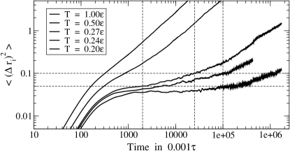
Figure 2: The dependencies of the mean square particles’ displacements on time for five studied temperatures. The data were collected on the system of 5324 particles at the same number density that was used in simulations of the large system.

V Results of Simulations

V.1 Studied system

We studied a system consisting of $50\%$ of particles A and $50\%$ of particles $B$. The particles interact through the pairwise repulsive potential:

$$U_{ab}(r_{ij})=\epsilon\left(\frac{\sigma_{ab}}{r_{ij}}\right)^{12}\;.\;\;\;\;$$ (58)

In (58) $\sigma_{ab}$ is the length that determines the characteristic interaction range. The indices $a$ and $b$ stand for the types of particles: $A$ or $B$. In the following we measure the temperature, $T$, in units of $\epsilon$. Further:

$$\sigma_{AA}=1.0\;,\;\sigma_{BB}=1.2\;,\;\sigma_{AB}=\frac{\sigma_{AA}+\sigma_{BB}}{2}=1.1\;,\;\;\;\;\;\;\;$$ (59)

$$m_{B}=2m_{A}\;,\;\tau=\sqrt{\frac{m_{A}\sigma_{AA}^{2}}{\epsilon}}\;,\;\;N_{A}=N_{B}=31250\;,\;\;\;$$ (60)

$$L_{x}=L_{y}=L_{z}=42.7494\sigma_{AA}\;,\;\;\rho_{o}=0.80/\sigma_{AA}^{3}\;,$$ (61)

where $m_{A}$ and $m_{B}$ are the masses of particles $A$ and $B$. The time unit is $\tau$. $N_{A}$ and $N_{B}$ are the numbers of particles. The lengths of the sides of the cubic simulation box are $L_{x},L_{y},L_{z}$. The number density is $\rho_{o}$. Periodic boundary conditions were used.

This system of particles was extensively studied previously Hansen19881; Miyagawa19911; Mizuno20101; Mizuno20111; Matsuoka2012; Mizuno20131. However, this model was not studied previously from the perspective of atomic level stresses.

We used LAMMPS molecular dynamics (MD) package in our simulations Plimpton1995; lammps. Initial particles’ configuration was created as FCC lattice with alternating planes of $A$ and $B$ particles. The system was melted and equilibrated at temperature $T=2$ in the NVT ensemble. The equilibration was controlled by the absence of change in the average value of potential energy and by the absence of change in the partial pair density functions. Equilibration is achieved when particles are well mixed. Further we reduced the temperature in the NVT ensemble to $T=1.5$ and again equilibrated the system. Then we reduced the temperature to $T=1$. After the equilibration we switched to the NVE ensemle. After the equlibration we collected structural configurations. Similar algorithm was used to collect configurations at temperatures $T=0.5$ and $T=0.27$. We also produced inherent structures by applying conjugate gradient relaxation to the structures (restart files) collected at the temperatures $T=0.27$ and $T=1$.

V.2 Mean square particles’ displacement and the partial pair density correlation functions

Figure 2 shows how the mean square particles’ displacement, msd, depends on time at different temperatures. The msds for Fig.2 were calculated without making the distinction between the particles of type “A” and “B”. The purpose of Fig.2 is to remind about the characteristic temperature scales Hansen19881; Miyagawa19911; Mizuno20101; Mizuno20111; Matsuoka2012; Mizuno20131.

Panels (a,b,c) of Fig.19 show the partial pair density functions, p-pdf-s,  at temperatures $T=1$, $T=0.5$, $T=0.27$, and the p-pdf-s  calculated on the inherent structures. As temperature is reduces from $T=1$ to $T=0.27$ the p-pdf-s  do not show pronounced changes. The famous splitting of the second peak EMa20111; Pan20111 becomes noticeable, but it is not pronounced in comparison with the well expressed splitting observed on the inherent structures. Another thing to notice is that the p-pdf-s  for the pairs of particles of different types exhibit qualitatively similar behaviour at all temperatures. Figure 19 will be useful in the following as it shows the characteristic length scales, such as the positions of the first peak, first minimum, second peak, and the position where the splitting of the second peak occurs. It also will be useful because it shows the amplitudes of the changes on the y-axis on decrease of temperature.

V.3 Distributions of the Atomic Level Stresses

Using formula (4) the Cartesian components of the atomic stress tensor of every atom can be calculated if the atomic configuration is known. Then, using formulas (22,22,22,22) for every atom, the $\sigma_{i}^{sph}$s  of the atomic stress tensors can be obtained. We performed these calculations for several temperatures and obtained the probability distributions (PDs) of the $\sigma_{i}^{sph}$s  by averaging over all relevant atoms and over 100 different configurations for every temperature.

The PDs  of the atomic pressure, $p_{i}\equiv s_{0,i}$, for “A” and “B” particles are shown in panels (a) and (b) of Fig.3. The finite widths of the PDs  of the pressure calculated on inherent structures, i.e., at $T=0$, are caused by the structural disorder only. At non-zero temperatures there are structural and vibrational contributions to the PDs  of the pressure. Since in the studied system particles interact through the purely repulsive potentials the pressure on every atom has to be positive. As temperature increases the average pressure also increases. The widths of the PDs  also increase with increase of temperature.

Panel (b) shows that the average pressure on “B”-particles is larger than the average pressure on “A” particles. Note that, according to the definition (4), the contribution of every neighbour to the diagonal stress tensor components is always positive for the purely repulsive potentials. Therefore the pressure, which is proportional to the sum of the diagonal components, on average becomes proportional to the average number of the neighbours. Thus, since larger atoms on average have more neighbours, they also tend to have larger pressure. These considerations, however, do not take into account the fact that larger atoms also have larger atomic volume. If the difference in the atomic volumes is taken into account then the atoms of both types should have similar values of the pressure. Thus, the discrepancy in the values of the atomic pressure in Fig.3 is caused by the identical values of the atomic volume $\langle V_{i}\rangle$ used for both types of particles in (4).

It is possible to introduce artificially the atomic volume which would account for the difference in sizes between “A” and “B” particles Egami19802; Egami19821; Chen19881; Levashov2008B. This should lead to the similar values of the average atomic pressure for both types of particles. Note that at $T=0.27$ the maximum in the PD  of pressure for “A”-particles occurs at $s_{0,i}^{max}(A)\approx 7$, while for “B”-particles at $s_{0,i}^{max}(B)\approx 10$. Thus $s_{0,i}^{max}(B)/s_{0,i}^{max}(A)\approx 10/7\approx 1.43$. In order to have the same pressure on both types of particles it is necessary to assume that the volume of “B”-particle is $\approx 1.43$ times larger than the volume of “A”-particle. This means that the radius of “B”-particles should be $\approx 1.13$ times larger than the radius of “A”-particles. This result can be compared with (59). In our present considerations we use the same value of $\langle V_{i}\rangle=1/\rho_{o}$ for both types of particles. We prefer do not use the atom-dependent atomic volume because it is not present in the Green-Kubo formula for viscosity Levashov20111; Levashov2013.

The PDs  of the Cartesian components $\sigma_{i}^{xx}$, $\sigma_{i}^{yy}$, and $\sigma_{i}^{zz}$ for “B”-particles at $T=1$ are shown in panel (a) of Fig.12 with the blue curves (these curves coincide into one). The PDs  of the Cartesian components $\sigma_{i}^{xx}$, $\sigma_{i}^{yy}$, and $\sigma_{i}^{zz}$ for “A”-particles at $T=0.27$ are shown in panel (a) of Fig.13 with the blue curves.

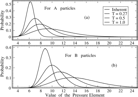
Figure 3: The PDs  of the pressure elements for the particles of type “A” in panel (a) and for the particles of type “B” in panel (b) for different temperatures. The lower the temperature the more pronounced is the peak in the $PD$. At lower temperatures the average pressure is smaller. Thus the peaks corresponding to the lower temperatures are located to the left with respect to the higher temperature peaks.

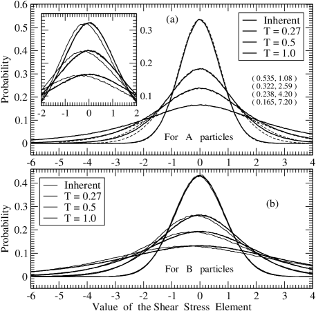
Figure 4: Panel (a): The solid curves in the main plot show the $PDs$ of the $\sigma_{i}^{sph}$s  (except $s_{5,i}$) for “A” particles at different temperatures. See formulas (22,22,22). The lower the temperature the narrower and taller are the corresponding peaks. The dashed curves are the Gaussian functions with which the peaks of the PDs  are fitted. The numbers in brackets show the parameters $a$ and $b$ of the fitting functions: $f(s)=a\exp\left[-(s^{2}/b^{2})\right]$. Since the tails of the PDs  are not well fitted, while the peaks are fitted, it is clear that the PDs  for the $\sigma_{i}^{sph}$s  are not Gaussians. The inset shows the peaks of the PDs  for $\sigma^{xy}_{i}$, $\sigma^{xz}_{i}$, $\sigma^{yz}_{i}$, $\tfrac{1}{2}(\sigma^{xx}_{i}-\sigma^{yy}_{i})$, and $\tfrac{1}{\sqrt{3}}\left[\sigma^{zz}_{i}-\tfrac{1}{2}(\sigma^{xx}_{i}+\sigma^{yy}_{i})\right]$ at the temperatures $T=1.0$, $T=0.5$, and $T=0.27$. Note that the PDs  of $\tfrac{1}{\sqrt{3}}\left[\sigma^{zz}_{i}-\tfrac{1}{2}(\sigma^{xx}_{i}+\sigma^{yy}_{i})\right]$ are noticeably different from the other PDs  . In our view, this difference indicates that different $\sigma_{i}^{sph}$s  are not (completely) independent. Panel (b): The PDs  of the $\sigma_{i}^{sph}$s  at different temperatures for “B” particles. Note that the PDs  of the $\tfrac{1}{\sqrt{3}}\left[\sigma^{zz}_{i}-\tfrac{1}{2}(\sigma^{xx}_{i}+\sigma^{yy}_{i})\right]$ component are noticeably different from the PDs  of the other components. Also note that this difference is nearly absent in the curves obtained from the inherent structures.

Figure 4 shows the PDs  of the shear $\sigma_{i}^{sph}$s  for “A” and “B” particles at different temperatures. The means of these PDs  naturally occur at zero value. The widths of the PDs  calculated on the inherent structures originate from the structural disorder only. As temperature increases the PDs  become wider. At non-zero temperatures there are structural and vibrational contributions to the shear $\sigma_{i}^{sph}$s, as for the pressure. Note that the PDs  for “B” particles are wider than for “A”-particles. They are wider because particles of “B”-type on average have more neighbours than “A”-particles and thus the shear $\sigma_{i}^{sph}$s  for “B”-particles fluctuate in a wider range than the stress components for “A”-particles. This difference can be taken into account by assuming that “A” and “B” particles have different atomic volumes, $\langle V_{i}\rangle$. However, in the present paper we use the same value of the atomic volume in (4). The dashed curves in panel (a) show the Gaussians whose parameters were adjusted to fit the peaks of the PDs  obtained in MD simulations. It is clear that these fits do not match the tails of the PDs  obtained in MD simulations. Thus, the PDs  of the shear stresses are not described well by the Gaussian functions.

The inset in panel (a) of Fig.4 shows that the PDs  of the shear component $(1/\sqrt{3})\left[\sigma_{i}^{zz}-\tfrac{1}{2}\left(\sigma_{i}^{xx}+\sigma_{i}^{yy}\right)\right]$ are noticeably different from the distributions of the other shear stress components. This effect is present for “A” and “B” particles, as follows from the comparison of the inset in panel (a) with the panel (b) itself. We interpret this difference as an indication that different $\sigma_{i}^{sph}$s  are not completely independent from each other. This issue is discussed more in the following.

V.4 Eigenvalues of the atomic stress matrices and correlations between the eigenvalues

The real and symmetric $3\times 3$ matrix of the atomic stress tensor (4) can be diagonalized and its eigenvalues and eigenvectors can be found KoppJ20081. For purely repulsive potentials all eigenvalues should be positive. This can be demonstrated as follows. Let us assume that $\bf{b}$ is an arbitrary column vector, while $\bf{b}^{T}$ is the transpose of $\bf{b}$, i.e., the raw-vector. Let us consider the inner product:

$$\bm{b}^{T}\Sigma_{i}\bm{b} =\sum_{\alpha\beta}b^{\alpha}\sigma_{i}^{\alpha\beta}b^{\beta}=\sum_{\alpha\beta}b^{\alpha}\left(-\sum_{j}\frac{\partial U}{\partial r_{ij}}\frac{r_{ij}^{\alpha}r_{ij}^{\beta}}{r_{ij}}\right)b^{\beta}\;\;\;\;\;\;\;\;$$ (62)

$$=-\sum_{j}\left(\frac{\partial U}{\partial r_{ij}}\right)\frac{\left(\bm{b}\bm{r}_{ij}\right)^{2}}{r_{ij}}\;.\;\;$$

For a purely repulsive potential the derivative of the potential is negative and thus (62) is positive. Thus the atomic stress matrices for the purely repulsive potentials are positive-definite matrices. Let us now assume that vector $\bm{b}$ is not an arbitrary vector, but an eigenvector of the matrix $\Sigma_{i}$. In this case we get: $\bm{b}^{T}\Sigma_{i}\bm{b}=\lambda(\bm{b}\bm{b})=\lambda b^{2}$. The comparison of this result with (62) leads to the conclusion that all eigenvalues, $\lambda$, should be positive.

Thus the atomic stress matrix for every particle has 3 positive eigenvalues $\lambda_{1}$, $\lambda_{2}$, and $\lambda_{3}$ which describe the geometry of the local atomic environment. Further we assume that the eigenvalues are ordered: $\lambda_{1}\geq\lambda_{2}\geq\lambda_{3}$.

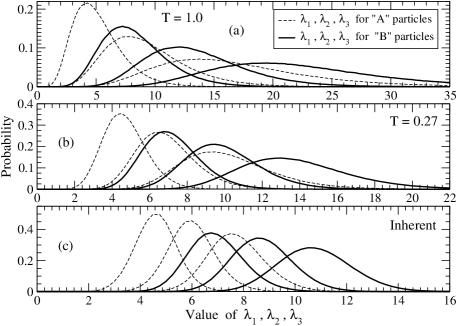
Figure 5: The PDs  of the eigenvalues for particles of type “A” and “B” at temperatures $T=1.0$ (panel (a)), $T=0.27$ (panel (b)), and in the inherent structures obtained from the structures at $T=0.27$ (panel (c)). Note that the scales on the axes in all panels are different. Since, for every particle, $\lambda_{1}\geq\lambda_{2}\geq\lambda_{3}$ the peaks of the PDs  corresponding to the larger eigenvalues are located to the right with respect to the peaks of the curves corresponding to the smaller eigenvalues.

Figure 5 shows the PDs  of the ordered eigenvalues for “A” and “B” particles at different temperatures. As temperature decreases the eigenvalues, in general, become smaller and their PDs  become narrower. This is the expectable behaviour.

Correlations between the eigenvalues of the same atomic stress tensor were studied in Ref.Kust2003a; Kust2003b for several model systems, but not for the system that we study. It was demonstrated that there are correlations between the eigenvalues. However, the real understanding of the nature of these correlations has not been achieved. Thus we decided to elaborate further on these correlations. In particular, we considered the PDs  of the ratios $(\lambda_{2}/\lambda_{1})$  and $(\lambda_{3}/\lambda_{2})$  . These PDs  are shown in Fig.6.

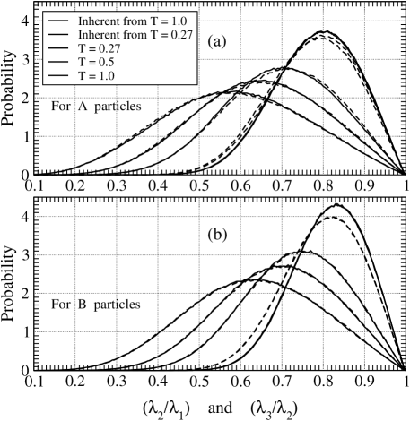
Figure 6: The solid curves in both panels show the PDs  of the ratio $(\lambda_{2}/\lambda_{1})$, while the dashed curves show the PDs  of the ratio $(\lambda_{3}/\lambda_{2})$. Panel (a) shows the results for “A” particles at different temperatures, while panel (b) shows the results for “B” particles. Note from panel (a) that the PDs  of $(\lambda_{2}/\lambda_{1})$  and $(\lambda_{3}/\lambda_{2})$  for the particles of type “A” essentially coincide at all temperatures in the liquid state. On the other hand, in the inherent states, there appears a more noticeable difference in the PDs  of $(\lambda_{2}/\lambda_{1})$  and $(\lambda_{3}/\lambda_{2})$  . In panel (b) the differences in the PDs  of $(\lambda_{2}/\lambda_{1})$  and $(\lambda_{3}/\lambda_{2})$  are even smaller than in panel (a) for the temperatures corresponding to the liquid states. On the other hand, in the inherent states, the difference between the two PDs  becomes quite significant. The coincidence of the PDs  of $(\lambda_{2}/\lambda_{1})$  and $(\lambda_{3}/\lambda_{2})$  is not a trivial point. As we demonstrate further this coincidence is not a general property. Note also that all curves arrive to the point $(\lambda_{2}/\lambda_{1})=(\lambda_{3}/\lambda_{2})=1$ in a linear fashion. See Appendix (LABEL:sec:app-l2overl1).

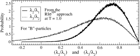
Figure 7: The PDs  of $(\lambda_{2}/\lambda_{1})$  and $(\lambda_{3}/\lambda_{2})$  obtained using the $RI\sigma^{sph}\;$approach for “B” particles at $T=1.0$. Thus, in the random and independent case for the spherical stresses, there is no coincidence in the PDs  of $(\lambda_{2}/\lambda_{1})$  and $(\lambda_{3}/\lambda_{2})$, while both distributions obtained directly from MD simulations are essentially the same, as shown in Fig.6(b).

Note in Fig.6 that the PDs  of $\left(\lambda_{2}/\lambda_{1}\right)$ and $\left(\lambda_{3}/\lambda_{2}\right)$ are very similar to each other for “A” and “B” particles, if the system is in a liquid state. The PDs  of $\left(\lambda_{2}/\lambda_{1}\right)$ and $\left(\lambda_{3}/\lambda_{2}\right)$ for “B”-particles are essentially identical to each other. This finding is not expectable, and, in our view, it is rather surprising. The similarity in these PDs  can not be a general property, as a difference between the PDs  can be observed in the results obtained on the inherent structures. For “A”-particles the difference in the PDs  obtained on the inherent structures is noticeable, while the results for “B”-particles show a very clear difference.

The fact that the coincidence of the PDs  of $(\lambda_{2}/\lambda_{1})$  and $(\lambda_{3}/\lambda_{2})$  is something unusual can also be demonstrated using the $RI\sigma^{sph}\;$approach described in section III. Thus Fig.7 shows the PDs  of $(\lambda_{2}/\lambda_{1})$  and $(\lambda_{3}/\lambda_{2})$  calculated using the $RI\sigma^{sph}\;$approach on the PDs  of the $\sigma_{i}^{sph}$s  corresponding to “B” particles at $T=1$. We see in Fig.7 that the PDs  of $(\lambda_{2}/\lambda_{1})$  and $(\lambda_{3}/\lambda_{2})$  from the $RI\sigma^{sph}\;$approach are completely different, while on MD data, as Fig.6(b) shows, they are simply identical.

In order to get further insight into the PDs  of $\left(\lambda_{2}/\lambda_{1}\right)$ and $\left(\lambda_{3}/\lambda_{2}\right)$ we considered the PD  of the pair of values $\left(\lambda_{2}/\lambda_{1}\right)$ and $\left(\lambda_{3}/\lambda_{2}\right)$. The contour plot of this PD  is shown in Fig.8.

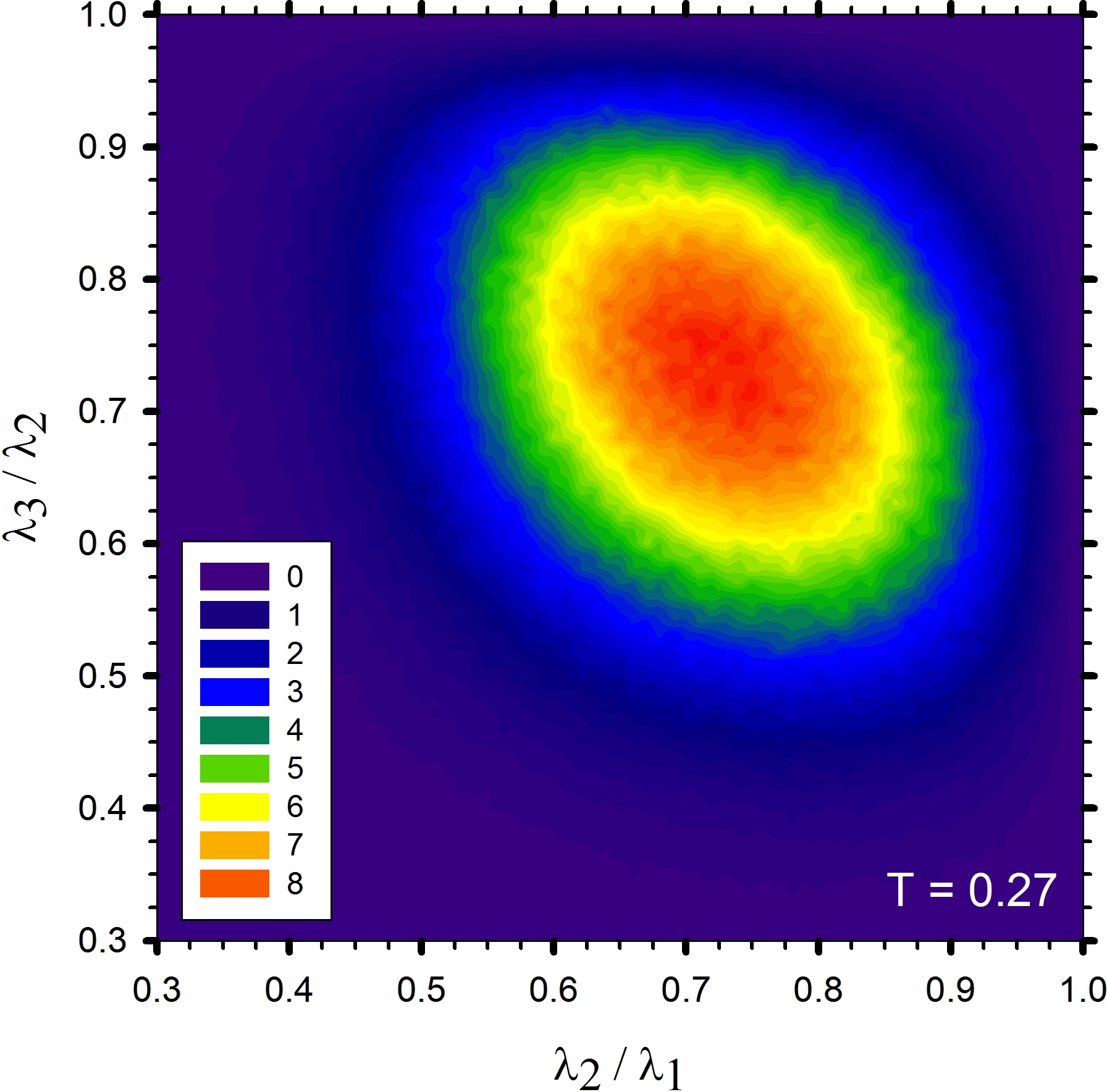
Figure 8: 2D contour plot of the PD  for the ratios of eigenvalues $[(\lambda_{2}/\lambda_{1}),(\lambda_{3}/\lambda_{2})]$ for “A” particles at $T=0.27$. The amplitude of the probability (on $z$-axis) was multiplied by 10000. Note that the distribution appears to be symmetric with respect to the diagonal “$(\lambda_{2}/\lambda_{1})=(\lambda_{3}/\lambda_{2})$”. This point is verified in Fig.9. This means that the probability function $W\left[(\lambda_{2}/\lambda_{1}),(\lambda_{3}/\lambda_{2})\right]$ is symmetric with respect to the interchange of its arguments: $W\left(x_{1},x_{2}\right)=W\left(x_{2},x_{1}\right)$. We observed similarly symmetric distributions for the other temperatures in the liquid states for the particles of both types.

This figure suggests that the probability distribution, $W(\lambda_{2}/\lambda_{1},\lambda_{3}/\lambda_{2})$, of $\left(\lambda_{2}/\lambda_{1}\right)$ and $\left(\lambda_{3}/\lambda_{2}\right)$ is symmetric with respect to the diagonal “$\left(\lambda_{2}/\lambda_{1}\right)=\left(\lambda_{3}/\lambda_{2}\right)$”. This means that $W(x_{1},x_{2})=W(x_{2},x_{1})$. This point is verified in Fig.9 that shows the cuts of $W(\lambda_{2}/\lambda_{1},\lambda_{3}/\lambda_{2})$ along the lines orthogonal to the diagonal “$\left(\lambda_{2}/\lambda_{1}\right)=\left(\lambda_{3}/\lambda_{2}\right)$” at two different temperatures. Because of this symmetry it might be tempting to assume that $W\left(x_{1},x_{2}\right)=W(x_{1})W(x_{2})$. However, we checked this point and found that this last assumption is incorrect.

We verified that the contour plots for the other non-zero temperatures also appear to be symmetric with respect to the diagonal from “South-West” to “North-East”.

Figure 9: The cuts of the PDs, analogous to those in Fig.8, along the lines orthogonal to the diagonal “$(\lambda_{2}/\lambda_{1})=(\lambda_{3}/\lambda_{2})$”. Such lines intersect the diagonal at points $(\xi,\xi)$, where $\xi=(\lambda_{2}/\lambda_{1})=(\lambda_{3}/\lambda_{2})$. The values of $\xi$ for the intersection points are shown as legends in the panels. The legends from top to the bottom correspond to the curves from top to the bottom. The distances from the intersection points along the orthogonal cuts are shown on the $x$-axis. Two curves for every intersection point correspond to the two directions from the diagonal (North-West and South-East). Thus the figure shows that the probability distributions $W\left(x_{1},x_{2}\right)$ are indeed quite symmetric with respect to the interchange of its arguments.

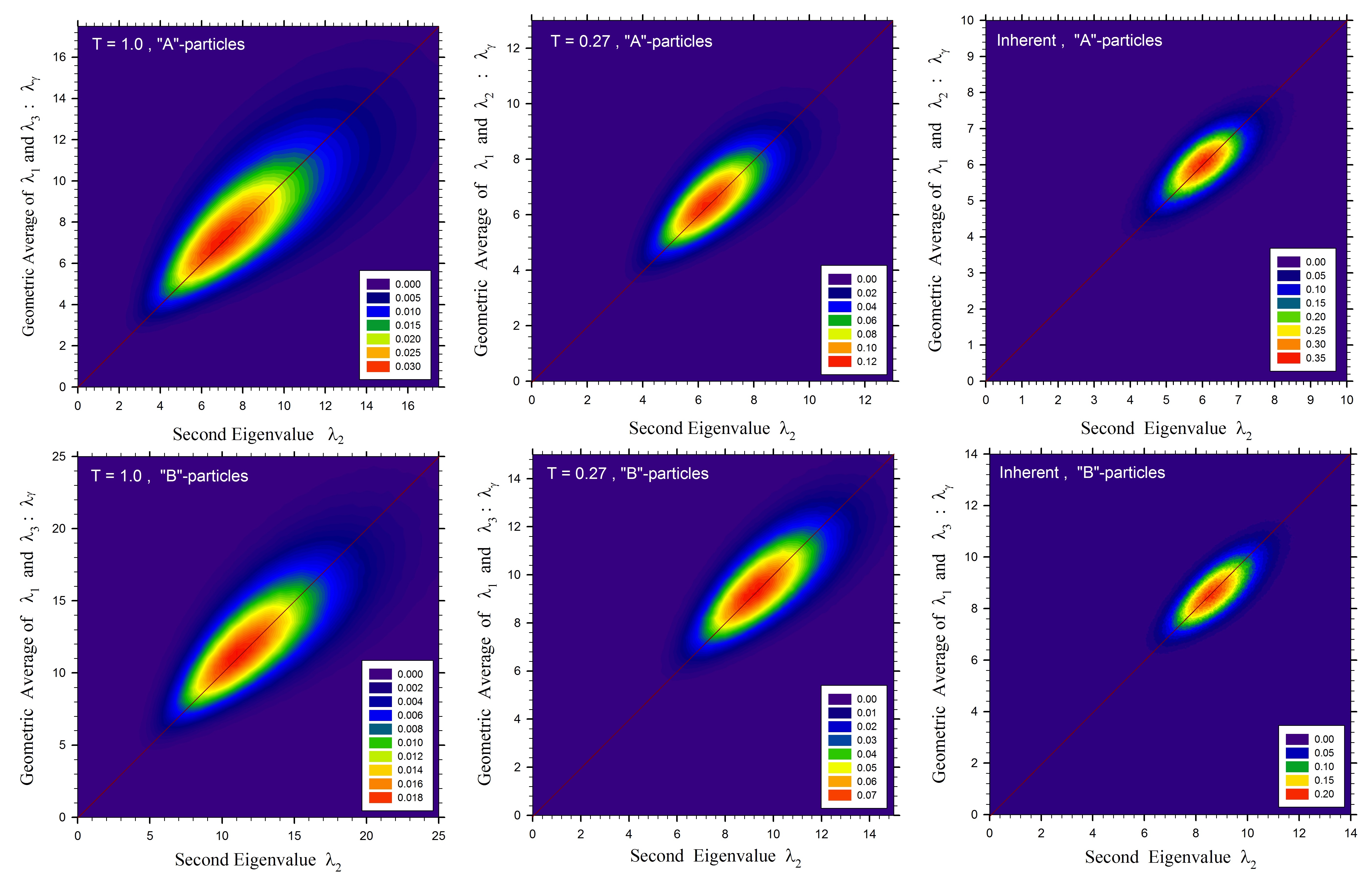
Figure 10: The 2D PDs  for the occurrence of pairs $(\lambda_{2},\sqrt{\lambda_{1}\lambda_{3}})$ for “A” and “B” particles for temperatures $T=1.0$, $T=0.27$, and for the inherent structures obtained from $T=0.27$. The concentration of probability along the diagonal “$\lambda_{2}=\lambda_{geom}$”, as well as the symmetry of the PDs  with respect to this diagonal, suggest that indeed $\lambda_{2}$ tends to be $\sqrt{\lambda_{1}\lambda_{3}}$.

The observed symmetry with respect to the diagonal “$(\lambda_{2}/\lambda_{1})=(\lambda_{3}/\lambda_{2})$” lead us to think that $\lambda_{2}$ tends to be the geometric average of $\lambda_{1}$ and $\lambda_{3}$. Indeed, if $\lambda_{2}=\sqrt{\lambda_{1}\lambda_{3}}$ then $(\lambda_{2}/\lambda_{1})=(\lambda_{3}/\lambda_{2})$.

In order to verify the assumption that $\lambda_{2}$ tends to be the geometric average of $\lambda_{1}$ and $\lambda_{3}$ we calculated the 2D contour plots of the PDs  of the occurrence of pairs $(\lambda_{2},\lambda_{geom})$, where $\lambda_{geom}\equiv\lambda_{\gamma}\equiv\sqrt{\lambda_{1}\lambda_{3}}$. These plots for “A” and “B” particles for temperatures $T=1.0$, $T=0.27$, and for the inherent structures (produced from the configurations at $T=0.27$) are shown in Fig.10. It follows from Fig.10 that the maximums of the PDs  indeed occur at $\lambda_{2}\approx\lambda_{geom}$. Note also the symmetry of the PDs  with respect to the diagonal “$\lambda_{2}=\lambda_{geom}$”.

It is possible also to ask the following question. Is the geometric average of $\lambda_{1}$ and $\lambda_{3}$, as an approximation for $\lambda_{2}$, is much better than the arithmetic average of $\lambda_{1}$ and $\lambda_{3}$? The answer to this question follows from the comparison of the upper four panels in Fig.11. Thus $\sqrt{\lambda_{1}\lambda_{3}}$ is indeed a better approximation for $\lambda_{2}$ than $\tfrac{1}{2}(\lambda_{1}+\lambda_{3})$.

In the considerations of correlations between the eigenvalues it is of interest to understand the scale of the existing correlations. We used $RI\sigma^{sph}\;$approach described in section III in order to estimate the effect of correlations between the $\sigma_{i}^{sph}$s  on the PDs  presented in Fig.11.

We proceeded as follows. Using the PDs  of the $\sigma_{i}^{sph}$s  obtained in MD simulations, we generated the atomic pressure and five atomic $\sigma_{i}^{sph}$s  with the random number generator, as described in section III. Thus, all six $\sigma_{i}^{sph}$s  were generated independently. Then, using these six numbers and formulas (23,24,25,26), we produced six Cartesian stress components, i.e., the Cartesian stress matrix. Then, by diagonalising this stress matrix, we produced three eigenvalues. Then we calculated the geometric average of the largest and the smallest eigenvalues. The lower two panels in Fig.11 show the probability distributions for the pairs $(\lambda_{2},\sqrt{\lambda_{1}\lambda_{3}})$ obtained by means of this random generation procedure. The comparison of the upper two panels in Fig.11 with the lower two panels suggests the presence of correlations between the $\sigma_{i}^{sph}$s.

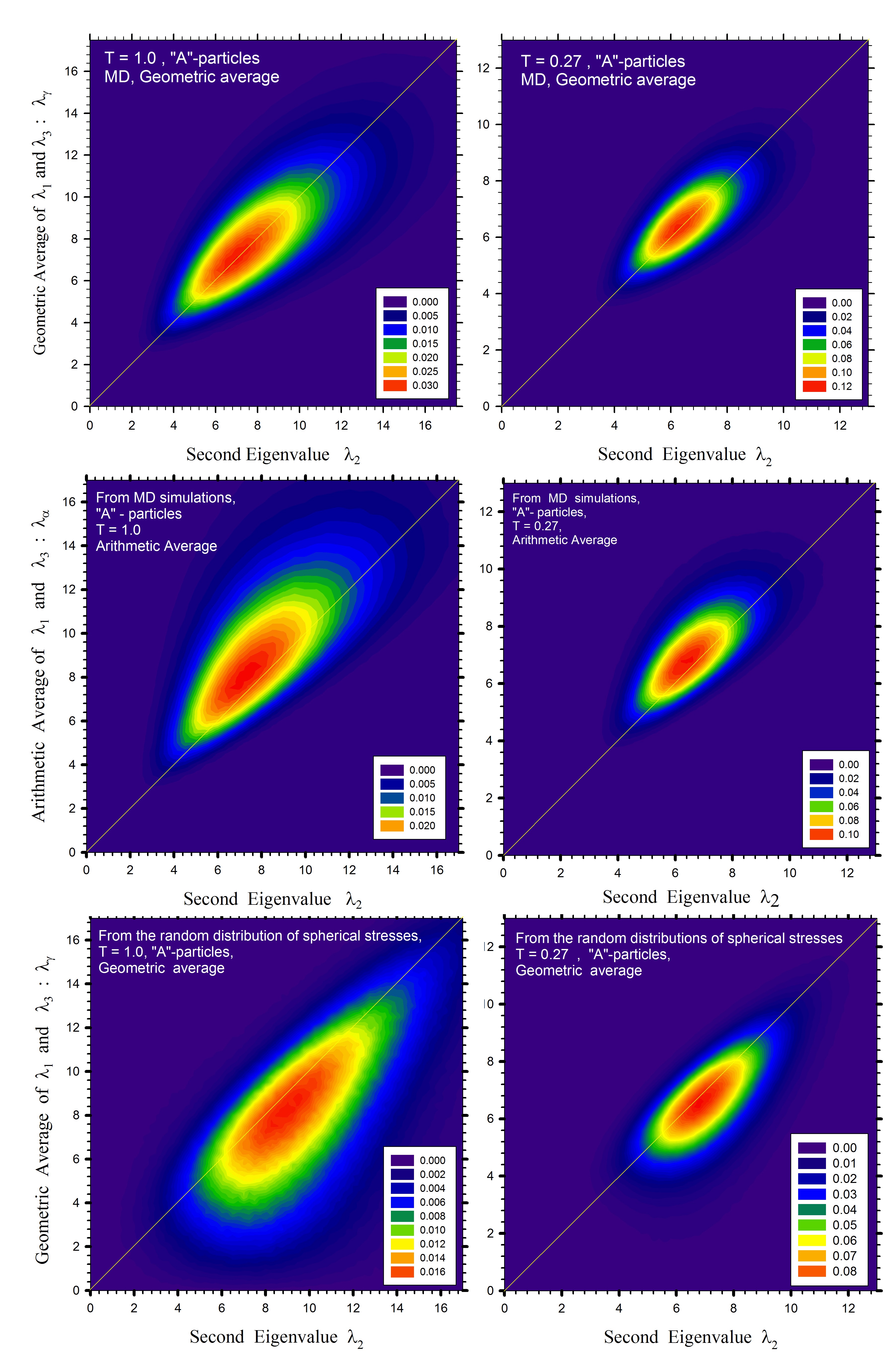
Figure 11: The top two panels show the 2D PDs  of $\lambda_{2,i}$ and the geometric average of $\lambda_{1,i}$ and $\lambda_{3,i}$, i.e., $\lambda_{\gamma,i}\equiv\sqrt{\lambda_{1,i}\lambda_{3,i}}$, at temperatures $T=1.0$ and $T=0.27$ obtained directly from the MD configurations. Thus the top two panels show how good is $\lambda_{\gamma,i}$ as an approximation for $\lambda_{2,i}$. In the middle two panels the arithmetic average, $\lambda_{\alpha,i}=(1/2)(\lambda_{1,i}+\lambda_{2,i})$, was used instead of $\lambda_{\gamma,i}$. The comparison of the top and middle panels shows that $\lambda_{\gamma,i}$ is a better approximation for $\lambda_{2,i}$ than $\lambda_{\alpha,i}$. The bottom two panels show the PDs  for $\lambda_{2,i}$ and $\lambda_{\gamma,i}$ obtained using the $RI\sigma^{sph}\;$approach. The comparison of the top two panels with the bottom two panels shows that the results obtained directly from MD simulations and from the $RI\sigma^{sph}\;$approach are quite different. This demonstrate the presence of correlations between the $\sigma_{i}^{sph}$s.

In order to measure the magnitude of the correlations we calculated quantities,

$$\gamma=\left<\tfrac{\sqrt{(\lambda_{geom,i}-\lambda_{2,i})^{2}}}{\lambda_{2,i}}\right>_{i},\;\;\;\alpha=\left<\tfrac{\sqrt{(\lambda_{arith,i}-\lambda_{2,i})^{2}}}{\lambda_{2,i}}\right>_{i}.\;\;\;\;\;\;\;$$ (63)

which show how well the geometric and arithmetic averages of $\lambda_{1}$ and $\lambda_{3}$ approximate $\lambda_{2}$. We calculated these quantities using the eigenvalues obtained directly from MD simulations. We also calculated $\gamma$ from (63) using the $RI\sigma^{sph}\;$approach described in section III. The results of the calculations are presented in Table (1).

Table 1: The values of $\gamma$ and $\alpha$ from (63) for “A” and “B” particles at different temperatures.

Calculated quantity	T = 1.0	T = 0.5	T = 0.27	T = 0
$\gamma$ for “A”-MD	0.20	0.16	0.13	0.09
$\alpha$ for “A”-MD	0.303	0.211	0.157	0.09
$\gamma$ for “A”-$RI\sigma^{sph}\;$	0.301	—	0.156	—
$\gamma$ for “B”-MD	0.17	0.13	0.11	0.07
$\alpha$ for “B”-MD	0.228	0.162	0.125	0.08
$\gamma$ for “B”-$RI\sigma^{sph}\;$	0.229	—	—	—

It follows from Table (1) that the geometric average, i.e., $\sqrt{\lambda_{1}\lambda_{3}}$, approximation to $\lambda_{2}$ is noticeably better than the arithmetic average on the data obtained from MD simulations. It also follows from the table that the geometric average from the $RI\sigma^{sph}\;$approach is approximately as good as the arithmetic average from MD simulations.

As we demonstrated that there are correlations between the eigenvalues of the atomic stress tensors there arises the question about the importance of these correlations from the macroscopic perspective. In our view, the observed correlations between the eigenvalues can be related to the atomistic origin of the Poisson ratio (effect). Thus, for macroscopic samples elongation in one direction usually leads to contraction in the directions orthogonal to the direction of elongation. The magnitude of this effect is determined by the Poisson ratio. Thus, for a given sample, there is a correlation between its length and its width. In our view, this effect can originate from the correlations between the eigenvalues of the atomic stresses.

V.5 Correlations between the eigenvalues and the random and independent approximations

In the previous subsection we demonstrated that there are correlations between the eigenvalues of the atomic stress tensors. We also speculated that these correlations might be related to the Poisson ratio effect. Thus it is important to gain a better understanding of the correlations between the eigenvalues. Therefore in this subsection we further elaborate on this issue.

In particular, it is of interest to study correlations between the eigenvalues from the following perspective. In the previous considerations of the atomic stresses it was assumed that 6 components of the atomic stress tensor in the spherical representation are independent Egami19821; Chen19881; Levashov2008B in the linear approximation. This assumption allows to introduce the concept of the atomic stress energies and rationalize the values of these energies Egami19821; Chen19881; Levashov2008B. In particular, it was argued that every atom in the liquid with its nearest neighbour shell (in the linear approximation) is equivalent to a 3-dimensional harmonic oscillator Egami19821; Chen19881; Levashov2008B. Further, it was assumed that the potential energy of this oscillator is equally divided between 6 independent atomic stress components. This assumption is supported by the result from MD simulations. Thus, in MD simulations the potential energy of every spherical stress component can be calculated independently and it was demonstrated that the potential energy of every component depends on temperature as “$\tfrac{1}{6}\cdot 3\cdot\tfrac{1}{2}k_{B}T=\tfrac{1}{4}k_{B}T$”.

It follows from the previous paragraph that the assumption about independence of $\sigma_{i}^{sph}$s  plays an important role in the considerations based on the concept of atomic level stresses. Thus, it is reasonable to address the issue of independence of the $\sigma_{i}^{sph}$s. In the following we consider several examples that provide certain insights in the relevant correlations and into their magnitudes.

V.5.1 From Independent and Random Spherical Stress Components to the Cartesian Stress Components and Eigenvalues

As we already discussed, the PDs  of the $\sigma_{i}^{sph}$s  can be obtained from the atomic configurations that were generated in MD simulations. Figures 3,4 provide the examples of such distributions. Using these PDs  random and independent $\sigma_{i}^{sph}$s  can be generated. It is important that generated in this way $\sigma_{i}^{sph}$s  are independent from each other.

Then, using formulas (23,24,25,26), these random and independent $\sigma_{i}^{sph}$s  can be transformed into the Cartesian stress components. After that, the eigenvalues of the obtained stress tensor in the Cartesian representation can also be calculated.

Thus, the PDs  of the Cartesian stress components generated using the described $RI\sigma^{sph}\;$approach can be compared with the PDs  of the Cartesian stress components obtained directly from MD simulations. These comparisons are presented in Fig.12(a),13(a). These figures clearly suggest the presence of correlation between the $\sigma_{i}^{sph}$s. They also demonstrate the scale of the influence of these correlations on the distributions of the Cartesian stress components.

The PDs  of the eigenvalues obtained via the $RI\sigma^{sph}\;$approach also can be compared to the PDs  of the eigenvalues obtained directly from the MD data. Figures 12(b),13(b) show that the PDs  of the eigenvalues obtained directly from MD simulations are quite different from the PDs  obtained via the $RI\sigma^{sph}\;$approach. Thus, while in certain situations the $RI\sigma^{sph}\;$might lead to the reasonable results, it is clear that, after all, it is just an approximation.

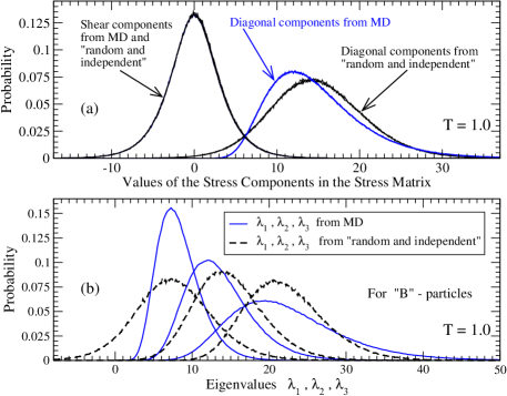
Figure 12: Panel (a) shows the PDs  of the Cartesian stress elements for “B” particles obtained directly from MD simulations and from the $RI\sigma^{sph}\;$approach. There is a perfect agreement between the PDs  for the off-diagonal stress elements. This agreement is not surprising – it is expectable from the relations (22,26) between the spherical and Cartesian stress elements. The disagreement between the PDs  of the diagonal components suggests that the atomic stress components of the same atom are not independent. Panel (b) shows the PDs  of the eigenvalues obtained directly from MD simulations and from the $RI\sigma^{sph}\;$approach. It is clear that the PDs  obtained through these two methods are completely different. This again suggests the presence of correlations between the $\sigma_{i}^{sph}$s  of the same atom and also the presence of correlations between the eigenvalues. Note that the eigenvalues from MD simulations are always positive, while the eigenvalues from the $RI\sigma^{sph}\;$approach can be negative.

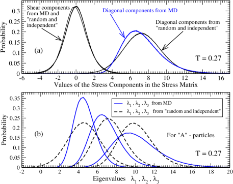
Figure 13: Similar to Fig.12, but for “A” particles at $T=0.27$.

As we already discussed, the geometry of the atomic environment can be describe by six $\sigma_{i}^{sph}$s. However, these six components also describe the orientation of the atomic environment with respect to the reference coordinate frame. If this orientation is irrelevant then the geometry of the atomic environment is described by only 3 numbers, i.e., by eigenvalues. The relation between the PDs  for the eigenvalues and the PDs  for the $\sigma_{i}^{sph}$s  is actually counter-intuitive. Naively, one can expect that independent PDs  for the eigenvalues should lead to the independent PDs  for the $\sigma_{i}^{sph}$s  and vice versa. However, this is not the case. Thus, in Appendix (LABEL:sec:eigen-to-spherical) we consider an example that demonstrates how independent PDs  for the eigenvalues lead to dependent PDs  for the spherical stresses. Vice versa in Appendix (LABEL:sec:spherical-to-eigen) we show how independent probability distributions for the $\sigma_{i}^{sph}$s  lead to dependent PDs  for the eigenvalues.

V.5.2 Random Distributions of Eigenvalues vs. the Distributions of Eigenvalues from MD Simulations

We used the $RI\lambda\;$approach described in section III in order to generate the PDs  of the three random and independent magnitude-ordered eigenvalues which can be compared to the PDs  of the three magnitude-ordered eigenvalues obtained directly from MD simulations. The results of this procedure are shown in Fig.14.

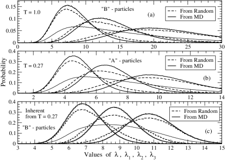
Figure 14: The PDs  of $\lambda_{1},\;\lambda_{2},\;\lambda_{3}$ from MD simulations and from the selection of three eigenvalues from the total random distribution of eigenvalues ($RI\lambda\;$approach). The thin solid curves in all panels show the total PDs  for all eigenvalues irrespective of their magnitudes. The thick solid curves in all panels show the PDs  for $\lambda_{1},\;\lambda_{2},\;\lambda_{3}$ obtained from MD simulations. The dashed curves show the PDs  for the randomly and independently generated $\lambda_{1}^{r},\;\lambda_{2}^{r},\;\lambda_{3}^{r}$. It is clear that the distributions obtained from MD simulations are noticeably different from the distributions obtained from the “random” approach. This again suggests the presence of correlations between the eigenvalues.

It is also of interest to consider the distributions of the stress tensor invariants obtained directly from MD simulations and also by means of the $RI\lambda\;$approach. The results are presented in Fig.15.

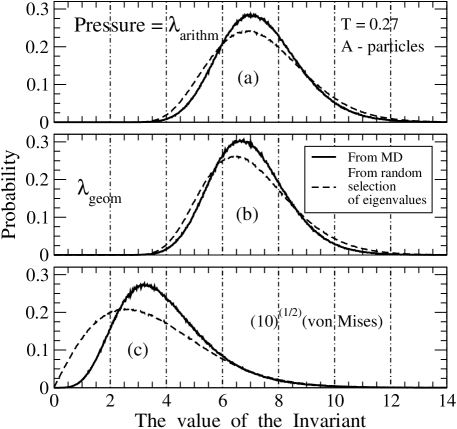
Figure 15: The PDs  of the stress tensor invariants for “A”-particles at $T=0.27$. The solid lines in all panels show the results obtained from MD simulations, i.e., by diagonalization of the atomic stress matrices. The dashed curves in all panels show the PDs  of the invariants obtained using the $RI\lambda\;$approach. The (a)-panel shows the PDs  for the pressure, i.e., for the arithmetic average of the eigenvalues. The (b) panel shows the PDs  for the geometric average of the eigenvalues $\lambda_{geom}=\left(\lambda_{1}\lambda_{2}\lambda_{3}\right)^{1/3}$. The (c) panel shows the PDs  for the scaled value of the von Mises shear stress: $\left[\left((\lambda_{1}-\lambda_{2})^{2}+(\lambda_{1}-\lambda_{3})^{2}+(\lambda_{2}-\lambda_{3})^{2}\right)/3\right]^{(1/2)}$. All panels suggest the presence of correlations between the eigenvalues of the same atomic stress tensor and demonstrate how these correlations affect the PDs  of the atomic stress tensor invariants.

It follows from Fig.15(a,b) that the PDs  of the local atomic pressure and the cubic root from the “volume” of the stress tensor ellipsoids generated in two ways are clearly different. This difference however is not very large. On the other hand, the PDs  of the scaled square roots from the von Mises shear stresses generated in two ways show more significant difference. Note, in particular, different behaviours of the two distributions in the region of zero von Mises stress. Thus von Mises stresses calculated from the MD data avoid being zero more strongly than the von Mises stresses obtained from the $RI\lambda\;$approach. This means, as we discuss in more details in the following, that the eigenvalues obtained from MD simulations avoid being equal, while there is no (there should not be) such behaviour in the randomly generated eigenvalues.

Figure 16 shows the PDs  of the von Mises stresses for “A” and “B” particles at temperatures $T=1.0$ and $T=0.27$ calculated in three different ways. First, there are the PDs  obtained directly from MD simulations. It follows from these curves that from a qualitative perspective the results for both types of particles are similar. Then there are curves produced by $RI\lambda\;$and $RI\sigma^{sph}\;$approaches described in section III. The curves produced by the $RI\sigma^{sph}\;$approach are of particular interest because they behave near zero value of the von Mises stress in a way similar to the curves obtained from MD simulations. Thus random generation of the $\sigma_{i}^{sph}$s  preserves the repulsion between the eigenvalues.

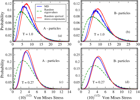
Figure 16: The PDs  of the von Mises stresses for “A” and “B” particles at $T=1.0$ and $T=0.27$. The blue curves in each panel show the results from MD simulations. The results from the $RI\lambda\;$approach are shown with the dashed green curves. The results from the $RI\sigma^{sph}\;$approach are shown with the red curves. Note that the results from the $RI\lambda\;$approach are always quite different from the results of MD simulations. This suggests the presence of correlations between the eigenvalues. On the other hand, the results from the $RI\sigma^{sph}\;$approach are relatively close to the results of MD simulations.

In order to address the correlations between $\lambda_{1}$, $\lambda_{2}$, and $\lambda_{3}$ of the same atomic stress tensor we also considered, as it is usually done, the averaged products $\langle\lambda_{1}\lambda_{2}\rangle$, $\langle\lambda_{1}\lambda_{3}\rangle$, $\langle\lambda_{2}\lambda_{3}\rangle$. It is necessary to realize that the distributions of $\lambda_{1}$, $\lambda_{2}$, $\lambda_{3}$ are not independent by definition. This is because of the convention that for every atomic stress tensor $\lambda_{1}\geq\lambda_{2}\geq\lambda_{3}$. Thus, in order to obtain $\lambda_{1}$, $\lambda_{2}$, and $\lambda_{3}$ three eigenvalues of every atomic stress tensor should be ordered according to their magnitudes. This ordering procedure makes $\lambda_{1}$, $\lambda_{2}$, and $\lambda_{3}$ dependent on each other. We also evaluated $\langle\lambda_{1}\lambda_{2}\rangle$, $\langle\lambda_{1}\lambda_{3}\rangle$, and $\langle\lambda_{2}\lambda_{3}\rangle$ within the $RI\lambda\;$approach. The results of the described calculation are presented in Table 2. It follows from these data that the differences between the averages obtained directly from MD and the averages obtained using the $RI\lambda\;$approach are very small. This demonstrates, in our view, that the most traditional approach to study correlations between two quantities does not really work for the eigenvalues of the atomic stress tensors.

Table 2: The values of the correlators, $\langle\lambda_{1}\lambda_{2}\rangle$, $\langle\lambda_{1}\lambda_{3}\rangle$, $\langle\lambda_{2}\lambda_{3}\rangle$, between the eigenvalues calculated directly from the MD structures and by means of the $RI\lambda\;$approach. Note that the values of the correlators obtained in these two ways are very similar. This suggests that the considered correlators are not sensitive to the existing correlations between the eigenvalues.

Method	$\langle\lambda_{1}\lambda_{2}\rangle$	$\langle\lambda_{1}\lambda_{3}\rangle$	$\langle\lambda_{2}\lambda_{3}\rangle$
MD for “A” at $T=0.27$	74.34	50.79	34.90
$RI\lambda\;$for “A” at $T=0.27$	72.84	51.41	37.63
MD for “B” at $T=1.0$	325.6	198.2	123.1
$RI\lambda\;$for “B” at $T=1.0$	321.8	202.6	135.7
MD for “B” at $T=0$	97.8	77.9	63.4
$RI\lambda\;$for “B” at $T=0$	95.3	77.8	65.1

V.5.3 The Distributions of the Spacings Between the Eigenvalues

In considerations of the eigenvalues’ spectra of the random matrices it is common to consider the distributions of the spacings between the eigenvalues randommatrices; Wigner1967. We also performed this analysis.

The panels (a,b,c) of Fig.17 show the PDs  of the spacings between the eigenvalues for “B”-particles at $T=1.0$. The blue curves were obtained directly from the MD data. The red curves were obtained using the $RI\lambda\;$approach. Zero probability at zero spacing, observed in panels (a,b) in the MD data, suggests that atomic stress tensors avoid having two eigenvalues of the same magnitude. It is likely that this effect originates from the vanishing volume of the phase space associated with the corresponding values of the $\sigma_{i}^{sph}$s  randommatrices. Thus, due to purely probabilistic reason, there essentially no atoms whose environment is almost spherical from the perspective of atomic stresses. Such spherical environments would lead to three eigenvalues which are all equal to each other. However, the data presented in Fig.17 suggest that this essentially never happens.

The red curves in panels (a,b,c) show the PDs  obtained using the $RI\lambda\;$approach. In panels (a) and (b) which correspond to the neighbour eigenvalues there is no “repulsion” between them. This result is expectable for the randomly selected eigenvalues. On the other hand, panel (c) shows “repulsion” between the randomly selected $\lambda_{1}$ and $\lambda_{3}$. It is easy to realize that the “repulsion” between the non-neighbouring eigenvalues has a trivial probabilistic origin. The panels (d,e,f) of Fig.17 show the results for “A”-particles at $T=0.27$. From a qualitative perspective the PDs  for “A”-particles are rather similar to the PDs  for “B”-particles. Note also by comparing panels (a) with (b) and (d) with (e) that the PDs  of $(\lambda_{1}-\lambda_{2})$ are wider than the PDs  of $(\lambda_{2}-\lambda_{3})$.

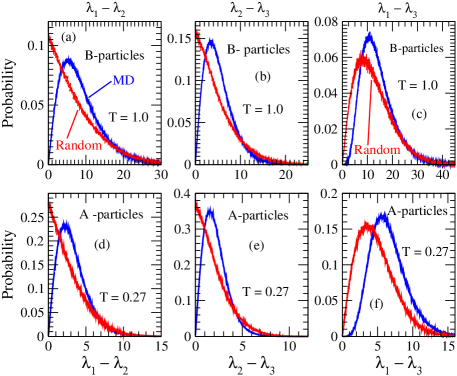
Figure 17: The blue curves in all panels show the PDs  of the spacings $(\lambda_{1}-\lambda_{2})$, $(\lambda_{2}-\lambda_{3})$, $(\lambda_{1}-\lambda_{3})$ obtained directly from MD simulations. The red curves in all panels show the PDs  of the spacings obtained using the $RI\lambda\;$approach. Panels (a,b,c) show the results for “B”-particles at temperature $T=1.0$. Panels (d,e,f) show the results for “A”-particles at temperature $T=0.27$. The curves obtained from MD simulations suggest that local atomic configurations with equal eigenvalues essentially never happen. This follows from the observation that the PDs  from MD go to zero, as spacings $(\lambda_{1}-\lambda_{2})$ and $(\lambda_{2}-\lambda_{3})$ go to zero. The curves obtained using the $RI\lambda\;$approach, in contrast, have maximums at zero values of the spacings. It is easy to realise that the results from the $RI\lambda\;$approach are not surprising.

We also calculated the PDs  of the spacings between the eigenvalues using the $RI\sigma^{sph}\;$approach. The corresponding PDs  are presented in Fig.18. Again note that in MD data in both panels the PDs  of $(\lambda_{1}-\lambda_{2})$ are wider than the PDs  of $(\lambda_{2}-\lambda_{3})$. On the other hand, the PDs  of $(\lambda_{1}-\lambda_{2})$ and of $(\lambda_{2}-\lambda_{3})$ obtained using the $RI\sigma^{sph}\;$approach are identical to each other. Thus there are two red curves in panel (a), i.e., one red curve in panel (a) is the PD  of $(\lambda_{1}-\lambda_{2})$ while another red curve is the PD  of $(\lambda_{2}-\lambda_{3})$. Both curves coincide. The situation is similar for the panel (b).

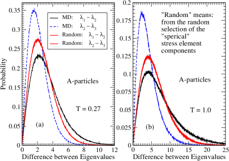
Figure 18: The PDs  of the spacings between the eigenvalues obtained in MD simulations and using the $RI\sigma^{sph}\;$approach. The legends for the curves in both panels are the same. The black curves in both panels show the results for the PDs  of $(\lambda_{1}-\lambda_{2})$ from MD simulations, while blue curves show the PDs  of $(\lambda_{2}-\lambda_{3})$ also from MD simulations. The PDs  for $(\lambda_{1}-\lambda_{2})$ and $(\lambda_{2}-\lambda_{3})$ obtained using the $RI\sigma^{sph}\;$approach coincide, i.e., there are two red curves in each red curve. The PDs  of $(\lambda_{1}-\lambda_{2})$ and of $(\lambda_{2}-\lambda_{3})$ from the $RI\sigma^{sph}\;$approach coincide at $T=0.27$ and at $T=1.0$.

Finally we calculated the average values of the spacings between the eigenvalues using the data from MD simulations, using the $RI\lambda\;$approach, and using the $RI\sigma^{sph}\;$approach. The results are presented in table 3. Note that in MD data $\langle\lambda_{1}-\lambda_{2}\rangle>\langle\lambda_{2}-\lambda_{3}\rangle$. Also note that in the $RI\sigma^{sph}\;$approach $\langle\lambda_{1}-\lambda_{2}\rangle\approx\langle\lambda_{2}-\lambda_{3}\rangle$. It is of interest also that $\langle\lambda_{1}-\lambda_{3}\rangle$ is the same for the MD data and for the $RI\sigma^{sph}\;$approach. On the other hand, $\langle\lambda_{1}-\lambda_{3}\rangle$ in the $RI\lambda\;$approach is smaller than in the other two approaches.

Table 3: The average spacings between the eigenvalues for “A”-particles at $T=0.27$.

Method	$\langle\lambda_{1}-\lambda_{2}\rangle$	$\langle\lambda_{2}-\lambda_{3}\rangle$	$\langle\lambda_{1}-\lambda_{3}\rangle$
MD	3.3	2.2	5.5
$RI\sigma^{sph}\;$	2.8	2.8	5.5
$RI\lambda\;$	2.8	2.0	4.8

VI Correlation Functions Between Different Atoms

In this section we describe the results of our analysis of atomic stress correlations between different atoms. In this analysis, it is natural to compare the results for the stress correlation functions with the results for the partial pair density functions. In particular, it is useful to compare the positions of the characteristic features and also the relative changes in both types of functions on decrease of temperature.

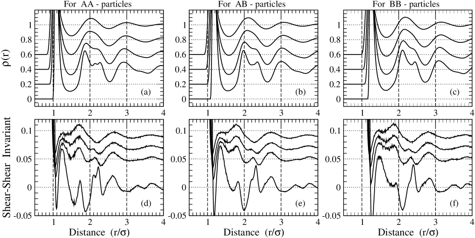
Figure 19: Panels (a,b,c) show the partial pair density functions, $\rho(r)$, for temperatures (from top to the bottom) $T=1.0$, $T=0.5$, $T=0.27$, and $T=0$. The curves for $T=1.0$, $T=0.5$, and $T=0.27$ were shifted upward by 0.6, 0.4, and 0.2 correspondingly. The “inherent” $T=0$ curve was not shifted. Panels (d,e,f) show the invariant shear-shear correlation functions per pair of atoms, defined by formulas (51,52,53,54,56), normalized to the average square of the spherical shear stress component, i.e., $\langle\left(\sigma_{i}^{xy}\right)^{2}\rangle$. The curves for the invariant shear-shear correlation functions at temperatures $T=1.0$, $T=0.5$, and $T=0.27$ were shifted upward by 0.09, 0.07, and 0.05 correspondingly. The “inherent” curve was not shifted. The curves in panels (d,e,f) show how the average correlation state for the pairs of atoms depends on distance and temperature.

VI.1 Partial pair density functions and the stress-stress correlation function invariants related to viscosity

Panels (a,b,c) of Fig.19 show the partial pair density functions for “AA”, “AB”, and “BB”-particles at different temperatures. In each panel the curves from the top to the bottom correspond to the temperatures $T=1.0$, $T=0.5$, $T=0.27$, and $T=0$. The $T=0$ curves were calculated using the inherent structures produced by the conjugate gradient relaxation of the structures at $T=0.27$. The results for the pairs of particles of different types are similar from a qualitative point of view. Since the particles of type “B” are larger than the particles of type “A”, the curves corresponding to the “AB” pairs [see panel (b)] are shifted to the right with respect to the curves corresponding to the “AA” pairs [see panel (a)]. Similarly the curves corresponding to the “BB”-particles [see panel (c)] are shifted to the right with respect to the curves corresponding to the “AB”-particles. As the temperature of the liquid is reduced there appears in all partial pair density curves a noticeable precursor of the famous EMa20111; amorhpous2001; Pan20111 splitting of the second peak. This splitting becomes well pronounced in the $T=0$ state. Overall, the changes in the partial pair density functions (beyond the first peak) observed on decrease of temperature are not very pronounced.

Panels (d,e,f) of Fig.19 show the shear invariant stress correlation function given by formulas (51,52,53,54,56) normalized to the average square of the spherical shear stress component, i.e., to $\langle\left(\sigma_{i}^{xy}\right)^{2}\rangle$. All curves were calculated using the expressions (51,52,53,54). However, we checked that formula (56) leads to the same results.

Note that while the results for the stress correlation functions are presented next to the results for the partial pair density functions the meaning of the stress correlation function curves is quite different. Thus the value of a stress correlation curve at distance $r$ describes the average correlation state of two particles separated by distance $r$.

Note that on decrease of temperature the changes in the stress correlation curves are significantly more pronounced than the changes in the partial pair density curves. In particular, as temperature changes from $T=0.27$ to $T=0$, there is a very abrupt change. Thus the invariant stress correlation function turns out to be quite sensitive to the structural changes that happen to the liquid as it goes into an inherent state. Also note that the range of this abrupt change is limited to the third nearest neighbours. In our view, this means that the stress correlation function is sensitive to the widely discussed formation of the intermediate range order (It is known that the pair density function is not sensitive to the formation of the intermediate range order) MaE20061; EMa20111; Tanaka20131. In our view, the most abrupt changes in the stress correlation functions (in the stress correlation state) happen for (the pairs of atoms separated by) the distance which approximately corresponds to the first minimum in the pair density function. This indicates, in our view, formation of a definite correlated state for weakly connected atoms.

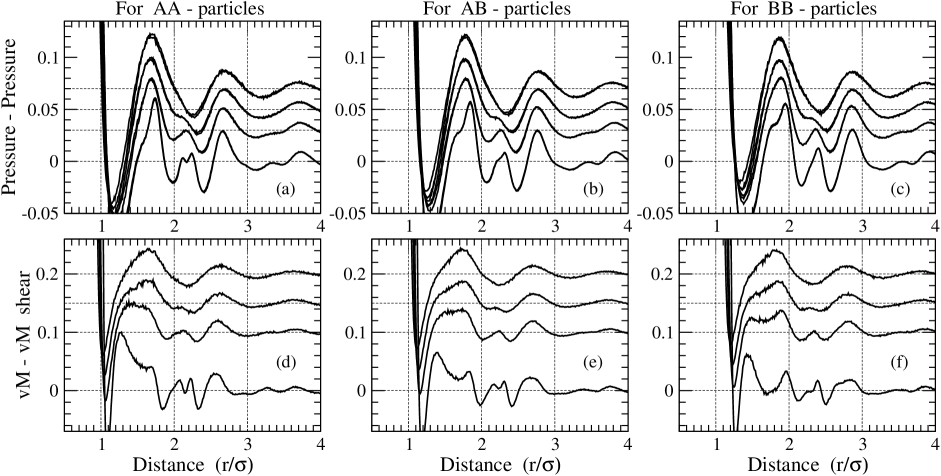
Figure 20: Panels (a,b,c) show the normalized correlation functions between the pressure-pressure invariants. See the first formula in (64). The same panels also show the correlation functions between the third stress tensor invariants, i.e., between the geometric averages of the stress tensor eigenvalues. See the second formula in (64). For the pairs of particles of the same type and at the same temperature these two correlation functions essentially coincide. For this reason every curve in panels (a,b,c) consists of two curves corresponding to two different correlation functions. In all panels in this figure the curves from top to the bottom correspond to the temperatures $T=1.0$, $T=0.5$, $T=0.27$, and $T=0$. Panels (d,e,f) show the normalized (von Mises stress)–(von Mises stress) correlation functions.

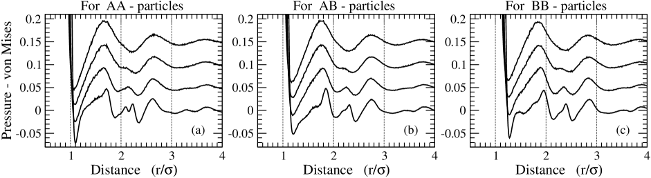
Figure 21: The normalized correlation functions between the pressure and the von Mises stress invariant, i.e., $\left(\langle p_{i}s_{vM,j}\rangle/\langle p_{i}\rangle\langle s_{vM,j}\rangle\right)-1$. In all panels the curves from the top to the bottom correspond to the temperatures $T=1.0$, $T=0.5$, $T=0.27$, and $T=0$.

Panels (a,b,c) of Fig.20 show the normalized correlation functions between the stress tensor invariants of different atoms. Thus the correlations curves in panels (a,b,c) were defined as:

$$\frac{\langle I_{1}(i)I_{1}(j)\rangle}{\langle I_{1}(i)\rangle\langle I_{1}(j)\rangle}-1\;\;\;\;\text{and}\;\;\;\;\frac{\langle\lambda_{geom}(i)\lambda_{geom}(j)\rangle}{\langle\lambda_{geom}(i)\rangle\lambda_{geom}(j)\rangle}-1\;,\;\;\;\;\;\;\;\;$$ (64)

where $\lambda_{geom}(i)=\left[\lambda_{1}(i)\lambda_{2}(i)\lambda_{3}(i)\right]^{1/3}$. See formulas (15,17). Thus panels (a,b,c) show the normalized (pressure)-(pressure) and (stress-volume)-(stress-volume) correlation functions. We found that for the pairs of particles of a particular type (“AA” or “AB” or “BB”) and at the same temperature the (pressure)-(pressure) and the (stress-volume)-(stress-volume) normalized correlation curves are essentially identical. Thus every curve in panels (a,b,c) consists of two curves—one of these two curves shows the correlation function between the arithmetic averages of the eigenvalues, while another curve shows the correlation function between the geometric averages of the eigenvalues. Note that the relative scale of the changes in these stress correlation functions, as temperature is reduced, is comparable to the scale of the changes in the pair density functions in Fig.19.

Panels (d,e,f) of Fig.20 show the normalized correlation functions between the von Mises shear stresses of different atoms. As temperature is reduced there appear more features in the correlations functions. The comparison with the pair density functions in Fig.19 suggests that the relative changes in the (von Mises stress)—(von Mises stress) correlation functions are somewhat more noticeable than the changes in the pair density functions. However, these differences do not appear to be very significant.

Figure 21 shows the normalized correlation functions between the pressure on one atom and the von Mises shear stress on another atom. Overall, the presented curves exhibit the behaviour which is qualitatively similar to the behaviour of the curves in Fig.20.

In our view, it is important to notice the significant difference in the scales of the relative changes between the shear stress tensor invariant correlation functions in panels (d,e,f) of Fig.19 and the scales of the relative changes in the (von Mises stress)—(von Mises stress) correlation functions in panels (d,e,f) of Fig.20. It is obvious that the changes in the invariant shear stress correlation functions in panels (d,e,f) of Fig.19 are more significant. In our view, the reason for this difference is the following. The invariant shear stress correlation function, defined by formulas (51,52,53,54,56) takes into account the mutual orientation of the eigenframes of atoms $i$ and $j$. On the other hand, the (von Mises stress)—(von Mises stress) correlation function is the correlation function between the scalar quantities. Thus, the comparison of the two types of the correlation functions suggests that in order to describe the stress state of the liquid it is necessary to take into account the mutual orientations of the eigenframes of atoms $i$ and $j$. This conclusion is in agreement with the multiple previous suggestions (conclusions) about the importance of the angular correlations for the proper description of the supercooled liquids and glasses Tanaka20131.

VII Conclusions

In this paper we were developing an approach for the atomic scale description of the stress states of liquids and glasses. The approach is based on considerations of the eigenvalues and eigenvectors of the atomic stress tensors. Thus, it is possible to associate an atomic stress tensor with every atom in a liquid or in a glass Egami19801; Egami19802; Egami19821. This tensor can be diagonalized and its eigenvalues and eigenvectors can be found. Therefore with every atom can be associated 3 eigenvalues which describe its local atomic environment (without taking into account the orientation of this environment with respect to the reference coordinate frame). We studied correlations between the eigenvalues of the same atomic tensor. We also studied correlations between the eigenvalues and eigenvectors of different atoms.

In our studies we investigated a binary model of particles interacting through the repulsive part of the Lennard-Jones pair potential. In this system all eigenvalues are positive. Thus the convention $\lambda_{1,i}\geq\lambda_{2,i}\geq\lambda_{3,i}$ was adopted for every atom $i$.

With respect to the correlations between the eigenvalues of the same atom our main findings are the following.
(a) We found that there are correlations between the eigenvalues of the same atomic stress tensor. In our view (it is a speculation), the presence of correlations between the eigenvalues of the same atomic stress tensor is essentially the “Poisson ratio effect” on the atomic scale.
(b) We found that the probability distributions ($PDs$) of the ratios $(\lambda_{2,i}/\lambda_{1,i})$ and $(\lambda_{3,i}/\lambda_{2,i})$ for the particles of the same type are essentially identical in the liquid state. This is so for the ratios associated with both types of particles. We also found that in the inherent state there is a noticeable difference between these two $PDs$.
(c) We found that the 2D probability distributions, $W[(\lambda_{2,i}/\lambda_{1,i}),(\lambda_{3,i}/\lambda_{2,i})]$, in the liquid state are symmetric with respect to the diagonal “$(\lambda_{2,i}/\lambda_{1,i})=(\lambda_{3,i}/\lambda_{2,i})$” with rather high precision for both types of particles.
(d) We found that the middle eigenvalue, $\lambda_{2,i}$, tends to be the geometric average of the largest and the smallest eigenvalues, i.e., $\lambda_{2,i}\approx\sqrt{\lambda_{1,i}\lambda_{3,i}}$.
(e) We investigated the quality of the two independent random approximations that can be used to model the PDs  of the eigenvalues and related quantities. We found that the approximation based on the independent and random selection of the spherical stress components is better than more direct approximation based on independent and random selection of the eigenvalues. However, in our view, both methods provide poor approximations to the data obtained directly from MD simulations.

With respect to the correlations between the eigenvalues and eigenvectors of different atoms our findings are the following.
(a) We studied changes with temperature in the correlation functions between the invariants, $I_{1}$, $I_{2}$, and $I_{3}$, of the atomic stress tensors. These are the correlations functions between the scalar quantities. We found that the relative magnitudes of the changes in the correlation functions between these scalar quantities on decrease of temperature are similar to the relative magnitudes of the changes in the partial pair density functions.
(b) We also studied changes with temperature in the rotationally invariant part of the correlation function $\langle\tau_{i}^{xy}\tau_{j}^{xy}\rangle$ which is directly related to viscosity. This correlation function takes into account the mutual orientations of the eigenvectors of the stress tensors of atoms $i$ and $j$ and thus it is not a correlation function between the scalar quantities. We found that on decrease of temperature this non-scalar correlation function exhibits changes which are clearly more pronounced than the changes in the partial pair density functions. This finding suggests that in considerations of the structures of supercooled liquids and glasses it is important to take into account angular correlations. This is so even for systems whose interaction potentials do not explicitly depend on angles. This view, is in agreement with other publications.
(c) We found that the most pronounced changes in the stress correlation functions happen within the range of distances limited to the 3rd nearest neighbours. Thus our data indicate formation of an intermediate range order in liquids on supercooling and the existence of such order in glasses. This again is in agreement with other publications.

Finally we note that all results presented in this paper are related to the same-time correlation functions and thus they describe instant structural properties. It is of interest to investigate the behaviour of the time-dependent correlation functions analogous to those discussed in this paper.

VIII Acknowledgements

We would like to thank M.G. Stepanov for several very useful discussions.

Appendix A Averaging of $\sigma_{i}^{xy}\sigma_{j}^{xy}$ over the orientations of the observation frame

In the main text we did not explain how to perform the averaging of $\sigma_{i}^{xy}\sigma_{j}^{xy}$ over the orientations of the coordinate frame $\bm{\hat{\tilde{x}}},\bm{\hat{\tilde{y}}},\bm{\hat{\tilde{z}}$}.Inordertoperformthisaveragingitisnecessarytoprovidetheexpressionfortherotationmatrix$R$.Thecolumnsinthismatrixarethedirectionalcosinesof$^~x,^~y,^~z$withrespectto$^x,^y,^z$.\par WeperformedtherelevantcalculationsunderLinux/UbuntuusingtheprogramwxMaxima\cite[cite]{\@@bibref{Authors Phrase1YearPhrase2}{wxMaxima}{\@@citephrase{(}}{\@@citephrase{)}}}.Thisprogramcanperformanalyticalandnumericaloperations.\par Thedefinitionsofthe$^~x,^~y,^~z$givenbelowallowtoperformtherequiredaveraging.Wedefine$^~x,^~y,^~z$throughtheangles$~θ,~φ,ξ$insuchawaythatintegrationsovertheseanglesleadtotherequiredaveragevalue.Wedefine$^~x,^~y,^~z$inseveralsteps:\\ 1)Weassumethatthecoordinatesof$^~x$withrespectto$^x,^y,^z$are:$^~x=[sin(~θ)cos(~φ), sin(~θ)sin(~φ), cos(~θ)]$.\\ 2)Weintroduceaunitvector$^k_3$whichisorthogonalto$^~x$andweassumethat$^k_3$hasthesamevalueof$φ$as$^~x$,butitsvalueof$θ$is$(~θ-π/2)$.Thus:\\$^k_3=[-cos(~θ)cos(~φ), -cos(~θ)sin(~φ), sin(~θ)]$.\\ 3)Wedefinevector$^k_2$asthecrossproductof$^k_3$and$^~x$.Thusweget:$^k_2=[-sin(~φ), cos(~φ),0]$.\\ 4)Wedefinevector$^~y$asalinearcombinationof$^k_2$and$^k_3$:$^~y=^k_2cos(ξ)+^k_3sin(ξ)$.\\ Thusvector$^~y$liesintheplaneof$^k_2$and$^k_3$whichisorthogonalto$^~x$.As$ξ$goesfrom$0$to$2π$vector$^~y$goesoverallpossibleorientationsorthogonalto$^~x$.Notethatfixeddirectionsof$^~x$and$^~y$completelydeterminethedirectionof$^~z$.\\ 5)Wedefine$^~z$asthecrossproductof$^~x$and$^~y$.\par Then,sinceweknowtheorientationsof$^~x,