On the discontinuity of the specific heat of the Ising model on a scale-free network

Abstract

We consider the Ising model on an annealed scale-free network with node-degree distribution characterized by a power-law decay $P(K)\sim K^{-\lambda}$. It is well established that the model is characterized by classical mean-field exponents for $\lambda>5$. In this note we show that the specific-heat discontinuity $\delta c_{h}$ at the critical point remains $\lambda$-dependent even for $\lambda>5$: $\delta c_{h}=3(\lambda-5)(\lambda-1)/[2(\lambda-3)^{2}]$ and attains its mean-field value $\delta c_{h}=3/2$ only in the limit $\lambda\to\infty$. We compare this behaviour with recent measurements of the $d$ dependency of $\delta c_{h}$ made for the Ising model on lattices with $d>4$ [Lundow P.H., Markström K., Nucl. Phys. B, 2015, 895, 305].

Key words: Ising model, scale-free networks, annealed network

PACS: 64.60.aq, 64.60.fd, 64.70.qd, 64.60.De

Abstract

Ми розглядаємо модель Iзiнга на вiдпаленiй безмасштабнiй мережi зi степенево-спадною функцiєю розподiлу вузлiв $P(K)\sim K^{-\lambda}$. Вiдомо, що ця модель описується класичними критичними показниками середнього поля при $\lambda>5$. Тут ми покажемо, що стрибок теплоємностi $\delta c_{h}$ при критичнiй температурi залишається $\lambda$-залежним навiть для $\lambda>5$: $\delta c_{h}=3(\lambda-5)(\lambda-1)/[2(\lambda-3)^{2}]$ i досягає свого середньопольового значення $\delta c_{h}=3/2$ тiльки в границi $\lambda\to\infty$. Ми порiвнюємо цю поведiнку iз недавнiми результатами залежностi $\delta c_{h}$ вiд $d$ для моделi Iзiнга на гратках з $d>4$ [Lundow P.H., Markström K., Nucl. Phys. B, 2015, 895, 305].

Ключовi слова: модель Iзiнга, безмасштабна мережа, вiдпалена мережа

In the Ehrenfest classification, a second-order phase transition is manifest by a discontinuity of the second derivative of the free energy at the transition temperature $T_{\textrm{c}}$ [1]. However, derivatives taken with respect to different thermodynamic variables may demonstrate qualitatively different behaviour. For magnetic systems, it is well known that the isothermal susceptibility $\chi_{T}$ and magnetocaloric coefficient $m_{T}$ (a mixed derivative of the free energy with respect to magnetic field and temperature) are strongly diverging quantities, whereas the specific heat $c_{h}$ often does not diverge at $T_{\textrm{c}}$. Considered in the mean-field approximation, the first two quantities are singular at $\tau=|T-T_{\textrm{c}}|/T_{\textrm{c}}=0$: $\chi_{T}\sim\tau^{-\gamma}$, $m_{T}\sim\tau^{-\omega}$ with $\gamma^{\textrm{mfa}}=1$, $\omega^{\textrm{mfa}}=1/2$. However, the third quantity displays a jump at $T_{\textrm{c}}$:

$$\delta c_{h}=c_{h}(T\to T_{\textrm{c}}^{-})-c_{h}(T\to T_{\textrm{c}}^{+}),$$ (1)

with $\delta c_{h}^{\textrm{mfa}}=3/2$ and hence $c_{h}\sim\tau^{-\alpha}$ with $\alpha^{\textrm{mfa}}=0$.

For the Ising model in $d$ dimensions, the singularity of the specific heat is $d$-dependent: the famous Onsager solution [2] predicted $c_{h}(d=2)\sim\ln\tau$ (a weak singularity with $\alpha=0$) while $\alpha(d=3)\simeq 0.109(4)$ [3] and $\alpha$ attains its mean-field value in dimensions higher than the upper critical value, $\alpha(d>4)=0$. Strictly at $d=4$, the scaling is affected by the logarithmic correction [4]

$$c_{h}\sim\tau^{-\alpha^{\textrm{mfa}}}(\ln\tau)^{\hat{\alpha}}.$$ (2)

Since $\alpha^{\textrm{mfa}}=0$ and the logarithmic correction-to-scaling exponent $\hat{\alpha}=1/3$ is positive [4], the specific heat of the Ising model diverges at $d=4$.

Although the critical exponents attain their mean-field values above the upper critical dimension, this is not the case for critical amplitudes. For $d>4$, the latter determine the value of the specific heat discontinuity in equation (1). As has been shown recently [5], $\delta c_{h}$ for the Ising model at $d>4$ remains a $d$-dependent quantity that reaches the mean-field result only in the limit $\delta c_{h}(d\to\infty)=3/2$. Inspired by this observation, which was produced using Monte Carlo simulations for 5, 6, and 7-dimensional lattices [5], in this note we analyze the behaviour of the specific-heat discontinuity of the Ising model on complex networks. Recent interest in structures of numerous natural and man-made systems [6, 7, 8, 9] lead, in particular, to the development of phase transition theory on complex networks [10]. Of particular interest are scale-free networks, where the node-degree distribution is characterized by a power-law decay:

$$P(K)=c/K^{\lambda}\,.$$ (3)

Here, $P(K)$ is the probability that the number of nearest neighbours of a node (node degree) is $K$ and $c$ is a normalizing constant. It appears that many real-world complex networks (e.g., the internet, www, transportation networks, social networks of communication between people and many others) are scale-free [6, 7, 8, 9]. In turn, studying properties of phase transitions on scale-free networks may also explain peculiarities of processes occurring on such networks too. To give just two examples, the analysis of percolation phenomena on scale-free networks is directly related to the stability of the network to random breakdowns or targeted attacks, whereas the onset of an ordered phase (e.g., ferromagnetic ordering in a spin model on a network) may correspond to a unanimous opinion formation in a social network.

Here, the subject of our analysis is the Ising model on a complex scale-free network. In particular, we will consider the behaviour of the specific heat on an annealed network. This has been widely used to analyze properties of various spin models (see e.g., [11, 12, 13] and references therein). For annealed networks, the links fluctuate on the same time scale as the spin variables [11, 12, 13], therefore, the partition function is averaged both with respect to the link distribution and the Boltzmann distribution. This is achieved by assigning to each node $i$ a hidden variable $k_{i}$. In our particular case of a scale-free network, the distribution of $k_{i}$ is given by (3) too. The probability of a link between any pair of nodes $(i,j)$ is chosen to be proportional to the product $k_{i}k_{j}$ of $k$-variables on these nodes. One can check that the expected node-degree value is then ${\rm{E}}[K_{i}]=k_{i}$. This choice leads to the Hamiltonian which, in the absence of an external magnetic field, reads:

$${\cal H}=-\frac{1}{N\langle k\rangle}\sum_{i>j}k_{i}k_{j}S_{i}S_{j}.$$ (4)

Here, $S_{i}=\pm 1$ is a spin variable, the sum spans all pairs of $N$ nodes and $\langle k\rangle=\sum_{i=1}^{N}k_{i}/N$ .

The prominent feature of (4) is that the interaction term attains a separable form. In turn, this allows for an exact representation of the partition function via e.g., Stratonovich-Hubbard transformation, as it is usually done for the Ising model on a complete graph [14], see [15, 16] and references therein. It is straightforward to get thermodynamic functions and, in particular, to arrive at the conclusion that universal behaviour of the specific heat depends on the node-degree distribution exponent $\lambda$ [17, 18, 19, 20]:

$$\alpha=(\lambda-5)/(\lambda-3),\qquad 3<\lambda\leqslant 5;\qquad\alpha=0,\qquad\lambda>5.$$ (5)

The negativity of the exponent $\alpha$ in the region $3<\lambda<5$ means that $\delta c_{h}=0$ there. Moreover, directly at $\lambda=5$ the logarithmic correction-to-scaling exponent governs the behaviour, similar as for lattices at $d=4$, see equation (2). However, in contrast to the lattice case, the value of the exponent for scale-free networks is negative: $\hat{\alpha}=-1$ [17, 18, 19, 20]. This means that $\delta c_{h}=0$ at $\lambda=5$ too.

Here, we are interested in the behaviour of the specific heat in the region $\lambda>5$, where usual mean-field results for the critical exponents hold. Keeping terms leading in $N$ for the partition function, one can represent it in the form (see [15, 16] for more details)

$$Z_{N}(T)=\int_{-\infty}^{+\infty}\exp\left\{N\left[\frac{-\langle k\rangle x^{2}}{2}\left(T-T_{\textrm{c}}\right)-\frac{\langle k^{4}\rangle x^{4}}{12}\right]\right\}\mathrm{d}x\,,\qquad\lambda>5,$$ (6)

where $T_{\textrm{c}}={\langle k^{2}\rangle}/{\langle k\rangle}$ and we have omitted a prefactor which is not important for our analysis.

Using the method of steepest descent one finds points of maxima ($x_{\star}$) of the function under integration at $T>T_{\textrm{c}}$ ($x_{\star}=0$) and $T<T_{\textrm{c}}$ ($x_{\star}=[-({3\langle k\rangle}/{\langle k^{4}\rangle})(T-T_{\textrm{c}})]^{1/2}\,$). The free energy reads:

$$f(T)=\left\{\begin{array}[]{ll}0,&\hbox{$T>T_{\textrm{c}}$},\\ -\frac{3\langle k\rangle^{2}}{4\langle k^{4}\rangle}T(T-T_{\textrm{c}})^{2},&\hbox{$T<T_{\textrm{c}}$}.\end{array}\right.$$ (9)

Correspondingly, for the specific heat one obtains

$$c_{h}=\left\{\begin{array}[]{ll}0,&\hbox{$T>T_{\textrm{c}}$},\\ -\frac{9\langle k\rangle^{2}}{2\langle k^{4}\rangle}T^{2}+\frac{6\langle k\rangle^{2}}{2\langle k^{4}\rangle}TT_{\textrm{c}},&\hbox{$T<T_{\textrm{c}}$}.\end{array}\right.$$ (12)

The jump of the specific heat at $T_{\textrm{c}}$ is defined by the ratio

$$\delta c_{h}=\frac{3\langle k^{2}\rangle^{2}}{2\langle k^{4}\rangle}.$$ (13)

Substituting the averages calculated with the distribution (3) we obtain

$$\delta c_{h}=\frac{3(\lambda-5)(\lambda-1)}{2(\lambda-3)^{2}},\qquad\lambda>5\,.$$ (14)

In the limit of large $\lambda$ this delivers $\delta c_{h}=3/2$, which coincides with the corresponding value on a complete graph.

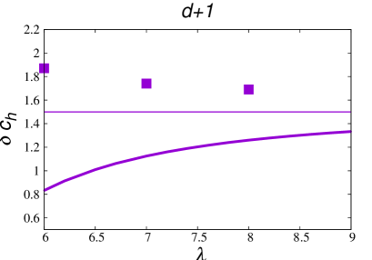
Figure 1: The jump in the specific heat of the Ising model on lattices at $d>4$ (squares, results of MC simulations [5]) and on an annealed scale-free network for $\lambda>5$, bold line equation (14). The thin line shows classical mean-field value $\delta c_{h}=3/2$. Although $\delta c_{h}(\lambda\to\infty)=\delta c_{h}(d\to\infty)=3/2$, the functions approach the mean-field limit from below and from above.

It is well known that Ising model on an annealed scale-free network is characterized by classical mean-field exponents at $\lambda>5$. As we have shown in this note, the mean-field behaviour does not concern the specific heat jump $\delta c_{h}$ at $\lambda>5$. The jump remains $\lambda$-dependent and reaches the mean-field value $\delta c_{h}=3/2$ only in the limit $\lambda\to\infty$. The function $\delta c_{h}(\lambda)$ is shown in figure 1. Similar effect has been observed for the Ising model on lattices at $d>4$. We show the results of MC simulations of $d=5,6,7$-dimensional lattices [5] in the figure too. Note, that although $\delta c_{h}(\lambda\to\infty)=\delta c_{h}(d\to\infty)=3/2$, the functions approach the mean-field limit from below and from above. Another essential difference between the behaviour of $\delta c_{h}$ in the Ising model on scale-free networks and on lattices is observed directly at the upper critical values of $\lambda$ and of $d$, respectively. While $\alpha=0$ in both cases, the overall behaviour of $c_{h}$ remains singular on lattices at $d=4$ (logarithmic singularity, $\hat{\alpha}=1/3$) whereas $\hat{\alpha}=-1$ for networks at $\lambda=5$ and hence $\delta c_{h}=0$. This last case provides an example where the logarithmic correction to scaling leads to smoothing of behaviour of the thermodynamic function at $T_{\textrm{c}}$.

Ukrainian 0

Стрибок теплоємностi моделi Iзiнга на безмасштабнiй мережi М. Красницька${}^{\textsf{\footnotesize{\mbox{?},\penalty 1000\mbox{?},\penalty 1000\mbox{?}}}}$, Б. Берш${}^{\textsf{\footnotesize{\mbox{?},\penalty 1000\mbox{?}}}}$, Ю. Головач${}^{\textsf{\footnotesize{\mbox{?},\penalty 1000\mbox{?}}}}$, Р. Кенна${}^{\textsf{\footnotesize{\mbox{?},\penalty 1000\mbox{?}}}}$

             
${}^{\textsf{\footnotesize 1}}$ Iнститут фiзики конденсованих систем НАН України,
вул. I. Свєнцiцького, 1, 79011 Львiв, Україна ${}^{\textsf{\footnotesize 2}}$ Iнститут Ж. Лямура, Унiверситет Лотарингiї, F-54506 Вандувр лє Нансi, Францiя ${}^{\textsf{\footnotesize 3}}$ Центр прикладної математики, Унiверситет Ковентрi, Ковентрi CV1 5FB, Англiя ${}^{\textsf{\footnotesize 4}}$ Коледж докторантiв статистичної фiзики складних систем, Ляйпцiг-Лотарингiя-Львiв-Ковентрi $({\mathbb{L}}^{4})$

References

- [1] Landau L.D., Lifshitz E.M., Statistical Physics, Course of Theoretical Physics, Vol. 5, 3rd Edn., Butterworth-Heinemann, Oxford, 1980.
- [2] Onsager L., Phys. Rev., 1944, 65, 117; doi:10.1103/PhysRev.65.117.
- [3] Guida R., Zinn-Justin J., J. Phys. A: Math. Gen., 1998, 31, 8103; doi:10.1088/0305-4470/31/40/006.
- [4] Kenna R., In: Order, Disorder and Criticality Advanced Problems of Phase Transition Theory, Vol. 3, Holovatch Yu. (Ed), World Scientific, Singapore, 2012, pp. 1–47.
- [5] Lundow P.H., Markström K., Nucl. Phys. B, 2015, 895, 305; doi:10.1016/j.nuclphysb.2015.04.013.
- [6] Albert R., Barabasi A.L., Rev. Mod. Phys., 2002, 74, 47; doi:10.1103/RevModPhys.74.47.
- [7] Holovatch Yu., von Ferber C., Olemskoi A., Holovatch T., Mryglod O., Olemskoi I., Palchykov V., J. Phys. Stud., 2006, 10, 247 (in Ukrainian).
- [8] Barrat A., Barthelemy M., Vespignani A., Dynamical Processes on Complex Networks, Cambridge University Press, Cambridge, 2008.
- [9] Newman M., Networks: An Introduction, Oxford University Press, Oxford, 2010.
- [10] Dorogovtsev S.N., Goltsev A.V., Rev. Mod. Phys., 2008, 80, 1275; doi:10.1103/RevModPhys.80.1275.
- [11] Lee S.H., Ha M., Jeong H., Noh J.D., Park H., Phys. Rev. E, 2009, 80, 051127; doi:10.1103/PhysRevE.80.051127.
- [12] Bianconi G., Phys. Rev. E, 2012, 85, 061113; doi:10.1103/PhysRevE.85.061113.
- [13] Dommers S., Giardina C., Giberti C., van der Hofstad R., Prioriello M.L., Preprint arXiv:1509.07327, 2015.
- [14] Stanley H.E., Introduction to Phase Transitions and Critical Phenomena, Oxford University Press, Oxford, New York, 1971.
-
[15]
Krasnytska M., Berche B., Holovatch Yu., Kenna R., Europhys. Lett., 2015, 111, 60009;
doi:10.1209/0295-5075/111/60009. - [16] Krasnytska M., Berche B., Holovatch Yu., Kenna R., J. Phys. A: Math. Theor. (in press); Preprint arXiv:1510.00534, 2015.
- [17] Leone M., Vázquez A., Vespignani A., Zecchina R., Eur. Phys. J. B, 2002, 28, 191; doi:10.1140/epjb/e2002-00220-0.
- [18] Dorogovtsev S., Goltsev A.V., Mendes J.F.F., Eur. Phys. J. B, 2004, 38, 177; doi:10.1140/epjb/e2004-00019-y.
-
[19]
Palchykov V., von Ferber C., Folk R., Holovatch Yu., Phys. Rev. E,
2009, 80, 011108;
doi:10.1103/PhysRevE.80.011108. -
[20]
Von Ferber C., Folk R., Holovatch Yu., Kenna R., Palchykov V., Phys. Rev. E, 2011, 83, 061114;
doi:10.1103/PhysRevE.83.061114.
Ukrainian \adddialect\l@ukrainian0 \l@ukrainian