The Physics of Water Masers observable with ALMA and SOFIA: Model Predictions for Evolved Stars

Abstract

We present the results of models that were designed to study all possible water maser transitions in the frequency range 0-1.91 THz, with particular emphasis on maser transitions that may be generated in evolved-star envelopes and observed with the ALMA and SOFIA telescopes. We used tens of thousands of radiative transfer models of both spin species of H₂O, spanning a considerable parameter space in number density, kinetic temperature and dust temperature. Results, in the form of maser optical depths, have been summarized in a master table, Table 6. Maser transitions identified in these models were grouped according to loci of inverted regions in the density/kinetic temperature plane, a property clearly related to the dominant mode of pumping. A more detailed study of the effect of dust temperature on maser optical depth enabled us to divide the maser transitions into three groups: those with both collisional and radiative pumping schemes (22,96,209,321,325,395,941 and 1486 GHz), a much larger set that are predominantly radiatively pumped, and another large group with a predominantly collisional pump. The effect of accelerative and decelerative velocity shifts of up to 5 km s^-1 was found to be generally modest, with the primary effect of reducing computed maser optical depths. More subtle asymmetric effects, dependent on line overlap, include maximum gains offset from zero shift by $>$1 km s^-1, but these effects were predominantly found under conditions of weak amplification. These models will allow astronomers to use multi-transition water maser observations to constrain physical conditions down to the size of individual masing clouds (size of a few astronomical units).

1 Introduction

Water masers from the $6_{16}-5_{23}$ transition of ortho-H₂O (o-H₂O) at 22.23508 GHz are abundant in star-forming regions, in the extended atmospheres of evolved stars and in some external galaxies (‘megamasers’). The original detection towards the Orion star-forming region (Cheung et al., 1969) was followed up by observations that included the red supergiant star VY CMa (Meeks et al., 1969). Modern surveys of star-forming and evolved star sources have been carried out, or are in progress. Probably the majority of work has concentrated on masers from star-forming regions, including both high-mass and low-mass sources.

Masers at 22 GHz, from any source type, are not the main focus of the present work, but 22 GHz is so far the only water maser frequency at which large-scale surveys have been carried out, giving us some idea of the Galactic distribution of sources. With the implicit assumption that the distribution of water masers at other frequencies broadly follows the 22-GHz distribution, we therefore initially consider 22-GHz surveys for all Galactic source types.

Selective surveys of water masers in high-mass young stellar objects (HMYSOs) (Urquhart et al., 2009, 2011) typically observe towards sources that satisfy certain infra-red colour criteria based, for example, on the Red MSX Source survey, or 4.5 $\mu$m emission detected by the GLIMPSE instrument aboard the Spitzer satellite (Yung et al., 2013). Unlike 6.7-GHz methanol masers that are believed to be associated only with the formation of high-mass stars (Xu et al., 2008), 22-GHz water masers are also associated with low-mass protostellar objects, and surveys of objects of this type include work by Furuya et al. (2001) and Furuya et al. (2003) (respective errata in Furuya et al. (2007b, a)) that showed that water masers are associated primarily with low-mass protostars of class 0 with some in class 1. No masers were found towards class 2 protostars or pre-stellar cores. An association with 100-AU-scale jets suggests that the water maser emission is coupled to shock waves, as in other source types. Hollenbach et al. (2013) and Kaufman & Neufeld (1996) showed that the conditions for shocks to excite water masers can occur in star-forming regions, notably (but not exclusively) due to the impact of protostellar jets, discussed further in Section 1.5. A caveat regarding such an interpretation is that the collimation and precession of jets is linked to variability of masers, so long-term monitoring of sources is preferable to observations at a single epoch. Other excitation schemes involve the boundaries of wide-angle outflows (Walker, 1984; Mac Low et al., 1994) and discs (Fiebig, 1997; Gallimore et al., 2003).

Detection of water masers towards only 5 of 99 observed low-mass protostars in Orion, selected on the basis on infra-red colours, suggests that water masers probably appear rarely in such objects (Kang et al., 2013). Water masers were found towards 9 per cent of the intermediate-mass objects observed by Bae et al. (2011), so the detection rate probably rises with protostellar mass. Water masers associated with HMYSOs are highly variable: a 20-yr study of 43 such objects by Felli et al. (2007) includes velocity-time-flux plots that may be used to compare short-duration features and more stable spectral components. Observations with the ATCA (Australia Telescope Compact Array) towards dust clumps emitting strongly at 1.2 mm (Breen & Ellingsen, 2011) revealed a much better correlation between 22-GHz masers in MYSOs and these clumps than is typically found for masers and infra-red colours. The 1.2-mm clumps associated with H₂O masers are of order 1 pc across.

Unbiased surveys of water masers naturally include sources of both protostellar and evolved-star types. Small-scale interferometric pathfinder surveys of the Galactic centre (Caswell et al., 2011) and other regions of the Southern Galactic plane (Caswell & Breen, 2010) with the ATCA show that variability on timescales of order 1 yr is common, that the spatial density of water masers exceeds that of methanol and OH, even in regions where the latter two species are known to be common, and that the positions of water maser sources are significantly more stable over time than their spectra. The spectral ranges of water maser sources were already known to exceed those typical of methanol and OH (Felli et al., 2007). In the sample observed by Caswell & Breen (2010), nine objects (28 per cent) exhibited extreme velocity spectral components, defined as separated from the systemic velocity by $>$30 km s^-1. These components, associated with outflows, are dominated by blue-shifted emission. The H₂O Southern Galactic Plane Survey (HOPS) (Walsh et al., 2011) surveyed 100 square degrees of the Southern Galactic plane with a broad-band spectrometer that included the 22-GHz water maser line amongst many other transitions down to an rms noise level of typically 1-2 Jy. The survey results suggest that 800-1500 22-GHz maser sources exist in the Milky Way down to this noise level. A scale-height of only 0.5$\degr$, similar to that for 6.7-GHz methanol masers, suggests that most HOPS detections are associated with high-mass star formation. This view has been confirmed by ATCA positional associations (Walsh et al., 2014) that identify, of the sources associated with otherwise known astrophysical objects, 69 per cent with star formation, 19 per cent with evolved stars and 12 per cent unknown.

It has long been known that individual 22-GHz water maser features are among the smallest and brightest known. Early global VLBI (Very Long Baseline Interferometry) experiments (Burke et al., 1972, 1973) determined that features as small as 300 microarcsec (4.5 AU) existed in the W49 star-forming region, with a brightness temperature of $T_{b}$ = 10¹⁵ K. A recent VLBI experiment with a space-based antenna (RadioAstron) found structure on a scale of only 10 microarcsec ($\sim$1 R_☉) in Cep A, with a brightness temperature of at least 1.5$\times$10¹⁴ K; a flare in Orion KL observed with HALCA (Highly Advanced Laboratory for Communications and Astronomy) (Omodaka et al., 1999) had a brightness temperature of 10¹⁷ K.

A single-dish survey of 401 evolved stars, mostly of Mira, OH/IR and semi-regular variable types, was used to calculate useful statistics for both the 22-GHz H₂O line, and the SiO 43-GHz masers from the vibrational states $v=1$ and $2$ (Kim et al., 2014). Results from such a single-phase snapshot of many sources are broadly consistent with those derived from long-term monitoring of a small number of sources over at least several stellar periods, an example of the latter type of observation being Lekht et al. (2005). The snapshot revealed that the 22-GHz masers are weaker (in photon luminosity, peak and frequency-integrated intensity) than the SiO masers at most stellar phases, but that the water masers become relatively more powerful as stars become more massive, and have greater mass-loss rates - that is as stellar properties move from the Miras to the OH/IR stars (Engels et al., 1986). More information about the effect of the circumstellar velocity field on the masers can be gleaned from the velocity extent and red/blue dominance in the spectra. In Mira variables, Kim et al. (2014) find a very similar spectral extent for SiO and H₂O 22 GHz masers (respectively 13.7 and 12.9 km s^-1). However, the H₂O emission becomes significantly broader in OH/IR stars (25.5 km s^-1 against 13.3). In both types, the SiO velocities are consistent with an average expansion velocity of $\leq$7 km s^-1 in the maser zone, as required by observational constraints (Reid & Menten, 2007). Individual 22-GHz H₂O maser sources show a wide range of values for the expansion velocity, with spectral extents exceeding 40 km s^-1 for supergiants and some OH/IR stars, whilst Miras have values between 4 and $\sim$40 km s^-1. For example, VLBI observations of RT Vir (Imai et al., 2003) found an approximate velocity of expansion of 8 km s^-1 in the water maser zone. Infra-Red Astronomy Satellite (IRAS) colour-colour diagrams in Kim et al. (2014) indicate that H₂O masers form at an earlier evolutionary stage than SiO masers, but the H₂O masers may also persist into the PPN (proto-planetary nebula) stage, probably in a new form dominated by asymmetric outflow. Development of water (and SiO) maser emission in the transition from AGB (Asymptotic Giant Branch) to post-AGB stars is surveyed in more detail in Yoon et al. (2014).

The influence of pulsation shocks on 22-GHz H₂O masers is not clear. Model predictions (for example Ireland et al. 2008, Ireland et al. 2011) are of weakening shocks with increasing radius. Elitzur et al. (1992) modelled the different appearance of maser beaming from quiescently expanding clouds or shocked slabs, and Richards & et al. (2010) showed that the symptoms of shocks are only observed in a minority of clouds, mostly in the thinner-shelled CSEs in the study. This is consistent with the predictions of Ireland et al. (2008). However, in this context, one would expect to see evidence for shocks close to the inner rim of the water maser shell, but Imai et al. (2003) observed a shock-accelerated feature further out in the shell around RT Vir, and VY CMa also shows evidence that suggests shocks far from the star (Section 1.2). It is clear that shocks alone cannot explain water maser variability, since monitoring shows that features throughout the entire 22-GHz shells (perhaps 15/150 AU thick around AGB/RSG stars) vary in concert within weeks to years - much faster than even a highly supersonic shock.

The 22-GHz transition remains by far the most widely studied, but maser action has been confirmed in several more lines at higher frequencies. Twelve (possibly thirteen) additional maser transitions were tabulated in Humphreys (2007), and a similar list of eleven maser transitions appears in Chapter 2 of Gray (2012). A newer search for detected masing lines in the literature shows that at least 18 transitions have now been identified as masers in addition to 22 GHz (see entries with Y in the final column of Table 1 and the text of Section 2.1). More maser transitions will almost certainly be identified in future, and it is worth noting that several high frequency lines that were detected with Herschel at low spectral resolution (Matsuura et al., 2014) are predicted to be masers in this work, and are listed in Table 6. Most of the known high-frequency masers in Table 1, like 22-GHz, have been detected towards both star-forming regions and evolved stars. However, a sub-set of maser transitions within the first excited state of the vibrational bending mode ($v_{2}=1$), and two $v_{2}=2$ maser transitions, have been detected exclusively towards evolved stars (see final column of Table 1 and footnotes).

Almost all of the high-frequency water masers have rest frequencies above 100 GHz, making them difficult to observe from low-altitude sites. They have been much less useful scientifically than the 22-GHz transition because, prior to the advent of ALMA, there were few interferometric observations of any of the high-frequency lines, and none to compare with the milli-arcsecond resolution typically achieved with continental VLBI at 22 GHz. ALMA offers the exciting possibility of extending routine interferometric observations with angular resolution of typically tens of milli-arcseconds to most of the known mm-wave and sub-mm water maser transitions. SOFIA is a single-dish instrument, but provides a new window that may allow us to detect new water maser transitions with frequences greater than 1 THz.

1.1 Water masers in AGB and post-AGB stars

Work on high-frequency water masers prior to 2007, including most of the initial detections, has been reviewed by Humphreys (2007). An exception is the interferometric work carried out with the Submillimeter Array (SMA) on the 658-GHz transition (Hunter et al., 2007), a transition in the $v_{2}=1$ bending mode of o-H₂O, where the lower energy level of the transition lies at 2297 K above the ground state. In a sample of four Mira variables, the spectral width of the 658-GHz line was found to be similar to that of the SiO $v=1,J=5-4$ line at 215 GHz. This similarity, and comparable energies above ground for the lower maser levels, suggest that these o-H₂O and SiO transitions originate from a similar region: the SiO zone that lies much closer to the star ($<$ 5 stellar radii) than is typical for 22-GHz water masers. The 22-GHz maser shell, resolved by interferometry, typically extends from about 5 to 20 stellar radii, over which distance the expansion velocity approximately doubles, exceeding the escape velocity in the process (for example, Richards et al. 2012).

The Mira R Leo and the semi-regular variable W Hya were observed in eight sub-millimetre water transitions with APEX (Atacama Pathfinder EXperiment) (Menten et al., 2008). The very high excitation line at 354.8 GHz (17_4,13-16_7,10) was not detected towards either source, despite predictions of inversion by Neufeld & Melnick (1991) and Yates et al. (1997) (respectively NM91 and YFG97). However, both sources exhibited strong masers at 437.3 GHz, and weaker emission at 443.0 GHz, that are not predicted by NM91. Photon luminosities of the detected lines, and the velocity extents of the spectra, were consistent with the detected lines arising from approximately the same region of the outflowing atmosphere. In R Leo, near contemporary 22-GHz observations showed that this line was anomalously weak, whilst the 437-GHz maser was much stronger than the others. These observations also resulted in the first detection of a maser at 474.7 GHz - a line predicted by NM91, but only at the higher temperature of 1000 K, and by YFG97. Herschel HIFI (Heterodyne Instrument for the Far Infrared) observations (Justtanont et al., 2012) detected 658-GHz masers towards several AGB stars with new maser detections at 620.7 GHz towards IRC+10011, W Hya and IK Tau and possible masers at 970.3 GHz towards the latter two stars.

A type of post-AGB star, known as a water-fountain source, has evolved to a state in which a fast, highly asymmetric post-AGB outflow is interacting with the older spherically symmetric shell from the AGB phase. Water masers form in the interaction zone of the fast and slow outflows. Tafoya et al. (2014) studied seven water fountain sources with APEX, detecting 321-GHz H₂O masers towards three of them, but detecting no emission at 325 GHz. The breadth of the 321-GHz spectrum ($>$100 km s^-1) links these masers to the fast wind, rather than the AGB material that has an expansion velocity of only $\sim$20 km s^-1. In two of the sources, the authors co-locate the 321-GHz and 22-GHz masers, but invoke a more complicated model for the third source, where the spectral widths of the maser lines are substantially different.

1.2 Water masers in red supergiants

Although the known water-masing red supergiants (RSGs) are at ditances $>$800 pc, they have bright 22-GHz masers and searches for higher transitions have been fruitful, especially in VY CMa, for example Menten & Melnick (1989), Menten et al. (1990), and see Table 1. High frequency lines have also been detected from other RSGs, for example 321- and 325-GHz emission (Yates et al., 1995), 658-GHz (Menten & Young, 1995) from NML Cyg and VX Sgr, plus 183-GHz emission also from S Per and $\mu$ Cep (Gonzalez-Alfonso et al., 1998).

VY CMa has the brightest water masers and the largest CSE, and has been studied in the most detail. Specific properties of VY CMa are summarized in Meeks et al. (1969). This star was one of the four bright sources that were the subject of the first interferometric observations of 22-GHz water masers (Burke et al., 1970), and it is also a source of several mm-wave and sub-mm water masers. VY CMa was among the stars observed by Hunter et al. (2007), who showed that its 658-GHz emitting region is unresolved at scales of $\sim$1$\aas@@fstack{\prime\prime}$

VY CMa was also a target of the multi-frequency APEX observations by Menten et al. (2008). Detections were achieved in seven of the nine transitions observed, and all had photon luminosities between 6 $\times$ 10⁴⁴ and 5 $\times$ 10⁴⁵ s^-1, some three orders of magnitude more powerful than typical values for AGB stars. The photon luminosity of the 22-GHz maser in VY CMa is similar to the level of its sub-mm lines. A distinct difference between VY CMa and AGB stars is in the width and shape of its maser spectral profiles: each profile is remarkably individual in VY CMa, suggesting different regions of origin, whilst the profiles from AGB stars have similar widths for a given object. The VY CMa spectra are also typically very broad ($>$50 km s^-1) compared to a few km s^-1 in AGB stars. The 437-GHz line, not predicted by NM91 or YFG97, was also detected towards VY CMa.

SMA observations of VY CMa (Kamiński et al., 2013) included six water transitions in the frequency range 293-337 GHz. The interferometer did not resolve the emission in any of these transitions (synthesized beam of approximately 0$\aas@@fstack{\prime\prime}$9). The expected ground vibrational state masers at 321 and 325 GHz were accompanied by a possible weak maser in the ($0,1,0$) state at 293.7 GHz.

By far the most detailed information about a subset of sub-mm water maser lines (at 321, 325 and 658 GHz) comes from ALMA observations (Richards et al., 2014). For the first time, the continuum emission and masers were, simultaneously, well resolved, establishing the almost certain site of the star to coincide with the centre of the water maser expansion, some 0$\aas@@fstack{\prime\prime}$4 to the North-West of the brightest continuum region. With spatial resolution as good as 60 milliarcsec at 658 GHz, the spatial relationship of maser features at the three sub-mm frequencies, and at 22 GHz, could be established. While the maser features share a common sky-plane area up to $\sim$1 arcsec ($\sim$850 AU) in diameter, they rather avoid each other at smaller scales, consistent with significantly different pumping regimes. Linear distributions of masers with a velocity gradient are common. Although the 658-GHz masers are mainly concentrated in the central 0$\aas@@fstack{\prime\prime}$1, as expected for a transition with its lower level so far above ground, some 658-GHz masers are found much further from the star, and this behaviour is unexplained. It was suggested that the farthest-out 658-GHz masers could be excited by shocks in the stellar wind, for example from the collision of fast-flowing material with more slowly moving dense clumps.

The 620.7-GHz transition was detected as a maser for the first time towards VY CMa by Harwit et al. (2010) with the HIFI instrument aboard HERSCHEL. Their experiment was polarization sensitive, and found negligible polarization near the peak of the line, but rising values to $\sim$6 per cent in the line wings, in a manner that is consistent with the theory by Goldreich & Kylafis (1981). The same instrument also detected the 970.3-GHz transition as a maser (De Beck et al., 2011). SPIRE (Spectral and Photometric Imaging Receiver) and PACS (Photoconductor Array Camera and Spectrometer) observations of VY CMa detected a number of emission lines of water that may be masers (Matsuura et al., 2014) at 1158.3,1172.5,1278.3,1296.4,1308.0,1322.1,1435.0 and 1440.8 GHz. These transitions are all predicted to be strongly inverted in our Table 6. The limited resolution of the HERSCHEL observations makes it difficult to tell whether there are masers in these transitions. Numerical fits that accompany the observations agree with our predictions of inversion in 7 out of 9 cases, the exceptions being 1435.0 and 1542.0 GHz. Similar HIFI observations of VY CMa by Alcolea (2013) find emission in 7 additional transitions at 968.0,970.3,1000.9, 1153.1,1205.8,1718.7 and 1753.9 GHz that are in our table of maser predictions, Table 6. The 968-GHz transition is particularly identified as a maser, though the velocity resolution of about 1 km s^-1 is arguably not good enough to confirm this. One additional transition at 1194.8 GHz is claimed by Alcolea (2013) as a possible maser, but is not predicted to be so in this work.

1.3 Water masers in star-forming regions

As for evolved stars, most work on water masers other than 22 GHz, prior to 2007, is summarised in Humphreys (2007). The range of transitions found as masers in star-forming regions was long thought to be restricted to the vibrational ground state, but is now known to include masers from the bending mode, $v_{2}=1$. It is also notable that 183.3-GHz masers cover an extended region in Orion IRc2 (as covered by a mosaic of IRAM 30-m observations), and these appear to be generated under conditions that are too cold and rarefied to be considered in the usual shock-style pumping schemes (Cernicharo et al., 1994). A similar conclusion was reached for 325.2-GHz masers from the same source (Cernicharo et al., 1999). The 183-GHz line is one of very few masers to be observed towards low-mass protostellar objects: for example, 3 emission spots were detected towards Serpens SMM1, a class 0 low-mass protostar envelope with a mass of only 2.7 M_☉ (van Kempen et al., 2009). This detection supports the view that 183-GHz masers can be pumped in cooler, more rarified, conditions than those at 22 GHz.

The first imaging observations of the 321-GHz, 10_2,9-9_3,6 transition of o-H₂O with the SMA (Patel et al., 2007) revealed that, in Ceph A, the distribution of these masers lies along the jet of a disc-outflow system, while 22-GHz masers in this source are associated with the disc. SMA observations were also made in the 183-GHz line of p-H₂O towards Serpens SMM1. As for the 321-GHz maser in Cepheus A, the 183-GHz emission appears associated with a protostellar jet, and is spatially distinct from 22-GHz features.

The advent of ALMA observations has led to significantly more detailed information in some transitions, particularly towards the relatively close high-mass star-forming region Orion KL. Hirota et al. (2012) (and see also the erratum in Hirota et al. 2014) detected the $v_{2}=1$ line at 232.7-GHz towards Orion KL; previously this maser transition was known only in evolved star envelopes. The 232.7-GHz emission was clearly associated with Source I, but the maser distribution was not resolved. The 232.7-GHz spectrum was more similar to that of 22-GHz water masers than to that of SiO masers. 325-GHz masers in Source I were imaged with the SMA by Niederhofer et al. (2012). These masers trace a collimated outflow, with rotation, and probably sample similar pumping conditions to 22-GHz masers. Emission at 321 GHz towards Orion Source I may be of maser origin and appears to sample similar conditions to 43-GHz SiO masers (Hirota et al., 2014).

The HERSCHEL spacecraft has much poorer spatial resolution than ALMA, but it has the advantage of observing free from atmospheric absorption that becomes increasingly problematic at frequencies $>$500 GHz. The 620.7-GHz (5_3,2-4_4,1) transition was detected as a maser by Neufeld et al. (2013) towards Orion KL, Orion S and W49, with clear variability over 2 yr in the last source. The 620.7-GHz line appears to be pumped under physical conditions that are a subset of those that pump 22-GHz masers. The same HERSCHEL instrument (HIFI) was used by Jones et al. (2014) to study polarization and variability properties of the 620.7-GHz masers in Orion KL. No significant polarization was found ($<$2 per cent), but whilst some spectral features at 22-GHz show strong polarization (up to 75 per cent), the one closest in velocity to the 620.7-GHz line exhibits much weaker polarization of order 10 per cent.

1.4 Extragalactic water masers

Extragalactic water megamasers are a well-known phenomenon, and have been employed, via their arrangement in discs with Keplerian rotation, as tools to measure geometrical distances to NGC4258 and other galaxies (Braatz et al. 2010 and references therein). High-frequency water masers are also observed towards some megamaser sources, based on active galactic nucleus (AGN) excitation. 183 and 439-GHz lines were detected towards NGC3079 by Humphreys et al. (2005). Emission at 183 GHz without accompanying masers at 22-GHz has been observed towards Arp 220 (Cernicharo et al., 2006). More recent ALMA observations detected 321-GHz masers in the Circinus galaxy (Hagiwara et al., 2013), but these extragalactic sources will not be considered in detail here.

1.5 Water maser theory and modelling

The pumping mechanism of the 22-GHz water maser has long been understood in general terms, with a model going back as far as the work of de Jong (1973). Put simply, efficient radiative coupling of the ‘backbone’ levels (those that have the smallest allowed value of $K_{a}$ for a given value of $J$) preserves near-Boltzmann populations in these levels, while significant departures from Boltzmann predictions appear in the populations of non-backbone levels. The upper level of the maser, $J_{K_{a},K_{c}}=6_{1,6}$, is a backbone level, but the lower level, $5_{2,3}$, can be drained efficiently into a lower backbone level, $4_{1,4}$, by collisions and spontaneous emission. A similar explanation can immediately be applied to other maser transitions where the upper level is a member of the backbone, namely 183, 325 and 380 GHz.

Detailed explanations of the 22-GHz maser pump in terms of a dissociative J-type shock were introduced by Elitzur et al. (1989), where masers form in the cooling post-shock gas following the chemical re-formation of water. Extension to non-dissociative MHD shocks was carried out by Kaufman & Neufeld (1996), and these models can produce water at a typically higher temperature in the maser zone than J-shocks. This appears to make C-type shocks the more likely site of masers from transitions with lower levels $\ga$1000 K. More recent work (Hollenbach et al., 2013) has revisited J-shocks as the maser formation zone, establishing likely boundaries in density and shock velocity for the formation of saturating 22-GHz masers in both C-type and J-type shocks. It is important to note that the aspect ratios of masers formed in shocks generally, and J-shocks in particular, are large (Hollenbach et al., 2013), that is they are typically 30-100 times more extended parallel to the shock than perpendicular to it, and are therefore strongly beamed parallel to the shock front.

Models involving many levels and transitions of water, including most of the known water masers, have been used to test understanding of the basic pumping scheme, and to make predictions of additional masers. The best known works of this type are probably NM91 and YFG97. The former used escape probability methods, whilst the latter used accelerated lambda iteration (ALI) to compute molecular energy level populations, as does the present work. However, both NM91 and YFG97 used molecular data that has since been superceded, and neither allowed for far-infrared line overlap. NM91 showed that the collision plus spontaneous emission pumping scheme, as usually applied to 22-GHz masers, actually applies also to the great majority of the then known higher frequency water masers. YFG97 showed that some transitions, for example those at 437, 439 and 471 GHz are best pumped by a strong infra-red continuum radiation field, for example from dust local to the maser zone.

Studies of extended (15”$\times$15”) 183-GHz maser emission towards Sgr B2(M) (Cernicharo et al., 2006) included both LVG (Large Velocity Gradient) and more exact radiative transfer models to obtain the physical conditions. To explain this extended emission requires a very different regime from that considered by most models, including NM91 and YFG97. The dominant pumping process for the 183-GHz masers in this source is radiative, driven by FIR photons, and covers a density and temperature regime that is only at $T_{K}\sim 30$ K and $n_{H_{2}}\sim 10^{5}-10^{6}$ cm^-3. The LVG models demonstrate the switch to the conventional collision-based pumping scheme at higher temperatures (400-500 K). The 183-GHz maser in O-rich evolved star envelopes was modelled by González-Alfonso & Cernicharo (1999), using LVG and exact methods. A significant radiative component to the pumping mechanism was found for stars of higher mass-loss rates, proceeding through radiative excitation of the first excited state of the vibrational bending mode.

A model of the water masers in a pulsating AGB star (Humphreys et al., 2001) was one of the first to try and establish the spatial relationship of the principal mm-wave and sub-mm masers, and the possibility of their co-existence with each other and with 22-GHz masers. This model represented the maser clumps as LVG blocks with physical conditions drawn from a pulsating atmosphere model of a Mira variable (Bowen, 1988). The pulsating atmosphere provides radial shock-waves, attenuating with increasing radius. By $\sim$5 R_∗, maser emission from many 22-GHz clouds appears consistent with a smoother, radial outflow, although wind clumping and changes in mass loss rate may lead to shocks at larger radii. Humphreys et al. (2001) classified the water masers into three groups: the first, with 321 GHz as the prototype, lie close to the star (radial extent 2-5 R_∗), sampling similar conditions to SiO masers, and emit tangentially with emission dominated by a few bright spots. Group 2, exmplified by 22- and 325-GHz masers have a moderate extent, with most emission in the range 2-10 R_∗, peaking in the zone where the motion of the gas is changing from radial pulsation towards a steady outflow, but we note that 22-GHz masers are found closer to the star in the model than in observations. A third group, with 183 GHz as the prototype, have an even larger extent (2-20 R_∗) with mostly radial emission provided by a very large number of comparatively weak spots. Humphreys et al. (2001) did not include any vibrationally excited states of water, and so were unable to make predictions about the 658-GHz line. An early attempt to model the $(0,1,0)$ vibrational state (Deguchi, 1977) did not find this transition to be inverted, but recent work (Nesterenok, 2015) reproduces the maser, using the same molecular data as the present work.

Recent ALI modelling of the 22-GHz maser with up-to-date molecular data (Nesterenok, 2013) reinforces the usual view that a substantial radiation field in the far- and mid-infra-red is harmful to the 22-GHz inversion.

Polarization in H₂O maser transitions other than 22 GHz has been considered by Pérez-Sánchez & Vlemmings (2013) in the regime where the magnetic field defines a good quantization axis, but where the Zeeman rate is much smaller than the inhomogeneous line width. However, we do not model the Zeeman structure of H₂O in the present work.

1.6 Origins of clumping

In circumstellar envelopes, 22-GHz H₂O masers are observed to arise from clumps of gas with a size that correlates with the stellar radius (Richards et al., 2012). In the smaller types (for example Miras and semi-regular variables) the cloud size is apparantly restricted enough to make most masers unsaturated. The H₂O maser zone encompasses the critical range of radii where the radial velocity passes through the gravitational escape velocity, and periodic pulsations develop into a smooth wind. In fact, we observe this wind as a two-phase medium, with warm, dense clumps, suitable for pumping water masers, enclosed within a more rarefied phase that supports OH main-line maser emission (Richards et al., 1999). The density contrast between the phases has been calculated to be of order $10-100$ (Richards et al., 2011), with the filling factor of the dense clumps likely to be no more than 0.01.

Consideration of typical main-line pumping conditions for OH masers (for example Field et al. 1994) strongly suggests that the more rarefied phase is also cooler than the H₂O clouds. If this is so, the denser phase is over-pressured with respect to the more rarefied phase, and must be unstable unless otherwise constrained, for example by locally strong magnetic fields. If the clumps are indeed pressure unstable, they should disperse over the order of a dynamical time of $t\sim L/c_{s}$, where $L$ is the cloud scale and $c_{s}$, the sound speed in the clump. Expanding this formula, the expected dispersal time is

$$\tau=1.98[\bar{\mu}/(\gamma_{7/2}T_{1000})]^{1/2}L_{AU}\;\;\mathrm{yr},$$ (1)

where $\bar{\mu}$ is the mean molecular mass in H₂ units, $\gamma_{7/2}$ is the ratio of specific heat capacities relative to that for a rigid diatomic molecule, and $T_{1000}$ is the temperature in units of 1000 K. It appears that an additional constraint mechanism is required, since individual maser clumps survive for decades (comparable to the crossing time of the 22-GHz maser shell, Richards et al. 2012) even though their maser brightnesses may fluctuate on timescales of 5 yr or less.

Theoretically, we can understand a bifurcation of the medium arising in the SiO zone via thermal and magneto-thermal instabilities (Cuntz & Muchmore, 1989, 1994; Neufeld & Kaufman, 1993; Gray et al., 1998). Regions of gas that are well cooled by radiation from rovibrational transitions of CO and H₂O go on to become dense clouds that support SiO and H₂O maser emission, and probably also have a greater abundance of these molecules than their surroundings. The possible collision of the rarefied and dense components of the gas at larger radii (the water-maser zone) may cause additional shocks in some stars, plausibly resulting in the observed linear features in VY CMa (Richards et al., 2014). An additional source of shock heating is certainly attractive, since the radial stellar pulsation shocks become much attenuated as they progress through the water maser zone (Bowen, 1988; Humphreys et al., 2001). Both shock mechanisms however lead to variability of the water masers on typical timescales of months to years.

Although an explanation in terms of instabilities, with an associated physical scale corresponding to an optimum growth rate, may at first appear to be at odds with the observed scaling with star size (Richards et al., 2012), the observation and clumping theory may still be compatible. Recent work (Gray et al. in preparation) on instabilities in a spherical geometry generates perturbations in terms of spherical harmonics that have a natural radial scaling as a multiple of the stellar radius.

2 Observational Possibilities for Water Masers

There is a long history observing the 22-GHz maser line with many instruments, including VLBI; other telescopes have been mentioned in Section 1. At higher frequencies, single dishes and arrays such as IRAM and SMA have provided first detections of a number of other bright water masers but in most cases are unable to resolve them alone. VLBI instruments such as, for example, the KVN (Korean VLBI Network) and GMVA (Global mm-VLBI) could be employed to study the 67- and 96-GHz lines if new receivers become available. However, water masers will be an ideal target for ALMA, which can already observe high-frequency cicumstellar H₂O masers interferometrically. There are no current instruments covering most of the spectral regions between 0.1 and 1.2 THz that are not covered by ALMA bands. One maser transition that falls outside the ALMA bands is at 380 GHz, detected by the Kuiper Airborne Observatory (Phillips et al., 1980). At frequencies above the upper limit of ALMA, the emphasis is more on detection of hitherto unobservable H₂O maser lines, rather than on high-resolution imaging, and SOFIA has two useful observing bands at frequencies above 1 THz. The availability of a new generation of instruments, but particularly ALMA and SOFIA, make it timely to produce fresh models of the inversions in water transitions at frequencies from 0 to 1.91 THz. The capabilities of ALMA and SOFIA, with particular attention to maser observations, are considered below.

2.1 ALMA Observations

ALMA will eventually observe in all the atmospheric windows between 31.3 and 950 GHz, specifically: 31-45, or perhaps 35-52, GHz (Band 1), 65-90 GHz (Band 2), 84-116 GHz (Band 3), 125-163 GHz (Band 4), 163-211 GHz (Band 5), 211-275 GHz (Band 6), 275-373 GHz (Band 7), 385-500 GHz (Band 8), 602-720 GHz (Band 9) and 787-950 GHz (Band 10). Bands 1, 2 and 5 are not yet (2016) available. Taking 30-80 mas resolution as an example, and with at least 36 12-m antennas, we achieve, after 5 minutes observing on-source, a 4-sigma brightness temperature sensitivity of around 5$\times$10⁴ K or better in all bands, except for a few masers lying in the worst regions for atmospheric transmission where 10-15 minutes are required. This assumes a velocity resolution of  0.1 km s^-1 in a maximum velocity span of  150 km s^-1 per spectral window (spw). At $\lambda=3$ mm (Band 3) this velocity resolution requires the finest normally-available frequency resolution of 32.278 kHz in dual polarization (taking on-line Hanning smoothing into account). The velocity resolution at longer wavelengths is broader in proportion to the wavelength, or narrower resolution is similarly possible at shorter wavelengths, down to 0.01 km s^-1 in Band 10 (0.3 mm wavelength), a spectral resolving power of 3$\times$10⁷. The correlator was designed to reach 3.8 kHz resolution in single polarization in a limited total bandwidth, but spectral resolution may in practice be limited by other factors.

ALMA can observe multiple spw in different configurations in four 2-GHz basebands, subject to placement rules, allowing several spectral lines to be observed simultaneously (within a band-dependent maximum span) and for the stellar continuum to be detected, facilitating alignment of observations taken at different times.

In Table 1, we list the known water maser lines from both water spin species, locating them within an ALMA band where possible. We exclude transitions with frequencies below 65 GHz that may fall into the currently unavailable band 1 and the 380.2-GHz line between bands 7 and 8, and detected from the KAO (Phillips et al., 1980). Also included in Table 1 are a number of predicted maser lines from NM91 and YFG97 that should be reasonably clear of atmospheric extinction. We note that the transitions at 645.77,645.91,863.84 and 863.86 GHz are not predicted to be strong masers in the present work.

Table 1: Known and predicted H₂O masers observable by ALMA

$\nu$	Transition	Spin	A-value	Band	Known
GHz	$J^{\prime}_{K^{\prime}_{a},K^{\prime}_{c}}-J_{K_{a},K_{c}}$	o/p	Hz
67.804	$(4_{1,4}-3_{2,1})^{*}$	o	1.950(-7)	2	N
96.261	$(4_{4,0}-5_{3,3})^{*}$	p	4.76(-7)	3	Y(M89)
183.31	$3_{1,3}-2_{2,0}$	p	3.65(-6)	5	Y(C90)
232.69	$(5_{5,0}-6_{4,3})^{*}$	o	4.76(-6)	6	Y(M89)
268.15	$(6_{5,2}-7_{4,3})^{**}$	o	1.53(-5)	6	Y(T10)
293.66	$(6_{6,1}-7_{5,2})^{*}$	o	7.22(-6)	7	Y(M06)
297.44	$(6_{6,0}-7_{5,3})^{*}$	p	7.51(-6)	7	Ya(K13)
321.23	$10_{2,9}-9_{3,6}$	o	6.16(-6)	7	Y(M90a)
325.15	$5_{1,5}-4_{2,2}$	p	1.17(-5)	7	Y(M90b)
331.12	$(3_{2,1}-4_{1,4})^{**}$	o	3.38(-5)	7	Ya(K13)
336.23	$(5_{2,3}-6_{1,6})^{*}$	o	1.08(-5)	7	Y(F93)
354.81	$17_{4,13}-16_{7,10}$	o	9.21(-6)	7	Y(F93)
390.13	$10_{3,7}-11_{2,10}$	p	8.51(-6)	8	N
437.34	$7_{5,3}-6_{6,0}$	p	2.15(-5)	8	Y(M93)
439.15	$6_{4,3}-5_{5,0}$	o	2.82(-5)	8	Y(M93)
443.02	$7_{5,2}-6_{6,1}$	o	2.23(-5)	8	Y(M08)
470.89	$6_{4,2}-5_{5,1}$	p	3.48(-5)	8	Y(M93)
474.69	$5_{3,3}-4_{4,0}$	p	4.82(-5)	8	Y(M08)
488.49	$6_{2,4}-7_{1,7}$	p	1.38(-5)	8	N
620.70	$5_{3,2}-4_{4,1}$	o	1.11(-4)	9	Y(H10)
645.77	$9_{7,3}-8_{8,0}$	p	4.62(-5)	9	N
645.91	$9_{7,2}-8_{8,1}$	o	4.62(-5)	9	N
658.01	$(1_{1,0}-1_{0,1})^{*}$	o	5.57(-3)	9	Y(M95)
863.84	$10_{8,3}-9_{9,0}$	o	9.46(-5)	10	N
863.86	$10_{8,2}-9_{9,1}$	p	9.46(-5)	10	N
906.21	$9_{2,8}-8_{3,5}$	p	2.22(-4)	10	N

Note that transitions surrounded by $()^{*}$, $()^{**}$ are respectively in the $v_{2}=1,2$ or $(0,1,0),(0,2,0)$ excited states (the first and second excited states of the bending mode). All other transitions are in the vibrational ground state.
Transitions in the $(0,2,0)$ vibrational state were observed by Tenenbaum et al. (2010) (T10).
Superscript ^∗∗ indicates a $(0,2,0)$ line present in the Kamiński et al. (2013) (K13). Supescript ’a’ indicates a line not identified as a water line but present in the spectral survey by Kaminski et al. (2013)(K13). Codes for other first detections are given in the final column of the table as follows:
M89 - Menten & Melnick (1989);C90 - Cernicharo et al. (1990)
M06 - Menten et al. (2006);M90a - Menten et al. (1990)
M90b - Menten et al. (1990);F93 - Feldman et al. (1993)
M93 - Melnick et al. (1993);M08 - Menten et al. (2008)
H10 - Harwit et al. (2010);M95 - Menten & Young (1995)

2.2 SOFIA Observations

SOFIA is an airborne infra-red telescope. Details of the project, and the observers’ handbook, may be obtained from the observatory web page. At typical operational altitudes, the telescope is above 99 per cent of the atmospheric water vapour, and atmospheric transmission is typically above 80 per cent. However, there are are still several frequency bands where the atmospheric opacity is severely limiting. The 2.7-m main mirror (effective area corresponds to a 2.5-m instrument) gives a 16″ beam at a wavelength of 160 $\mu$m.

For H₂O maser observations, the most useful instrument on board SOFIA is the heterodyne spectrometer, GREAT (German REceiver for Astronomy at Terahertz frequencies). This has, in principle, five spectral windows in the frequency range 1.2-5 THz. However, as of Cycle 3, only the lowest frequency pair, L1 and L2, were suitable for maser observations. Owing to atmospheric opacity, the L1 window is split into two sub-bands from 1.262 to 1.396 and from 1.432 to 1.523 THz. The L2 window is 1.800-1.910 THz. GREAT feeds a backend system that features two possible Fourier transform spectrometers. The higher and lower resolution instruments offer respective frequency resolutions of 44 and 212 kHz, which are adequate to resolve maser and thermal lines.

Unlike ALMA, SOFIA does not have the spatial resolution necessary to resolve water masers in circumstellar envelopes and star-forming regions. However, it does have the capacity to make new detections, and we list below likely target lines in Table 2. The transitions have been selected from NM91 and YFG97, and are therefore all in the vibrational ground state.

Table 2: Predicted H₂O maser lines observable by SOFIA

$\nu$	Transition	Spin	A-value	Band
GHz	$J^{\prime}_{K^{\prime}_{a},K^{\prime}_{c}}-J_{K_{a},K_{c}}$	o/p	Hz
1269.3	$13_{3,11}-12_{4,8}$	p	5.57(-4)	L1lo
1278.5	$7_{4,3}-5_{5,2}$	o	1.55(-3)	L1lo
1295.6	$8_{2,7}-7_{3,4}$	o	1.07(-3)	L1lo
1308.5	$8_{4,5}-9_{1,8}$	o	2.60(-4)	L1lo
1321.8	$6_{2,5}-5_{3,2}$	o	2.33(-3)	L1lo
1345.0	$7_{4,4}-8_{1,7}$	p	2.55(-4)	L1lo
1435.8	$9_{4,6}-10_{1,9}$	p	3.33(-4)	L1hi
1440.3	$7_{2,6}-6_{3,3}$	p	2.30(-3)	L1hi
1885.0	$8_{4,5}-7_{5,2}$	o	7.40(-3)	L2
1901.9	$12_{3,10}-11_{4,7}$	o	2.75(-3)	L2

3 The Model

There are perhaps two viewpoints that one may take when constructing a computational model of maser action, or for that matter, of any radiation transfer problem. The first is to select a particular source, and attempt to model its geometry, dynamics and other physical properties as accurately as possible, while accepting that the resulting model may have a very limited predictive power when applied to other sources. The second viewpoint, and this is the one adopted in the present work, is to run a very large number of fairly simple models, sampling a large parameter space in temperature, density and velocity fields, while accepting that none of these models apply very well to any individual source.

The computational results discussed below were produced by the code mmolg, an ALI radiation transfer code with a slab geometry. This code is indeed a direct development of that used by YFG97, and is based on an original code by Scharmer & Carlsson (1985). The major improvement of mmolg over the code used by YFG97 is the incorporation of local (from thermal and microturbulent widths) and non-local (from bulk velocity gradients) line overlap. The general overlap theory for mmolg is based on Stift (1992), and is also written down in Gray (2012). The line overlap operates within each water spin-species, but does not couple them radiatively, so that o-H₂O and p-H₂O were modelled independently. mmolg also benefits from an improved dust model, and more modern molecular data (see below). An increased number of levels and transitions makes line overlap more probable: in a typical example from p-H₂O, a total of 7341 radiative transitions were compressed into 6503 overlapping groups or blends, with a maximum overlap order (largest number of lines in a single group) of 10. The lowest frequency transition affected by overlap was 1428 GHz, so overlap does not affect the propagation of any masers visible to ALMA, but may, under rather extreme conditions, influence some target transitions for SOFIA.

The slab geometry used in the current work is probably not ideal, but is not unreasonable given the linear shock-based observational features that are frequently identified in the water-maser zones of evolved stars. Two cloud scales were used to represent, respectively, maser features in AGB stars and supergiants. For the former model, the total thickness of the water-containing slab was 4.5$\times$10¹³ cm (approximately 3 AU), whilst in the latter case 2.25$\times$10¹⁴ cm (15 AU) was used. In both cases, this water-containing slab was divided into 80 logarithmically-spaced layers, except for certain test models where a different number of layers was used to check invariance. In addition to the water-bearing slab discussed above, a further 5 layers were added to the side of the slab further from the observer. These layers have an exponentially decreasing abundance of water, and an exponentially increasing continuum opacity for the purpose of enforcing an optically thick boundary condition on the slab.

Silicate dust was modelled by means of the optical efficiencies for absorption and scattering by spherical grains computed by Draine & Lee (1984). These data are tabulated by grain radius and wavelength with 81 radius blocks between $r=0.001$ $\mu$m and $r=10$ $\mu$m. Each block is subdivided into 241 wavelength entries between $\lambda=1000$ $\mu$m and $\lambda=0.001$ $\mu$m. The dust in the present model used the full range of radii and wavelengths available in the data. The size-spectrum of grains was taken to be a power law with an index of $-3.5$. The density of the grain material was set to 3300 kg m^-3, and the mass fraction of dust was 0.01. Dust absorption coefficients were obtained from the tabulated data and the size spectrum, whilst emission coefficients were calculated from Kirchoff’s law, on the assumption of thermal emission at the dust temperature, $T_{d}$, one of the physical variables of the slab (see Section 3.3 below). There was no independent stellar radiation field (inconsistent with the optically thick boundary condition), nor interstellar field incident on the optically thin boundary.

With the dust parameters introduced above, the dust is typically optically thin at wavelengths of order 1 mm and longer; it therefore has little direct effect at the maser wavelengths. At important wavelengths for radiative pumping, such as the $\nu_{2}$ band (6.27 $\mu$m) and the $\nu_{1}$ band (2.73 $\mu$m), the dust is generally optically thick, with optical depths in the typical range 10-1000.

A severe defect of the slab geometry with respect to inverted transitions is that the maser depth parallel to the slabs is, in principle, infinite. We avoid this problem by adopting the same ansatz that was used in YFG97.

3.1 Molecular Data

Energy levels, statistical weights, electric dipole transition frequencies, Einstein A-coefficients and collisional rate coefficients were obtained as monolithic data files in the ‘RADEX’ format from the Leiden Database for Molecular Spectroscopy (Schöier et al., 2005). Within these files, one for each spin species of H₂O, additional comment lines credit the energy level data to Tennyson et al. (2001) and the Einstein A-values to Barber et al. (2006). Collisional data is divided between two collisional partners: H₂ molecules and free electrons (Faure & Josselin, 2008). The collisional rate coefficients are supplied for 11 kinetic temperatures: 200,400,800,1200,1600,2000,2500,3000,3500,4000 and 5000 K. The free-electron collisional data was not used in the present work, since no electron abundance or ionization fraction was specified. In data tables associated with Ireland et al. (2011), we note that the electron density is unlikely to exceed 10^-5 of the total number density in the SiO maser zone, and $n_{e}<2$ cm^-3 at a distance comparable to the outermost H₂O maser regions (Szymczak et al., 1998). Collision data for both spin species of H₂O and molecular hydrogen do not specify the spin species of H₂ used; in fact they are an average of ortho- and para-H₂ contributions, assuming the thermal abundance ratio of 3 o-H₂ to 1 p-H₂. This is considered adequate for temperatures above 200 K (the lowest tabulated by Faure & Josselin 2008). The effect of changing sets of rate coefficients in numerical calculations has been considered by Daniel & Cernicharo (2013), who concluded that, in models of H₂O masers, the likely uncertainty introduced into maser optical depths is a factor of 2 in the worst cases.

The collisional rate coefficients that are the most uncertain are the vibrationally inelastic sets, but this uncertainty is mitigated by the fact that the collisional de-excitation rates at moderate number densities around 10⁹ cm^-3 are very small: 0.0013, 0.0023 and 0.0008 Hz respectively for $(0,1,0)-(0,0,0)$, $(0,2,0)-(0,1,0)$ and $(0,2,0)-(0,0,0)$ at $T_{K}=$300 K from data in Faure & Josselin (2008). These rates would be larger at higher kinetic temperatures of course, but even at 3000 K, the largest value considered in the present work, they should be compared to typical radiative decay rates of 0.2-25 Hz.

Energy levels (411 for o-H₂O and 413 for p-H₂O) are ordered strictly by energy within each file, and therefore include levels from several vibrational states: in addition to the vibrational ground state, there are levels from the first two excited states of the bending mode, and from the first excited state of each of the stretching modes. There are a number of notational difficulties relating to the RADEX data files, at least in the versions used in the present work. These manifest themselves when attempting to identify transitions from the model with equivalents from the JPL database. Details are deferred to Appendix A.

We did not consider quasi-resonant energy transfer in H₂/H₂O collisions, as described in Nesterenok & Varshalovich (2014). This effect arises from transfer of rotational energy in H₂ molecules to H₂O when the rotational populations of the hydrogen molecules do not follow the Boltzmann distribution. Significant effects on at least some H₂O inversions are predicted, particularly at high density ($n_{H_{2}}>10^{9}$ cm^-3).

3.2 Water spin species

Water exists in two nuclear spin species: o-H₂O with a nuclear spin of 1, and p-H₂O (spin 0). It is consisdered most unlikely that nuclear spin conversion between these species can occur in the gas-phase interstellar medium (Cacciani et al., 2012). However, the presence of other molecules or complexes, as could be found, for example, on a grain surface, could make interconversion possible on a timescale of minutes (Sliter et al., 2011). In thermodynamic equilibrium, and for kinetic temperatures above $\sim$50 K, the abundance ratio for the water spin species should take the value $n_{o}/n_{p}=3/1$, where $n_{o}$, $n_{p}$ refer respectively to the abundances of o-H₂O and p-H₂O. By treating o-H₂O and p-H₂O separately, the present work avoids setting any specific abundance ratio. However, the discussion above may help when attempting to match the results described below to observed intensity ratios between maser lines of o-H₂O and p-H₂O.

3.3 Cloud Structure

The slabs used in the mmolg code are considered uniform in all physical variables over the main part of the slab, usually comprising 80 depth points. The exception is the bulk velocity, which may vary with depth. In the 5 boundary slabs, the bulk velocity is always constant, but the overall density is exponentially increased (with a constant mass fraction of dust) to increase the continuum opacity and enforce an optically thick boundary, whilst an exponential decrease in the water abundance removes any line contribution to the radiative transfer. The optically thick boundary condition allows the radiative diffusion approximation to be used to solve the radiative transfer equation in the final slabs. The effect of changing this condition to a symmteric type was investigated in YFG97 and found to produce little difference in the final answers whilst significantly increasing the computation time. We therefore adopted the optically thick boundary as in YFG97.

The physical variables used in the models are the kinetic and dust temperatures, respectively $T_{K}$ and $T_{d}$, the number density of H₂, $n_{\mathrm{H}_{2}}$, the fractional abundance of H₂O, $f_{\mathrm{H_{2}O}}$, the bulk velocity, $v$, and the microturbulent velocity, $v_{T}$. The kinetic and dust temperatures are independently varied between jobs, so the model does not compute a self-consistent $T_{d}$ from a combination of the interactions with the radiation field and collisions with gas molecules. The fractional abundance of H₂O refers to either o-H₂O or p-H₂O, depending on the set of molecular data used in the particular job. The microturbulent velocity is used simply as a temperature-independent line-broadening parameter, and is added in quadrature to the thermal line width derived from $T_{K}$.

All physical variables have been changed between jobs, even if only for a small number of tests. In Table 3 we show, for each variable, a standard, or typical, value, and, for those quantities that were varied routinely, a range of variation. When a range is given, the ‘standard’ value is equal to the median of the range for temperatures, and ten to the power of the median of the common logarithm for densities. The number of steps is given for all variables that were routinely changed between jobs; multiplying all the step numbers together yields the number of jobs run for each slab thickness and spin species.

Table 3: Values and ranges of physical variables

Variable	Standard	Range	Steps
$T_{K}$	1750 K	300-3000 K	30
$T_{d}$	1025 K	50-2000 K	14
$n_{\mathrm{H}_{2}}$	109 cm-3	107 - 1011 cm-3	13
$f_{\mathrm{H_{2}O}}$	3$\times$10-5	tests only	-
$v$	0.0 km s-1	-5.0 - +5.0 km s-1	9
$v_{T}$	1.0 km s-1	tests only	-

Maser depths (negative optical depths) are calculated along the direction perpendicular to the model slabs, and therefore give the smallest possible value. Maser depths for modest angles away from this diection may be calculated by dividing by the cosine of the off-axis angle.

4 Results of Computations

Results were drawn from a total of more than 30000 jobs for each spin species of H₂O in each of the models (supergiant or AGB slab scale). There was therefore a vast amount of raw data, and some rather severe measures were necessary to reduce this to a volume that is presentable in a paper of this type. Since this work concentrates on maser lines, we discard data for all transitions that do not show a minimum maser depth (negative optical depth), in the frequency bin at zero velocity, somewhere in the parameter space. We specify different minima for each model (see below) since the masers in supergiants are most likely strong and saturated, whilst those in AGB stars are more often weak and unsaturated. The number of transitions considered here is therefore much smaller than the 320 lines of o-H₂O and the 311 lines of p-H₂O that lie longward of the short-wavelength limit of SOFIA at 156.96 $\mu$m (corresponding to 1910 GHz).

Jobs were run until they achieved a convergence accuracy of $\epsilon=10^{-4}$. Very few jobs failed to achieve this level, and most of the failures succeeded on a re-run in which more ALI iterations were allowed. A standard run allowed a maximum of 250 ALI iterations.

4.1 VY CMa and supergiants

In this model, we expect the common masers (for example 22 GHz, 321 GHz, 325 GHz and 658 GHz) to be saturated, at least based on the example of 22-GHz masers in S Per (Richards et al., 2011). We have therefore considered two possible cut-off values for the maser depth: a value of 3 to obtain information about all the maser transitions that are likely to be detectable, and a larger cut-off of 10 for this model in maser depth (negative optical depth) to define a strong saturated maser. The selected depths correspond to respective amplification factors of $e^{3}\simeq 20$ and $e^{10}\simeq 22000$. A total of 55 o-H₂O transitions, and 48 p-H₂O transitions were found at the cut-off of $\tau=3$, falling to 33 o-H₂O transitions and 30 p-H₂O transitions when $\tau=10$ was set. All transitions satisfying $\tau>3$ are listed in Table 6 with a marker in column 9 that indicates whether the transition is likely to be observable by ALMA, SOFIA, or neither of these telescopes. This initial selection was based on a dust temperature of $T_{d}=$50 K, and a velocity shift of zero, so radiatively pumped transitions and masers requiring certain line-overlap effects for pumping are initially excluded.

The maser transitions recorded in Table 6 include examples of pure rotational transitions, both within the ground vibrational state and excited vibrational states. All the included vibrational states play host to masers in rotational transitions. There are also rovibrational maser transitions, most commonly between an upper level in an excited vibrational state and a lower level in the ground state. However, there are also examples of rovibrational masers between excited vibrational states.

In Figure 1 we plot the maser depth of the lines of o-H₂O that are visible to ALMA as a function of the number density of o-H₂O and of kinetic temperature. The colour scale adopted shows black for all regions where a transition is not inverted. These plots are all for a dust temperature of $T_{d}=$50 K, and zero velocity shift through the slab. The physical conditions used for Figure 1 also include the standard turbulent velocity magnitude of 1 km s^-1.

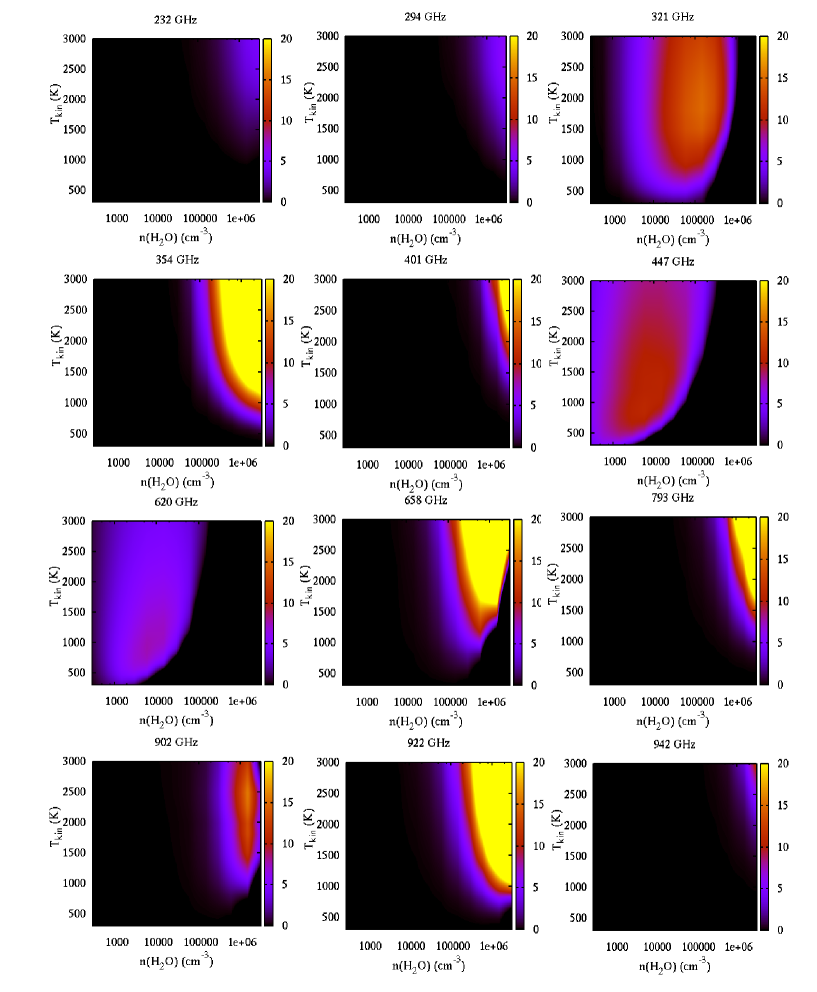
Figure 1: Maser depths (negative optical depths) for the lines of o-H₂O visible to ALMA in bands 3-10 as functions of kinetic temperature and o-H₂O number density. The maser depths are represented by a colour table that is the same for all transitions. These plots represent a sample of the parameter space of the model at a dust temperature of 50 K and zero velocity shift. Plots of the transitions at 826 and 848 GHz have been omitted: they resemble 232 GHz, but are even more extremely concentrated to the top-right-hand corner of the plane. Note that black indicates only that the transition is not inverted; the level of absorption is not displayed. As the water spin-species are treated independently, conversion of the $x$-axis to n(H₂) may be effected simply by dividing by the fractional o-H₂O abundance of 3$\times$10^-5.

The maser transitions plotted in Fig. 1 may be divided into two families on the basis of the region occupied by the positive maser depths in the $n_{\mathrm{H_{2}O}}$ versus $T_{K}$ plane. One family, comprising 321,447,620,658 and 902 GHz, have a peak maser depth within the region plotted, whilst the remainder, and the omitted 826 and 848-GHz lines have depths that are still rising at the maximum density and $T_{K}$ covered by the model.

These families of transitions are not simply a convenient classification based on the appearance of plots: they have a physical basis that reflects the excitation of the transitions involved. The first family all have an upper energy level less than 2600 K above ground, whilst the second family have upper state energies corresponding to at least 3100 K, and rising to 7165 K in the case of 395 GHz. The first family are therefore mostly pure rotational transitions, sited either within the ground vibrational state, or within the $v_{2}=1$ excited state, whilst the second family include rotational transitions in more highly excited vibrational states and a number of rovibrational transitions. At $T_{d}=$50 K, this is exactly what we expect: upper energy levels are populated almost entirely by collisions, so $T_{K}$ must be comparable to the upper-state energy, and high densities are favoured, increasing the collision rate until a critical density is reached that thermalises the populations and destroys any inversion.

Transitions for which the bulk of the inverted region is captured by the figure, for example 321, 447, 620 and 902 GHz, show a much steeper decay of the maser depth on the high-density side than on low-density side. This is evidence of a well-defined critical density, above which the energy levels in the transition become thermalized. However, it is apparent that the critical density depends quite strongly on the kinetic temperature, particularly when this is near the lower limit of the inverted range. The logarithmic density scale in the plots compresses this variation: the critical density at 321 GHz, for example, drops by a factor of 5 as the kinetic temperature falls from 1500 to 500 K.

In Fig. 2, we plot the p-H₂O counterpart to Fig. 1. Again, some transitions (137,488 and 832 GHz) have been omitted from the plot: they resemble the panel for 262 GHz, but are even more concentrated towards the high density and temperature regime; the most extreme transition in this respect is 488 GHz. There is also a similar division into low- and high-excitation families of lines, with the low-excitation family comprising the 183, 325, 474, 899, 906 and 916 GHz transitions and the high-excitation family, 96, 137, 209, 250, 263, 297, 488, 610 and 832 GHz.

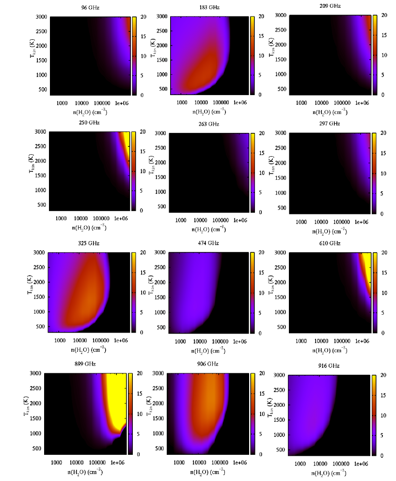
Figure 2: As for Fig. 1, but for p-H₂O. Plots of the transitions at 137, 488 and 832 GHz have been omitted: they resemble 262 GHz, but are even more extremely concentrated to the top-right-hand corner of the plane. As the water spin-species are treated independently, conversion of the $x$-axis to n(H₂) may be effected simply by dividing by the fractional p-H₂O abundance of 3$\times$10^-5.

Fig. 3 and Fig. 4 are the respective analogues of Fig. 1 and Fig. 2 in the range of frequencies accessible to SOFIA.

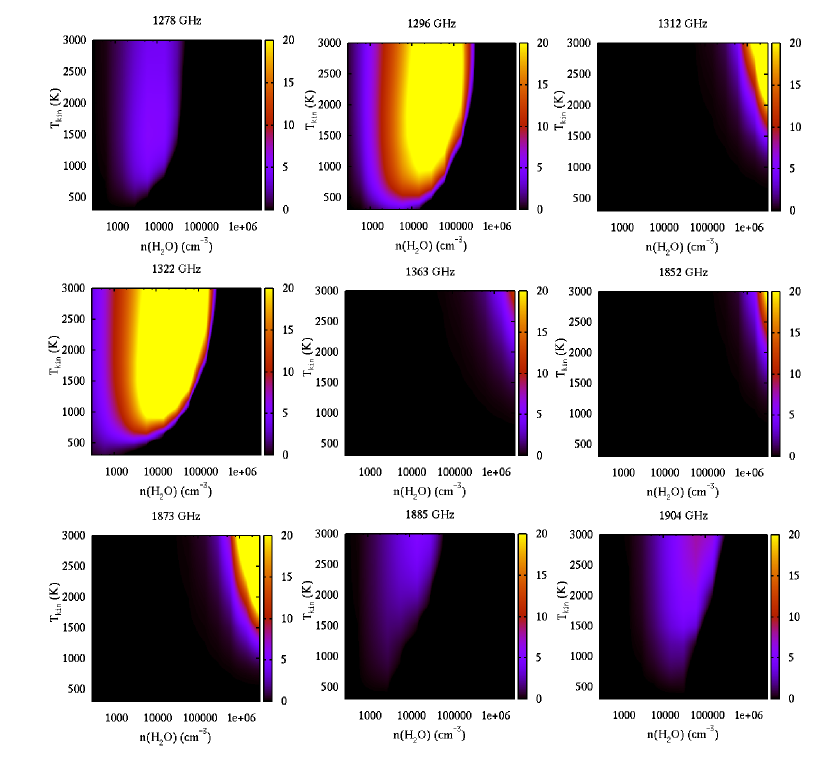
Figure 3: As for Fig. 1, but for o-H₂O transitions accessible to SOFIA. Plots of the transitions at 1459,1478,1491 and 1816 GHz have been omitted: they resemble 1363 GHz plot, but the inverted region is more extremely concentrated to the top-right-hand corner of the plane.

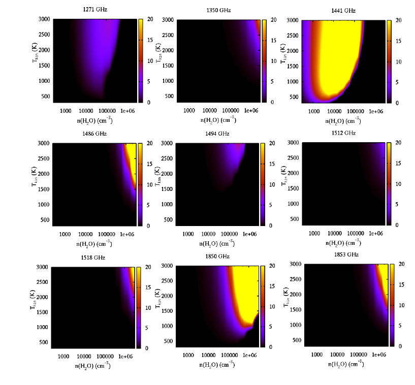
Figure 4: As for Fig. 1, but for p-H₂O transitions accessible to SOFIA.

The set of transitions visible to SOFIA contains a larger fraction of rovibrational transitions, and rotational transitions from vibrationally excited states, than the ALMA set, and there are consequently more lines without laboratory-measured frequencies and large frequency uncertainties, see Table 6.

Lastly in this section we plot, in Fig. 5, maser depths for three other maser lines from Table 6: 22, 67 (or 67.8) and 380 GHz. These lines are not detectable with ALMA in cycle 3, but 67 GHz may eventually become accessible when detectors for band 2 are constructed. The 380-GHz transition is in a position of strong atmospheric opacity, and is consequently a poor target for ground-based observations. Depth in the 22-GHz transition is plotted, since this is the most common water maser line; it will not be observable in future with ALMA unless the lower frequency of Band 1 is reduced below the current planned value of 31.3 GHz.

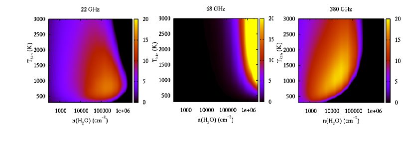
Figure 5: As for Fig. 1, but for some well-studied transitions not accessible to SOFIA or the cycle-3 configuration of ALMA.

4.1.1 Effect of dust

The models discussed so far have used $T_{d}=50$ K, so the pumping effect of radiation emitted by the dust is very weak. Here we discuss models where the dust temperature takes the values $T_{d}=1025$ K and $T_{d}=1400$ K (approximately the condensation temperature of several refractory elements, (Draine, 2011)), whilst the ranges of $T_{K}$ and water number density are the same as in Section 4.1. The numbers of transitions found to achieve a maser depth of at least $\tau=3.0$ at $T_{d}=1025$ K were 60 for o-H₂O and 30 for p-H₂O. At the level of $\tau=10.0$, these numbers reduced, respectively, to 31 and 20. Of the 60 o-H₂O lines recorded at $\tau=3.0$, 19 were not already recorded at $T_{d}=50$ K. The corresponding figure for p-H₂O was 18. These lines, strongly inverted only at the higher dust temperature, require a significant radiative contribution in their pumping. They have been added to Table 6, but may be easily identified by the frequencies printed in an Italic font. The effect of increasing the dust temperature is to progressively destroy the inversions in most of the prominent maser transitions found at $T_{d}=50$ K.

We plot the maser optical depths in the density/kinetic temperature plane for the additional o-H₂O transitions visible to ALMA in Fig. 6; a similar plot for the ALMA p-H₂O lines is presented in Fig. 7. The locus of inversion for many of the transitions in these plots is notably different from most transitions at $T_{d}=50$ K. The sole exception is 941 GHz, which resembles the very high temperature and density family found at $T_{d}=50$ K, for example 294 GHz in Fig. 1.

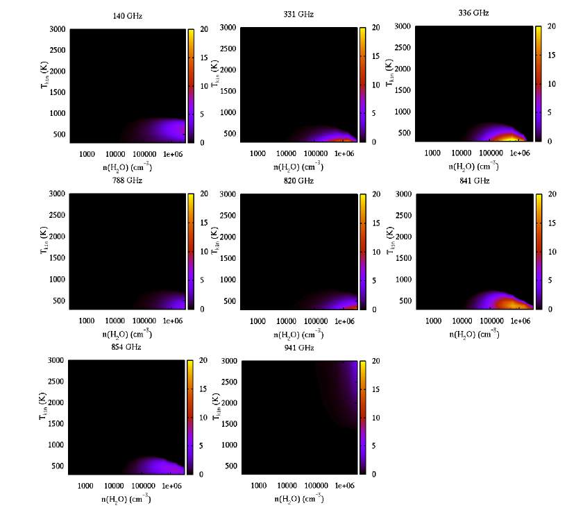
Figure 6: As for Fig. 1, but for transitions visible to ALMA that were found to be significantly inverted (maser depth $\geq$3) at a dust temperature of 1025 K, but not previously found at $T_{d}=50$ K. These transitions require a significant element of radiative pumping.

The remaining transitions have an inverted zone that is concentrated towards the bottom right-hand corner of each plot, corresponding to $T_{K}<800$ K and number densities of o-H₂O above 2$\times$10⁴ cm^-3. In four of the eight transitions the point of peak maser depth is apparently outside the plotted region at a temperature $T_{K}<300$ K. At this point, mention should also be made of the 268.15-GHz maser, discovered by Tenenbaum et al. (2010), that appears in Table 1: this transition narrowly missed our classification as a strong maser at $T_{d}=1025$ K, but would pass at higher dust temperatures, for example 1250 and 1400 K. If plotted in Figure 6, the distribution of its maser depth would closely resemble that of 820 GHz. A similar story was found for the potential ALMA p-H₂O transitions that are plotted in Fig. 7:

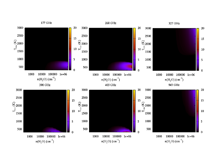
Figure 7: As for Fig. 2, but for transitions visible to ALMA that were found to be significantly inverted (maser depth $\geq$3) at a dust temperature of 1025 K, but not previously found at $T_{d}=50$ K. These transitions require a significant element of radiative pumping.

the transitions at 327 and 943 GHz have an inverted region similar to the high-excitation transitions at $T_{d}=50$ K, whilst the remainder resemble the typical radiatively pumped o-H₂O transitions in Fig. 6. The 943-GHz transition is the only rovibrational example in Fig. 7, and, followed by 327 GHz, has the highest upper state energy in the figure.

The new radiatively-pumped o-H₂O transitions visible to SOFIA all occupy the low-kinetic temperature and high density locus of the plane (see Fig. 8), following the majority of the radiatively-pumped ALMA transitions in this respect. Although there is a sample of only three displayed transitions, the maser depth in the ground-state transition at 1308 GHz occupies a zone of the density/kinetic temperature plane at a substantially lower density than the 1358 and 1361-GHz transitions, which are both fully rovibrational: they have $(0,2,0)$ as a common lower vibrational state, with $(0,0,1)$ (asymmetric stretch) as the upper state of 1358 GHz and $(1,0,0)$ at 1361 GHz.

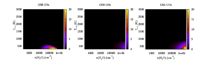
Figure 8: As for Fig. 6, but for transitions visible to SOFIA.

Maser depths for the radiatively pumped p-H₂O transitions visible to SOFIA are shown in Fig. 9.

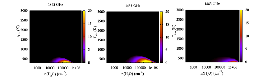
Figure 9: As for Fig. 7, but for transitions visible to SOFIA.

Both 1345- and 1435-GHz transitions are from the vibrational ground state, whilst the 1483-GHz transition is rovibrational, with an upper level 5722 K above ground in the asymmetric stretching mode $(0,0,1)$, transferring to a lower level in $(1,0,0)$. The locus of highest maser depth for this transition does appear to lie to the higher density side of those for the ground-state lines, but the effect is less pronounced than in the case of the o-H₂O transitions.

The number of inverted transitions in both o-H₂O and p-H₂O (above a threshold maser depth of 10) passes through a minimum at a dust temperature of approximately $T_{d}=650\,K$. When the dust temperature reaches 1025 K, as in the models discussed in detail above, 29 of the original 31 o-H₂O maser transitions (from $T_{d}=$50 K) no longer reach the threshold, but have been replaced by 30 radiatively pumped transitions. By the time the dust temperature reaches 1400 K, all the original lines have been lost, except 22 GHz, which has faded and then reappeared at 1250 K. Very few maser transitions share this property of having both collisional and radiative pumping systems (see below). The overall number of inverted transitions continues to rise with dust temperature. At $T_{d}=1400$ K, 25 new o-H₂O transitions have appeared above the threshold that were not present at 1025 K. The situation is similar for p-H₂O: at 1025 K only 2 of the original 23 (at $T_{d}=50$ K) transitions still reach the threshold, and all have been lost at $T_{d}=1400$ K. However, the transitions at 96, 209 and 324 GHz returned, having a radiative branch to their pumping mechanisms, as for 22 GHz (see above). At $T_{d}=1400$ K, 39 transitions were found above the threshold maser depth and, of these, 23 were not previously found at 1025 K.

We now consider the effect of continuously varying the dust temperature over a wide range for a restricted number of values of the kinetic temperature. For the moment, the velocity shift is fixed at zero, and other variables have their standard values. To represent as much information as possible graphically, we use a particular symbol to represent each transition, as specified in the key to each diagram. We then plot the maximum maser optical depth found in the data as a function of the dust temperature, $T_{d}$. The extra information, provided via the colour of each symbol, is the number density of H₂O at which the maximum maser depth was found.

In Fig. 10 (top panel), we plot the effect of increasing dust temperature on the inversions of o-H₂O maser lines at $T_{K}=471.43$ K, with frequencies below 400 GHz visible to ALMA. There are two families of lines: 321, 355 and 395 GHz are rather weakly affected by increasing dust temperature, and the effect is deleterious. These lines also have the density of peak inversion somewhere below 10³ o-H₂O molecules per cubic centimetre. By contrast, the remaining transitions broadly follow the pattern of 140 GHz, which is not inverted at $T_{d}=50$ K, but becomes inverted above $T_{d}=500$ K, with increasing maser depth thereafter. These transitions have a strong radiative component to their pumping scheme. Moreover, as the inversions increase, this family of lines generally has a density of peak maser depth that is at, or very close to, the maximum available in the model, that is above 10⁶ o-H₂O cm^-3. Obviously the highest values of $T_{d}$ plotted are physically unlikely, being above the sublimation temperature of most likely minerals, but are shown to illustrate the effect of a very strong infra-red field.

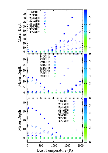
Figure 10: Maximum maser depths (negative optical depths) as a function of dust temperature for o-H₂O transitions with frequencies below 400 GHz visible to ALMA. From top to bottom, the kinetic temperatures for the three panels are 471.43, 985.71 and 1500.00 K. Colours of the symbols represent the o-H₂O number density at which the maximum maser depth was found. The colour scale is the log to the base 10 of the number density.

The lower panels in Fig. 10 represent slices through the parameter space at higher kinetic tempeatures (985.71 K and at the bottom, 1500 K). The main effect of increasing the kinetic temperature is to reduce the inverting effect of the dust radiation. At 1500 K, only the 140-GHz transition still shows a significant increase in maser depth at the higher dust temperatures. Inversions are weakened or destroyed in the other lines.

Figure 11 has the same layout at Fig. 10, but is for maser transitions with frequencies above 600 GHz. In this case, there are four strongly radiatively pumped lines at $T_{K}=471.43$ K: 788, 820, 841 and 854 GHz, with large maser depths in these lines appearing at $T_{d}>700$ K. The remaining transitions are weakly inverted at this kinetic temperature, and little affected by dust radiation. The lines that are radiatively pumped all achieve their maximum maser depths at densities at, or close to, the largest studied in the model. The same radiatively pumped group is evident at $T_{K}=985.71$ K (middle panel) but with somewhat reduced maser depths, that increase significantly beyond a dust temperature of $T_{d}>1300$ K. Large inversions are evident at $T_{d}<500$ K at 658, 794 and 923 GHz, and it is clear that inversions in these transitions are destroyed by radiation. The lower panel, for which $T_{K}=1500.00$ K shows no transitions being significantly pumped by the dust radiation. As in the middle panel, large inversions at 658, 794 and 923 GHz are destroyed by the radiation, whilst 941 GHz shows a peak maser depth at $T_{d}\sim 800$ K.

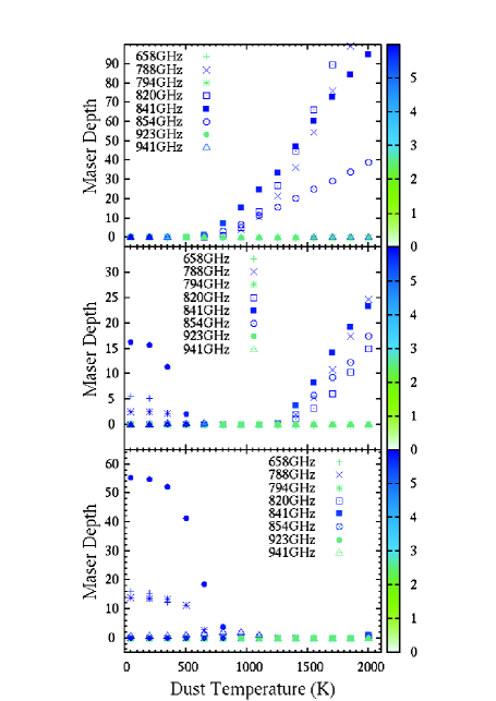
Figure 11: Maximum maser depths (negative optical depths) as a function of dust temperature for o-H₂O transitions with frequencies above 600 GHz visible to ALMA. Kinetic temperatures and symbol colours are as in Fig. 10.

Maser depths for transitions in p-H₂O are shown in Fig. 12 and Fig. 13. The former figure is for transitions with frequencies up to 325 GHz, and the latter, for transitions at higher frequencies, beginning with 327 GHz. At the lowest kinetic temperature of 471.43 K (top panel, Fig. 12), the 183- and 325-GHz masers initially decay with increasing dust temperature, reaching negligible inversion at around $T_{d}=500$ K. However, whilst the inversion at 183 GHz remains close to zero for higher values of $T_{d}$, the 325-GHz transition clearly has a radiatively-pumped branch at high density, since the triangular symbols begin rising again from about $T_{d}=1250$ K, reaching a maser depth of 8.9 at $T_{d}=2000$ K. This behaviour is shared with the well-known o-H₂O transition at 22 GHz (see below). For 325 GHz, the radiative branch only appears at the lowest kinetic temperature: it is not repeated in the two lower panels, where gain at 325 GHz only decays with rising $T_{d}$. At the lowest kinetic temperature (top panel) four of the other transitions that appear are radiatively pumped. Like the o-H₂O maser transitions in Fig. 10 and Fig. 11, the radiative pumping becomes strong above $T_{d}\sim 700$ K, and it is strongest for 96 GHz, with decreasing maser depth through 260, 209 and 177 GHz. The radiatively pumped lines also have their peak maser depth at, or near to, the maximum available water density - a property that is also shared with the o-H₂O lines. The remaining two transitions, at 250 and 297 GHz, have small maser depths over the full range of dust temperature.

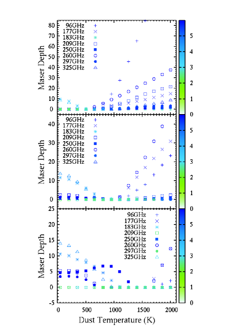
Figure 12: Maximum maser depths (negative optical depths) as a function of dust temperature for p-H₂O transitions with frequencies up to, and including, 325 GHz visible to ALMA. Kinetic temperatures and symbol colours are as in Fig. 10.

As the kinetic temperature is increased to $T_{K}=985.71$ K (Fig. 12 middle panel), we see a reasonably simple modification of the upper panel: the radiatively pumped transitions achieve lower maser depths, and begin rising beyond a higher dust temperature of about 1000 K. The 209-GHz transition, though weakly masing throughout, now behaves somewhat like the 325-GHz transition in the upper panel, with evidence of both collisional and radiative pumping. At $T_{K}=1500$ K, 96, 177 and 260 GHz remain the only radiatively pumped transitions; the remainder decay with increasing dust temperature, although 250 GHz shows a weak maximum in maser depth at $T_{d}\sim 800$ K.

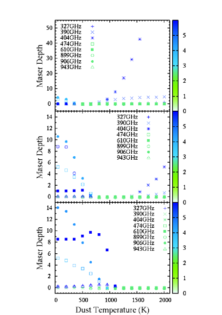
Figure 13: Maximum maser depths (negative optical depths) as a function of dust temperature for p-H₂O transitions with frequencies above 325 GHz visible to ALMA. Kinetic temperatures and symbol colours are as in Fig. 10.

In Fig. 13, the higher frequency p-H₂O transitions break neatly into two families: those at 403, 390 and 327 GHz are radiatively pumped, though for 327 GHz, the effect is rather weak. As in previous graphs, the effect of radiative pumping falls with increasing kinetic temperature, and there is no significant gain left in any of these lines at $T_{K}=1500$ K (bottom panel). The other seven transitions are predominantly collisionally pumped, and mostly become stronger as $T_{K}$ rises. Maxima appear in the curves for the 610 and 943-GHz transitions at respective dust temperatures of 650 and 800 K in the bottom panel.

We now consider transitions visible to SOFIA. The general separation into collisionally and radiatively pumped families of lines is very similar to the behaviour observed at lower frequencies, and the number of transitions is small enough that the most important can be studied through one graph each for the o-H₂O and p-H₂O lines. The response of the maser depth in eight transitions o-H₂O to variation of the dust temperature is plotted in Fig. 14. As for the ALMA transitions, results are plotted for three different kinetic temperatures, with $T_{K}$ increasing from the top to the bottom panel.

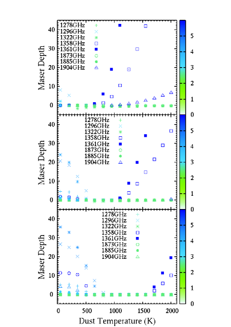
Figure 14: Maximum maser depths (negative optical depths) as a function of dust temperature for o-H₂O transitions visible to SOFIA. Kinetic temperatures and symbol colours are as in Fig. 10.

Five of the transitions shown, namely 1278, 1296, 1322, 1873 and 1885 GHz, are clearly collisionally pumped: their maser depths fall with increasing $T_{d}$, become more powerful with increasing $T_{K}$, and their maximum depths are often found at a modest number density of typically 10³-10⁴ o-H₂O cm^-3. The two transitions at 1358 and 1361 GHz are radiatively pumped, showing maser depth rising with $T_{d}$, but generally falling with $T_{K}$; the maximum maser depth is found at or near the highest number density in the model. Previously noted effects for radiatively pumped lines also apply here: there is a critical dust temperature for significant maser depth of typically $T_{d}=700$ K in the top panel (where T_K=471.43 K), but increasingly delayed to higher $T_{d}$ as we progress towards the bottom panel (higher T_K). The 1904-GHz transition displays a more peculiar behaviour, appearing to be radiatively pumped in the top panel, but collisionally pumped at $T_{K}=985.71$ and 1500 K.

The variation of maser gain with $T_{d}$ for eight p-H₂O transitions visible to SOFIA is shown in Fig. 15.

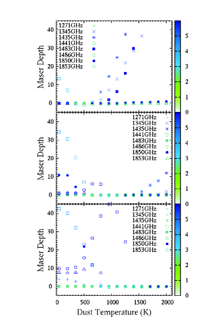
Figure 15: Maximum maser depths (negative optical depths) as a function of dust temperature for p-H₂O transitions visible to SOFIA. Kinetic temperatures and symbol colours are as in Fig. 10.

The major oddity in this case is the 1486-GHz transition. Although not significantly inverted at $T_{K}=471.43$ K, the maser depth in this line shows a maximum as a function of $T_{d}$ at both the higher kinetic temperatures. The effect is particularly strong at $T_{K}=1500$ K (bottom panel) where the peak maser depth occurs at $T_{d}=950$ K. Higher dust temperatures result in a very rapid decline in the inversion. The transition shares with radiatively pumped lines the property of having maximum maser depths associated with very high number densities. A weak maximum also appears for 1853 GHz, but it is perhaps best to consider this as a collisionally pumped transition (along with 1271, 1441 and 1850 GHz). The transitions at 1345, 1435 and 1435 GHz exhibit typical radiatively pumped behaviour, but none remain in the bottom panel.

4.1.2 Effect of velocity gradient

The discussion so far has considered results from slabs without a velocity gradient. We now consider the effect of introducing positive and negative velocity gradients through the slab. In a slab with a velocity gradient that is defined as positive in this work, an observer situated on the optically thin (observer’s) side of the slab would see material approaching faster at each successive depth point towards the optically thick boundary. Radiation from the most remote layers therefore appears more blue shifted. In a slab with a negative velocity gradient, it is the outermost layers that approach the observer fastest, and radiation from more distant slabs is progressively redshifted. A typical AGB star envelope, for example, would have a negative velocity gradient in this scheme, except for its innermost shock-dominated zone. The velocity gradients are constant over the model, so that the velocity shift varies linearly with depth; velocity variation is therefore concentrated in the geometrically thicker slabs. In most of the results presented in this section, only the total velocity shift through the model is considered.

When considering variation of inversion, or maser depth, with velocity shift, we would ideally hold all other parameters at some set of standard values. However, from the variation with dust temperature, studied in Section 4.1.1 above, we can see that there is no good single choice of $T_{d}$: we need at least two, one to represent typical conditions for collisionally pumped transitions, and a second, higher, value for those transitions that are predominantly radiatively pumped. The value of $T_{d}=1025$ K, specified as standard in Table 3 is suitable for the radiatively pumped transitions, but we also use $T_{d}=350$ K as representative of collisionally-pumped transitions.

Radiatively pumped transitions also tend to show their largest maser depths at low kinetic temperatures compared to the collisionally pumped subset. It is therefore also impossible to choose a single representative value of $T_{K}$, and we use the same three values as in Section 4.1.1. The overall result is that we display variation of maser gain for groups of transitions in blocks of 6 graphs, corresponding to 2 values of $T_{d}$, and 3 of $T_{K}$.

The first plot of this type is Fig. 16 for the group of o-H₂O masers visible to ALMA, with frequencies below 400 GHz, as considered for the effect of $T_{d}$ in Figure 10.

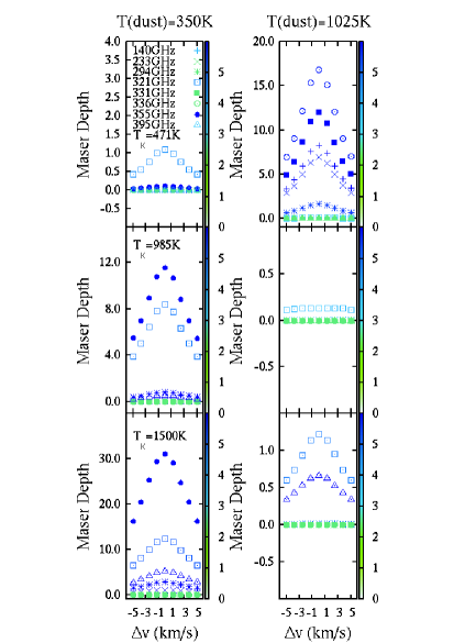
Figure 16: Maximum maser depths (negative optical depths) as a function of velocity shift at 3 kinetic and 2 dust temperatures. Kinetic temperature increases downwards, and is the same for any pair of panels horizontally; the value is marked in the left-hand panel of each pair. Panels in a given column share the same dust temperature, with the value marked at the top of the column. Maser transitions are identified by the symbols listed in the key that appears in the top-left-hand panel only. The colour of a symbol, in any panel denotes the base-10 logarithm of the o-H₂O number density at which the maximum maser depth was found, as in Section 4.1.1. The colour palette appears to the right of each panel.

Perhaps the main result is that, at least for this subset of powerful maser transitions, the effect of velocity shifts are close to symmetric about $\Delta v=0$. For large maser depths, the effect of increasing $|\Delta v|$ is always deleterious. We also see that the contrast, $\tau_{0}/\tau_{5}$, where $\tau_{0},\tau_{5}$ are the respective maser depths at $\Delta v=0$ and $\Delta v=5$ generally increases with $\tau_{0}$. We consider some of these statistics more quantitatively below. It is also apparent that, for all velocity shifts, high maser depth correlates with high number density of water (darkest blue colours), whilst green symbols (low density) are associated with weak gain or absorption across all velocity shifts. These conclusions are unchanged in general terms for the set of o-H₂O transitions with frequencies above 400 GHz, displayed in Fig. 17.

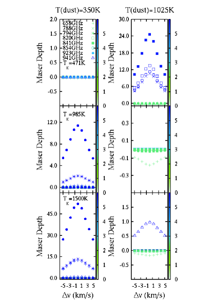
Figure 17: As for Fig. 16, but for a group of o-H₂O transitions with rest frequencies $>$400 GHz.

The higher frequency transitions are almost completely inactive, at all velocity shifts, in the top-left panel (T${}_{K}=350$ K and T${}_{d}=1025$ K. The appearance of modest inversions at 321,395 and 941 GHz in bottom right-hand panels suggests that these transitions may be pumped both collisionally and radiatively.

The effect of velocity shifts on the strongest ALMA maser transitions of p-H₂O is shown in Fig. 18 and Fig. 19.

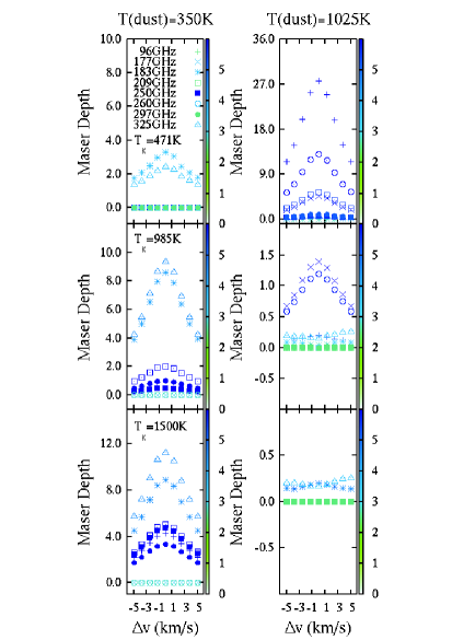
Figure 18: As for Fig. 16, but for a group of p-H₂O transitions with rest frequencies $\leq$325 GHz.

In Fig. 18, we see for the first time evidence of strongly asymmetric behaviour of maser depth with velocity shift. This occurs in the right-hand ($T_{d}=1025$ K) column, and the two lower panels at $T_{K}=$985 and 1500 K. In both these panels, the 325-GHz maser depth is largest at $\Delta v=5$ km s^-1, and weakest for zero velocity shift. However, in both cases the maser depth in this transition is small, reaching only 0.25. At 985 K, the even smaller maser depth at 183 GHz is close to symmetric, but smallest at zero shift.

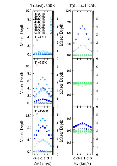
Figure 19: As for Fig. 16, but for a group of p-H₂O transitions with rest frequencies $>$325 GHz.

There is no similar behaviour in Fig. 19, which covers the strongest p-H₂O maser transitions with frequencies above 325 GHz. There is evidence for weak radiative pumping at 610 GHz and a strong correlation between maser activity and high number density in the right-hand column.

The effect of velocity shift on the strongest o-H₂O maser transitions visible to SOFIA is shown in Fig. 20.

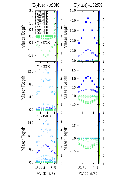
Figure 20: As for Fig. 16, but for a group of o-H₂O transitions suitable for observations with SOFIA.

The top left-hand panel of Fig. 20 shows the strongest absorption found for any of the transitions plotted in Figures 16-21: it is in the transition at 1322 GHz. The effect of velocity shift on this absorption is, however, close to symmetric as for most inverted transitions. An increase of kinetic temperature to 985 K is enough to transform the 1322-GHz absorption to a large positive maser depth (middle left panel), and this has become the strongest maser transition at $T_{K}=1500$ K (bottom left panel). At high kinetic and dust temperature (bottom right-hand panel), there is some absorption, but little or no maser activity, suggesting that none of the transitions plotted in Fig. 20 are both collisionally and radiatively pumped. As noted previously, at the higher dust temperature particularly, strong maser action correlates with high density.

The final set of plots of this type, Fig. 21, for selected strong p-H₂O transitions visible to SOFIA, shows a significant absorption asymmetry at 1441 GHz in the top-right panel, where the most negative maser depth is at a shift of -1 km s^-1, rather than at zero. There is also a noticeable variation in the density of maximum absorption as a function of velocity shift in this transition. The 1441-GHz transition is inverted at the higher temperatures in the left-hand panels, but is also quite strongly absorbing at $T_{d}=1025$ K and $T_{K}=985$ K (middle right-hand panel), where the strongest absorption is at zero shift. The 1486-GHz transition is strongly inverted in both bottom panels, and is therefore likely to have both collisional and radiative pumping schemes.

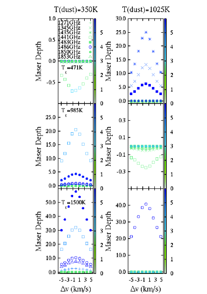
Figure 21: As for Fig. 16, but for a group of p-H₂O transitions suitable for observations with SOFIA.

For a more quantitative discussion of asymmetry and contrast, we define the following pair of statistics: the asymmetry parameter is

$$q_{a}=\sum_{i=1}^{4}(\tau(\Delta v_{i})-\tau(-\Delta v_{i}))/\tau(0),$$ (2)

where the sum is over the positive non-zero velocity shifts, and $\tau$ represents the maser depth at the specified shift or $\tau(0)$ for zero shift. A systematic trend of larger maser depths at positive shifts yields a positive value of $q_{a}$; a perfectly symmetric distribution gives $q_{a}=0$. The contrast parameter is

$$q_{c}=2\tau(0)/(\tau(5)+\tau(-5)),$$ (3)

which is the ratio of the maser depth at zero shift to the mean of the depths at the largest positive and negative shifts. Results are discussed below for the 48 transitions plotted in Fig.16-Fig21. In some cases, a statistic is given in terms of the six panels in which the transition appears, whilst in other cases, the average over the six panels only is considered.

Of the 48 transitions, 31 have a negative mean asymmetry and 17 positive. The line with the strongest negative asymmetry on average is 233 GHz with $q_{a}=-0.5525$; the strongest positive asymmetry is in 325 GHz with $q_{a}=0.3417$. Both results are dominated by panels with rather weak maser depths. The transitions with the smallest (largest) mean contrast is 331 GHz with $q_{c}=0.8385$ (1486 GHz with $q_{c}=2.1463$). It may be more instructive to consider maximum and minimum values that relate to individual panels in Fig.16-Fig21, rather than to averages over the 6 panels in which data is plotted for a particular frequency. At this level of detail, the greatest positive asymmetry is $q_{a}=1.9391$ for 294 GHz, middle right-hand panel, Fig. 16, and the greatest negative asymmetry is $q_{a}=-3.5148$ at 233 GHz, again in the middle right-hand panel of Fig. 16. Both of these extremes correspond to distributions where the maser depths are $\ll$1. The greatest contrast is $q_{c}=2.5348$ at 321 GHz (Fig. 16, top left-hand panel) and the weakest for an inverted transition is $q_{c}=0.0435$ (bottom right-hand panel of the same figure, but for 140 GHz). Whilst the weakest contrast is again found under conditions where the maser depth is $\ll$1, the strongest is associated with a modest maser depth of $\tau\simeq 1$ at zero shift.

The limited effect of velocity fields that is evident in the discussion above also extends to transitions that do not appear in Fig.16-Fig21, but is not negligible. Lists of o- and p-H₂O transitions with maximum maser depth $>$3 were prepared for $T_{d}=1025$ K and $T_{d}=350$ K and velocity shifts of zero and both $\pm$5 km s^-1. It is important to note that these maximum maser depths were found with respect to number density and kinetic temperature, rather than number density and velocity shift (as represented by the symbol colours in Fig.16-Fig21). Lists at $\pm$5 km s^-1 never contained new maser transitions that were not already present at zero velocity shift. In fact, the lists at higher shifts were generally substatially shorter than those at zero shift. However, the effects of introducing a velocity shift were not found to be negligible, since, in every case examined, a small subset of transitions were found to have a larger maximum maser depth at one or both of the extreme shifts than the maximum found for zero shift. For o-H₂O at $T_{d}=1025$ K, the 140,1308 and 1359-GHz transitions (3 of 20 strong masers at $\Delta v=-5$ km s^-1) had larger maxima than at zero shift. In this case, the same set of transitions also had higher maxima at $\Delta v=+5$ km s^-1. At $T_{d}=350$ K, 11 of 21 strong masers at $\Delta v=-5$ km s^-1 had higher maxima than at zero shift (321,658,556,902,793,1739,1321,1295,1694,1643 and 1538 GHz). The 1295-GHz transition was lost from this list at $\Delta v=+5$ km s^-1. A broadly similar set of results was found for p-H₂O: 6 of 16 strong masers had larger maximum depths at $\Delta v=-5$ km s^-1 than at zero shift for $T_{d}=1100$ K (96,1109,1486,1478,1435 and 1407 GHz). The 1109 and 1478-GHz lines were not included at $\Delta v=+5$ km s^-1. At $T_{d}=35$ K, 7 of 15 transitions had an enhanced maximum at $\Delta v=-5$ km s^-1: 533,905,899,592,1077,1440 and 1849 GHz). This list was the same, bar the loss of 899 GHz at $\Delta v=+5$ km s^-1. Plots were made of the contrast as a function of maser depth at zero shift for several lines individually and for all lines together, but no simple relationship was apparent.

4.1.3 Effect of microturbulence and dust modelling

In this section we briefly discuss some test models where input parameters have been varied significantly away from their standard values or formulas. Specifically, we consider the effect of varying the microturbulent speed, changing the size distribution of the dust, and artificially limiting the effects of line overlap.

The microturbulent speed is one of the standard cloud variables, and is used as a temperature-independent line-broadening parameter only. We consider its effect on a small subset of maser transitions for the standard, and four additional values. The results are shown in Table 4. For the standard values of the other cloud variables, see Table 3.

Table 4: Effect of microturbulent speed on maser depth

	$v_{T}$(km s-1)
	0.0	1.0	2.0	3.0	4.0
$\nu$(GHz)
22	1.5533	1.3019	0.9768	0.7620	0.6232
68	0.8378	0.6309	0.4032	0.2781	0.2071
321	2.3217	1.8155	1.2112	0.8534	0.6402
380	1.2271	1.0040	0.7242	0.5517	0.4434
448	1.6629	1.3013	0.8327	0.5493	0.3857
595	0.2536	0.1554	0.0567	0.0117	-0.0075
658	-13.113	-10.546	-7.4581	-5.5634	-4.4021
1361	-3.8623	-3.0824	-2.1547	-1.6060	-1.2720
96	-0.6384	-0.4899	-0.3195	-0.2226	-0.1672
183	2.0100	1.6156	1.1314	0.8459	0.6760
325	0.4698	0.4186	0.3581	0.3100	0.2762
474	0.4509	0.1923	-0.0356	-0.0973	-0.1019
547	0.6922	0.4810	0.2569	0.1460	0.0907
609	0.1189	0.0810	0.0426	0.0246	0.0158
906	-0.1061	-0.0572	-0.0446	-0.0554	-0.0655
1435	-5.7881	-4.5243	-3.0364	-2.1662	-1.6518

The principal effect of the microturbulent speed is to lower the maser depth of inverted transitions as $v_{T}$ is increased; this is in accord with expectations, since increasing $v_{T}$ reduces the optical depth in pumping transitions. Even the collisional scheme suffers from this effect, since radiative processes are required to couple the backbone levels (see Section 1.5). Transitions that are in absorption (negative depths in Table 4) also lose absorbing power with increasing $v_{T}$, as shown by the entries for 658 and 1361 GHz. The rows for 595 GHz and 474 GHz show that weakly inverted transitions under standard conditions can be forced into weak absorption by increasing $v_{T}$ to 4 km s^-1. A differential effect is demonstrated (amongst other transitions) by the 380- and 448-GHz rows: 448 GHz has the larger maser depth at $v_{T}=0$ km s^-1, but the 380 GHz depth is the larger for $v_{T}>3$ km s^-1. At 906 GHz, a weakly absorbing transition at $v_{T}=0$ initially becomes still more weakly absorbing as $v_{T}$ increases. However, it does not pass into inversion, but the absorbing strength passes through a minimum between $v_{T}=2$ and 3 km s^-1, beyond which the absorbing power again increases.

We test the robustness of the dust model by moving from the spectrum of sizes with upper and lower limits, as introduced in Section 3, to monodispersed dust, where the single grain radius is equal to the mean radius of the original distribution ($\bar{a}=1.667$ nm). The dust mass fraction and opacity behaviour with wavelength were as used in the main model. We present the results for four maser transitions of p-H₂O in Fig. 22, plotting maser depths as a function of dust temperature for the standard (black symbols) and monodispersed models (red symbols). Other input parameters were as in Table 3, except that $T_{K}=1500$ K was used instead of $1750$ K, because more data were available at the lower temperature.

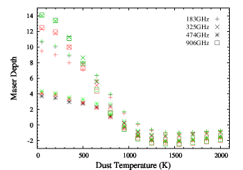
Figure 22: Maser depths in 4 maser transitions of p-H₂O as a function of dust temperature. Other physical conditions are standard, except that $T_{K}=1500$ K. Colours denote the usual model (black), monodispersed dust (red) and no line overlap (green).

It can be seen that changing to a monodispersed dust model typically changes the maser depths by a few per cent, but does not change the general trend of strong masers falling into absorption as $T_{d}$ is increased. For three of the transitions shown, the standard model has generally higher maser gains for a given $T_{d}$, but maser depths are more positive in the monodispersed model at 474 GHz.

We also plot in Fig. 22 (green symbols) results for a model that uses the standard dust, but has no line overlap. This restriction was imposed by limiting the size of overlapping groups to a maximum of 1, so that all transitions have (artifically) independent line shapes. For the transitions in Fig. 22, results are also generally modest differences from the standard model. At 905 GHz, omission of line overlap slightly depresses the maser depths and reduces absorption at higher values of $T_{d}$. However, at the other three frequencies, maser depths are somewhat larger without overlap. A more quantitative effect appears in the 471-GHz transition, which is weaker than the plotted lines under these conditions: in the standard model this line has a maser depth of 2.19 at $T_{d}=50$ K (2.53 with monodispersed dust), but without line overlap the transition is in absorption (maser depth -0.094). In the overlap-free model, the 471-GHz transition is only very weakly inverted at $T_{d}=350$ and $500$ K, rather than being continuously inverted over the range $T_{d}=50-800$ K.

4.2 AGB Stars

We have seen in Section 1.6 that the scale size of maser clouds is expected to be approximately proportional to the radius of the host star. The results discussed up to this point are all based on slabs of thickness 2.25$\times$10¹⁴ cm, considered appropriate for a red supergiant star, such as VY CMa (see Section 3). We now briefly discuss the effect of reducing the cloud thickness to something more appropriate for the extended atmosphere of an AGB star, namely 4.5$\times$10¹³ cm.

Only two slab thicknesses have been considered, so we tabulate the effect of changing scale for a number of transitions of both spin species of H₂O. We choose conditions where each transition is a reasonably strong maser for the thicker slab, so the selected water number density, $T_{K}$, $T_{D}$ and corresponding maser depths are listed for each transition. Velocity shift is zero in all cases and the constant microturbulent speed is 1 km s^-1. Results are tabulated in Table 5. Note that $T_{K}$ is limited to a maximum of 1500K, since this was the maximum value used for the thinner slab.

Table 5: The effect of changing slab thickness on maser depths achieved for selected strong maser transitions; $R$ is the ratio of the maser depth in the thick (supergiant) model to the depth in the thin (AGB star) model.

$\nu$	$n_{H{{}_{2}}O}$	$T_{K}$	$T_{d}$	$\tau_{SG}$	$\tau_{AGB}$	$R$
(GHz)	cm-3	K	K
22	1.5(5)	814	50	15.45	2.624	5.888
321	6.0(4)	1500	50	13.35	2.676	4.989
336	3.0(5)	471	1025	12.82	1.869	6.859
380	3.0(6)	1500	50	33.85	6.424	5.269
447	6.0(3)	900	50	10.79	2.843	3.795
658	6.0(5)	1500	50	15.90	2.971	5.352
841	6.0(5)	471	1025	24.62	3.774	6.524
902	1.5(6)	1500	50	11.47	2.267	5.060
922	3.0(6)	1500	50	55.26	7.000	7.894
1296	3.0(4)	1500	50	26.59	5.785	4.596
1308	1.5(5)	471	1025	12.61	1.682	7.497
1322	1.5(4)	1500	50	35.67	8.047	4.433
1361	3.0(6)	471	1025	42.42	5.743	7.386
183	3.0(4)	1071	50	11.56	3.159	3.659
260	3.0(6)	557	1025	15.69	2.587	6.065
325	3.0(4)	1329	50	14.17	3.676	3.855
403	1.5(6)	300	1025	25.92	3.395	7.635
899	1.5(6)	1500	50	45.70	9.131	5.005
906	3.0(4)	1500	50	14.12	3.657	3.861
1441	3.0(4)	1500	50	42.61	10.06	4.236
1850	1.5(6)	1500	50	63.96	0.000	$\infty$

The supergiant slab is geometrically five times thicker than the AGB slab. For a constant and equal gain coefficient throughout both slabs, we would naively expect that the ratio of maser depths would be close to 5.0 for any line, with deviations due to more subtle radiative transfer effects. With the exception of the 1850-GHz transition of p-H₂O, which is not inverted in the thinner model, all examples of the ratio $R$ are indeed within a factor of 2 of the naively expected value. For the listed transitions of o-H₂O, the mean value of $R$ is 5.811 with a standard deviation of 1.306. For the p-H₂O transition, excluding 1850 GHz, the corresponding figures are 4.902 and 1.472. The grand average is 5.493 with a standard deviation of 1.400.

5 Predictions for Observations

Our list of predicted maser lines from zero frequency to 1910 GHz is presented in Table 6. The typeface in column 1 indicates whether the transition is predominantly pumped by collisions or radiation. Column 9 indicates whether the maser is potentially observable in one of the ALMA or SOFIA bands or, for lower frequency transitions, the radio band in which the maser might be observed with a different ground-based instrument. The final column gives the expected ratio of the maximum maser depth in the transition to the maximum found at 22 GHz. A couple of caveats should be observed regarding this ratio: firstly, the figure takes no account of saturation, so numbers significantly greater than 1 would not be reflected in brightness ratios of observed masers; secondly, under the conditions where the radiative transitions were added ($T_{d}=1025$ K), 22-GHz is not a strong maser, so its depth at $T_{d}=50$ K was used, and the maser depths are therefore not compared under the same radiation field. Kinetic temperatures for the two maser depths could be different for all transitions.

It is arguably more informative to attempt to predict which maser lines are closely associated with each other, and under what conditions. There are various reasonable ways to attempt this: one idea is a points-based pair-wise correlation function. This has the advantage of relatively simple visual presentation, and more complex groupings can reasonably easily be constructed from it. However, the exact number of points to award for, for example, finding two maser transitions with potentially saturating maser depths under the same physical conditions, is open to much debate. We therefore defer the construction of such a function to future work.

A more qualitative picture can be deduced from examining the groupings that we have already found. Grouping of transitions by pumping scheme has been discussed in detail in Section 4.1.1, and collisionally and radiatively pumped transitions may be identified in Table 6. The transitions that have both radiative and collisional branches in their pumping schemes (22,96,209,321,325,395,941 and 1486 GHz) may be problematic in the analysis of observational data, since they may have unusual, or previously unexpected spatial association with other transitions.

Based on the loci of inverted regions in the number-density/kinetic temperature plane, we can perhaps group the masers displayed in Fig. 1-Fig. 5 into four families: firstly the ‘classic’ set, comprising 321,906,1271,1278,1296,1322,1441,1885 and 1904 GHz. These masers have a collisional pump, with a peak maser depth reasonably close to $T_{K}=1500\,K$ and $n_{H_{2}}=10^{9}$ cm^-3. The 22-GHz transition is shared between this group and the ‘low-temperature’ set (183,325,380,447,474,620 and 916 GHz), which form at a number density close to, or rather below, that for the classic set, and at $T_{K}\sim 1000$ K. A third group, with 658 GHz as the typical member, comprising 658,902,899 and 1850 GHz, have a peak maser depth associated with $T_{K}\sim 2500$ K or higher, but with a number density that is substantially lower than the maximum used in the model, perhaps of order 10¹⁰ cm^-3. The remaining transitions form a fourth, hot, dense, group that has a peak maser depth at a density and kinetic temperature beyond the top right-hand corner of the plotted plane.

Masers with a predominantly radiative pump add three transitions, 327,941 and 943 GHz to the hot, dense group above. The remainder can perhaps be split into a ‘warm’ group (140,177,260,788 and 1358 GHz) that have $1000>T_{K}>300$ K for peak maser depth. The remainder (‘cold’) all appear to peak at a kinetic temperature below the minimum plotted, 300 K.

Table 6: Water maser lines predicted to be significantly inverted in the radiative transfer models from Section 4

$\nu$	$\lambda$	o/p	$v_{up}$	$v_{lo}$	Rotup	Rotlo	Tup	Band	Det.	$\tau/\tau_{22}$
GHz	$\mu m$		($v_{1},v_{2},v_{3}$)	($v_{1},v_{2},v_{3}$)	$J_{K_{a},K_{c}}$	$J_{K_{a},K_{c}}$	K
2.159980†	138794	p	(0,1,0)	(0,1,0)	42,2	51,5	2766.54	S	N	0.48
4.581939†	65429.2	o	(0,0,1)	(0,0,1)	52,3	61,6	6036.89	C	N	0.30
6.328131†	47374.6	p	(0,2,0)	(0,2,0)	43,1	52,4	5177.49	C	N	3.25
7.257424†	41308.4	o	(0,1,0)	(0,1,0)	93,6	102,9	4178.85	C	N	0.75
12.00880	24964.4	o	(0,1,0)	(0,1,0)	42,3	33,0	2745.23	X	N	0.26
12.47825†#	24025.2	p	(0,0,0)	(0,0,0)	157,9	164,12	5213.8	Ka	N	0.27
22.23508	13482.8	o	(0,0,0)	(0,0,0)	61,6	52,3	643.501	K	Y	1.00
67.80396	4421.46	o	(0,1,0)	(0,1,0)	41,4	32,1	2620.89	A2	N	3.5
96.26116	3114.366	p	(0,1,0)	(0,1,0)	44,0	53,3	3064.07	A3	Y	0.78
117.32655†#	2555.197	o	(1,0,0)	(0,0,1)	62,5	60,6	6036.40	-	N	0.35
119.99594	2498.36	p	(0,1,0)	(0,1,0)	22,0	31,3	2502.74	-	N	7.12
137.04852	2187.491	p	(0,2,0)	(0,2,0)	33,1	42,2	5036.49	A4	N	0.26
139.61429	2147.290	o	(0,0,0)	(0,0,0)	146,9	153,12	4438.42	A4	N	0.50
177.31707	1690.710	p	(0,0,0)	(0,0,0)	156,10	163,13	4954.02	A5	N	0.34
183.31012	1635.439	p	(0,0,0)	(0,0,0)	31,3	22,0	204.708	A5	Y	0.76
209.11837	1433.602	p	(0,1,0)	(0,1,0)	55,1	64,2	3461.92	A5	N	0.80
232.68670	1288.395	o	(0,1,0)	(0,1,0)	55,0	64,3	3461.93	A6	Y	0.30
250.75179†	1195.557	p	(0,2,0)	(0,2,0)	92,8	83,5	6141.09	A6	N	3.19
259.95218	1153.260	p	(0,0,0)	(0,0,0)	136,8	143,11	3953.93	A6	N	0.66
262.89775	1140.339	p	(0,1,0)	(0,1,0)	77,1	86,2	4474.50	A6	N	0.26
268.14912	1118.006	o	(0,2,0)	(0,2,0)	55,2	74,3	6026.20	A6	Y	0.20
293.66449	1020.867	o	(0,1,0)	(0,1,0)	66,1	75,2	3933.59	A7	Y	0.41
297.43928	1007.911	p	(0,1,0)	(0,1,0)	66,0	75,3	3933.59	A7	Y	0.61
321.22564	937.6215	o	(0,0,0)	(0,0,0)	102,9	93,6	1861.26	A7	Y	0.96
325.15292	922.0045	p	(0,0,0)	(0,0,0)	51,5	42,2	454.339	A7	Y	0.92
326.68672	917.675	p	(1,0,0)	(1,0,0)	51,5	42,2	5722.71	A7	N	0.29
331.12373	905.378	o	(0,2,0)	(0,2,0)	32,1	41,4	4881.44	A7	Y	1.14
336.22794	891.634	o	(0,1,0)	(0,1,0)	52,3	61,6	2955.22	A7	Y	1.78
354.80858	844.9410	o	(0,0,0)	(0,0,0)	174,13	167,10	5780.91	A7	Y	3.91
A380.19737	788.517	o	(0,0,0)	(0,0,0)	41,4	32,1	323.494	-	Y	1.23
390.13451	768.433	p	(0,0,0)	(0,0,0)	103,7	112,10	2213.07	A8	N	0.26
395.17191#	758.638	o	(0,1,0)	(0,0,0)	147,8	1414,1	7165.67	A8	N	2.73
403.49242	742.994	p	(0,2,0)	(0,2,0)	42,2	51,5	5029.91	A8	N	0.69
439.15081	682.664	o	(0,0,0)	(0,0,0)	64,3	55,0	1088.77	A8	Y	1.56
A448.00108	669.177	o	(0,0,0)	(0,0,0)	42,3	33,0	432.157	A8	N	0.70
474.68913	631.5553	p	(0,0,0)	(0,0,0)	53,3	44,0	725.089	A8	Y	0.35
488.49113	613.711	p	(0,0,0)	(0,0,0)	62,4	71,7	867.262	A8	N	0.39
516.23018	580.734	p	(0,2,0)	(0,2,0)	22,0	31,3	4747.98	-	N	0.49
530.34286	565.280	o	(0,0,0)	(0,0,0)	143,12	134,9	3671.04	-	N	0.42
534.24045†#	561.156	p	(0,0,0)	(0,0,0)	184,14	177,11	6369.75	-	N	3.6
540.75406	555.397	o	(1,0,0)	(1,0,0)	11,0	10,1	5321.34	-	N	0.91
546.69052	548.376	p	(0,1,0)	(0,1,0)	52,4	43,1	2912.32	-	N	2.5
554.05526†	541.087	o	(0,2,0)	(0,2,0)	31,2	22,1	4797.82	-	N	0.37
556.84175†	538.380	o	(0,2,0)	(0,2,0)	33,0	42,3	5009.95	-	N	0.29
557.98548†#	537.276	o	(0,0,0)	(0,0,0)	194,15	187,12	6980.73	-	N	2.82
563.94516†#	531.599	p	(1,0,0)	(0,2,0)	80,8	75,3	6285.41	-	N	1.82
566.49747†	529.203	o	(0,2,0)	(0,2,0)	82,7	73,4	5858.35	-	N	4.80
571.91369	524.192	o	(0,0,0)	(0,0,0)	126,7	133,10	3474.27	-	N	0.52
593.70815	504.949	p	(0,1,0)	(0,1,0)	92,8	83,5	3871.20	-	N	3.95
598.49487†#	500.911	o	(1,0,0)	(0,0,1)	92,7	92,8	6931.69	-	N	0.31
610.79543†	490.823	p	(0,2,0)	(0,2,0)	72,6	63,3	5602.88	A9	N	4.57
A620.70095	482.990	o	(0,0,0)	(0,0,0)	53,2	44,1	732.072	A9	Y	0.49
658.00655	455.6070	o	(0,1,0)	(0,1,0)	11,0	10,1	2360.34	A9	Y	4.67
753.74777†#	397.737	o	(0,2,0)	(1,0,0)	66,1	55,0	6848.41	-	N	0.57
766.79360	390.968	p	(0,0,0)	(0,0,0)	115,7	122,10	2820.32	-	N	0.91
775.49588	386.582	p	(0,2,0)	(0,2,0)	20,2	11,1	4635.71	-	N	1.66
788.04615	380.425	o	(0,0,1)	(1,0,0)	72,6	72,5	6405.98	A10	N	0.41
793.61632	377.754	o	(0,2,0)	(0,2,0)	11,0	10,1	4606.87	A10	N	6.49
820.22402	365.500	o	(0,0,1)	(1,0,0)	51,5	51,4	5865.78	A10	N	1.04
823.67060	363.971	o	(1,0,0)	(0,0,1)	53,2	43,1	5976.63	A10	N	0.49
832.69841	360.025	p	(1,0,0)	(1,0,0)	92,8	83,5	6786.90	A10	N	0.41
841.05071	356.449	o	(0,0,0)	(0,0,0)	105,6	112,9	2472.87	A10	N	1.15
847.45203†#	353.757	o	(0,2,0)	(1,0,0)	95,4	84,5	6884.11	A10	N	0.34
854.04981	351.024	o	(0,0,0)	(0,0,0)	125,8	132,11	3273.78	A10	N	0.46

Table 7: continued

899.30212	333.361	p	(0,1,0)	(0,1,0)	20,2	11,1	2395.53	A10	N	6.03
902.60941	332.139	o	(0,1,0)	(0,1,0)	31,2	22,1	2550.12	A10	N	1.02
906.20590	330.821	p	(0,0,0)	(0,0,0)	92,8	83,5	1554.44	A10	N	1.00
A916.17158	327.223	p	(0,0,0)	(0,0,0)	42,2	33,1	454.339	A10	N	0.42
923.11335	324.762	o	(0,1,0)	(0,1,0)	62,5	53,2	3109.63	A10	N	5.48
939.30214†#	319.165	o	(1,0,0)	(0,0,1)	84,5	82,6	6843.43	A10	N	0.75
941.06194†	318.568	o	(1,0,0)	(0,0,1)	54,1	44,0	6123.82	A10	N	0.27
943.33754†#	317.799	p	(1,0,0)	(0,0,1)	94,6	92,7	7152.58	A10	N	0.39
968.04698	309.697	o	(0,1,0)	(0,1,0)	82,7	73,4	3590.01	-	N	6.5
970.31505	308.964	p	(0,0,0)	(0,0,0)	52,4	43,1	598.835	-	Y	2.10
978.77430	306.293	p	(1,0,0)	(1,0,0)	20,2	11,1	5360.83	-	N	0.29
988.41446	303.306	p	(1,0,0)	(0,0,1)	54,2	44,1	6126.05	-	N	0.28
997.65562	300.496	p	(1,0,0)	(1,0,0)	52,4	43,1	5848.86	-	N	0.48
1000.85357	299.536	p	(0,2,0)	(0,2,0)	21,1	20,2	4683.75	-	N	2.42
1016.81003#	294.836	o	(1,0,0)	(0,0,1)	62,5	52,4	6042.03	-	N	0.49
1077.76304	278.161	p	(0,1,0)	(0,1,0)	72,6	63,3	3335.88	-	N	7.64
1080.23873	277.524	p	(1,0,0)	(0,0,1)	74,4	72,5	6566.61	-	N	2.23
1085.01419	276.302	o	(0,2,0)	(0,2,0)	83,6	74,3	6078.28	-	N	3.2
1086.46274	275.934	p	(1,0,0)	(1,0,0)	11,1	00,0	5313.86	-	N	0.62
1099.29823	272.712	o	(1,0,0)	(1,0,0)	63,4	54,1	6176.58	-	N	0.49
1101.13030	272.258	p	(0,0,0)	(0,0,0)	116,6	123,9	3029.89	-	N	0.39
1109.59787	270.181	p	(0,0,0)	(0,0,0)	95,5	102,8	2068.93	-	N	1.52
1153.12682	259.982	o	(0,0,0)	(0,0,0)	31,2	22,1	249.436	-	N	0.41
1158.32385	258.815	o	(0,0,0)	(0,0,0)	63,4	54,1	933.742	-	N	0.85
1172.52583	255.680	p	(0,0,0)	(0,0,0)	74,4	65,1	1334.83	-	N	0.27
1205.78910	248.627	p	(0,1,0)	(0,1,0)	11,1	00,0	2352.37	-	N	2.10
1228.30364†#	244.069	o	(1,0,0)	(1,0,0)	82,7	73,4	6511.90	-	N	0.67
1271.47318†	235.783	p	(0,0,0)	(0,0,0)	133,11	124,8	3234.48	L1lo	N	0.46
1278.26592	234.530	o	(0,0,0)	(0,0,0)	74,3	65,2	1339.85	L1lo	N	0.34
1296.41106	231.247	o	(0,0,0)	(0,0,0)	82,7	73,4	1274.19	L1lo	N	1.9
1307.96330	229.205	o	(0,0,0)	(0,0,0)	84,5	91,8	1615.34	L1lo	N	1.7
1312.04322†	228.492	o	(1,0,0)	(0,0,1)	64,3	62,4	6322.70	L1lo	N	5.6
1322.06480	226.760	o	(0,0,0)	(0,0,0)	62,5	53,2	795.521	L1lo	N	2.5
1344.67616	222.947	p	(0,0,0)	(0,0,0)	74,4	81,7	1334.83	L1lo	N	2.1
1349.66583†#	222.123	p	(1,0,0)	(1,0,0)	72,6	63,3	6263.37	L1lo	N	1.08
1358.25249†#	220.719	o	(0,0,1)	(0,2,0)	72,6	66,1	6405.98	L1lo	N	0.31
1361.28260	220.227	o	(1,0,0)	(0,2,0)	52,3	55,0	5893.15	L1lo	N	1.80
1362.64126†	220.008	o	(1,0,0)	(1,0,0)	62,5	53,2	6042.03	L1lo	N	0.80
1410.19282†#	212.589	p	(0,0,1)	(1,0,0)	62,5	62,4	6114.16	-	N	1.42
1435.00863	208.913	p	(0,0,0)	(0,0,0)	94,6	101,9	1929.25	L1hi	N	2.00
1440.78167	208.076	p	(0,0,0)	(0,0,0)	72,6	63,3	1020.97	L1hi	N	2.9
1457.14608†	205.739	o	(1,0,0)	(0,0,1)	63,4	53,3	6176.58	L1hi	N	0.48
1474.75342†#	203.283	o	(1,0,0)	(0,0,1)	64,3	54,2	6322.70	L1hi	N	0.40
1482.73603†	202.188	p	(0,0,1)	(1,0,0)	41,4	41,3	5722.43	L1hi	N	1.04
1486.47075†#	201.680	p	(0,2,0)	(1,0,0)	93,7	80,8	6383.81	L1hi	N	9.6
1491.24429†#	201.035	o	(0,2,0)	(0,0,1)	86,3	82,6	6869.92	L1hi	N	0.27
1494.05754	200.656	p	(0,1,0)	(0,1,0)	22,0	21,1	2508.50	L1hi	N	0.58
1511.69242†	198.315	p	(1,0,0)	(1,0,0)	63,3	54,2	6198.60	L1hi	N	0.40
1517.77556†#	197.520	p	(0,2,0)	(0,2,0)	93,7	84,4	6383.81	L1hi	N	1.9
1525.77486†	196.485	p	(0,2,0)	(0,2,0)	41,3	32,2	4947.37	-	N	5.4
1526.93003†#	196.336	p	(0,2,0)	(0,0,1)	76,2	72,5	6973.47	-	N	0.89
1538.69161†	194.835	o	(0,2,0)	(0,2,0)	30,3	21,2	4732.52	-	N	9.4
1541.96702	194.422	p	(0,0,0)	(0,0,0)	63,3	54,2	951.828	-	N	0.29
1564.36368†	191.638	p	(0,0,1)	(0,0,1)	53,2	52,3	6112.18	-	N	1.21
1574.23203	190.437	o	(0,0,0)	(0,0,0)	64,3	71,6	1013.21	-	N	0.69
1596.25248	187.810	o	(0,0,0)	(0,0,0)	85,4	92,7	1729.31	-	N	1.28
1632.16726	183.677	o	(1,0,0)	(1,0,0)	21,2	10,1	5373.72	-	N	1.33
1643.91917	182.364	o	(0,1,0)	(0,1,0)	30,3	21,2	2491.83	-	N	16.0
1675.14173†	178.965	p	(1,0,0)	(1,0,0)	73,5	64,2	6413.85	-	N	0.91
1690.31359†	177.359	p	(1,0,0)	(0,0,1)	64,2	54,1	6333.45	-	N	0.31
1689.24140†#	177.471	o	(0,2,0)	(0,0,1)	66,1	62,4	6730.46	-	N	25.3
1698.86164†#	176.466	p	(1,0,0)	(0,0,1)	72,6	62,5	6263.37	-	N	0.42
1718.69484†	174.430	o	(0,0,1)	(0,0,1)	63,3	62,4	6342.21	-	N	4.51
1722.88565†#	174.006	o	(0,2,0)	(0,2,0)	104,7	95,4	6966.79	-	N	0.74
1730.29897†#	173.260	p	(0,2,0)	(0,2,0)	113,9	104,6	7081.84	-	N	0.84
1737.03274†#	172.588	o	(0,2,0)	(0,2,0)	103,8	94,5	6718.75	-	N	4.35
1740.39813	172.255	o	(0,1,0)	(0,1,0)	83,6	74,3	3784.29	-	N	4.68

Table 8: continued

1753.91550	170.927	o	(0,1,0)	(0,1,0)	21,2	10,1	2412.93	-	N	3.01
1766.19875	169.738	p	(0,0,0)	(0,0,0)	73,5	64,2	1175.05	-	N	1.57
1820.50238†#	164.675	o	(1,0,0)	(1,0,0)	63,4	70,7	6176.58	L2	N	0.35
1849.74076†#	162.072	p	(1,0,0)	(0,2,0)	60,6	73,5	5892.28	L2	N	9.1
1851.95160†	161.879	o	(0,2,0)	(0,0,1)	66,1	54,2	6340.80	L2	N	1.55
1853.18949†	161.771	p	(1,0,0)	(0,0,1)	54,2	52,3	6126.05	L2	N	7.0
1872.98540†	160.061	o	(0,2,0)	(0,2,0)	21,2	10,1	4658.67	L2	N	6.57
1881.40504†	159.344	o	(0,0,1)	(0,0,1)	63,3	54,2	6342.21	L2	N	0.28
1884.88789	159.050	o	(0,0,0)	(0,0,0)	84,5	75,2	1615.34	L2	N	0.33
1903.64426	157.483	o	(0,0,0)	(0,0,0)	123,10	114,7	2823.63	L2	N	0.51

Frequencies are taken from the JPL catalogue, and are derived from laboratory measurements unless marked with superscript $\dagger$. A superscript $\#$ indicates an uncertainty larger than 200 kHz. Transitions preceded by the letter A in column 1 are unobservable due to deep atmospheric absorption. A frequency in italic script indicates a transition found as a maser at $T_{d}=1025$ K, but not in the set found with $T_{d}=50$ K. In column 9, the relevant ALMA or SOFIA instrumental band is given, or the radio band for low frequency transitions that fall below ALMA Band 2.

6 Discussion

The results presented in this paper span a considerable parameter space in several physical variables, giving some predictive power with regard to the typical conditions where certain maser transitions will be strongly inverted, and to the strength of association between masers at different frequencies. The very large number of water maser lines even offers some prospect of attempting the inverse problem - the recovery of physical conditions from the observed brightnesses of maser features at VLBI resolution - since the number of available lines considerably exceeds the number of formal variables. There are, however, a number of issues relating to other parameters that have been considered constant in our models, but that could, in practice, vary significantly from the values adopted.

6.1 Effect of collisional coefficients

The importance of collisions can be roughly estimated by comparing radiative and collisional downward rates in a particular transition. The ratio of the Einstein A-value to the second-order collisional rate coefficient is one estimate of $n_{c}$, the critical density, above which the transition becomes thermalized. There is, however, no single prescription for calculating $n_{c}$ exactly, and much depends upon the network of other transitions that is considered to be coupled to the upper level of the transition of interest. For example, estimates of $n_{c}$ at 2000 K for the 658-GHz transition in $(0,1,0)$ differ by more than an order of magnitude, depending on whether we consider just the downward transitions from the upper state ($n_{c}\sim$1.3$\times$10¹¹ cm^-3) or include all upward collisional rates from the upper state ($n_{c}\sim$2.5$\times$10¹⁰ cm^-3).

More generally, theoretical estimates of $n_{c}$ for many H₂O maser transition for kinetic temperatures typical of the current work ($T_{K}\sim 500-3000$ K) lie in the approximate range 10¹⁰-10¹¹ cm^-3, below which we expect maser action to be possible. In general terms, this analysis agrees with the results presented in Fig. 1-Fig. 5. In many cases, we can see a sharp (compared to the low-density side) transition between strong inversion and no inversion as we cross $n_{c}$ to higher density. However, $n_{c}$ is quite a strong function of temperature for some transitions. The right-hand edge of all these figures corresponds to a number density of 10¹¹ cm^-3, so it is clear that many transitions have a significantly larger $n_{c}$, particularly at high $T_{K}$.

Computed inversions and maser depths depend of course on the collisional rate coefficients adopted (for details of the set we have used, see Section 3.1). In that section we also noted that use of a newer set of rate coefficients by Daniel & Cernicharo (2013) did not introduce large qualitative changes to molecular level populations, so our model predictions should change only in detail on changing to any reasonable set of rate coefficients. Somewhat larger uncertainties might appear in higher vibrational states, where the data quality deteriorates. However, vibrationally inelastic collisions are unlikely to play a major role in maser pumping: they are generally too small. As we mentioned earlier in Section 3.1, a typical number density of H₂, say 10⁹ cm^-3 produces collisional de-excitation rates at 300 K, for the vibrational transitions $(0,1,0)-(0,0,0)$, $(0,2,0)-(0,1,0)$ and $(0,2,0)-(0,0,0)$, of respectively 1.3$\times$10^-3, 2.3$\times$10^-3 and 6$\times$10^-4 s^-1. These are small relative to corresponding radiative rates, even allowing for an order of magnitude increase in the collisional rates as $T_{K}$ rises to 3000 K.

Many of the predicted maser transitions in Table 6 have upper energy levels with T_up above 5000 K. If these transitions are predominantly radiatively pumped, this is not a great difficulty, but if we are relying on collisions to populate levels this far above the ground state it is necessary to consider both the survival of water molecules and the existence of such high kinetic temperatures in stellar envelopes. Zones with kinetic temperatures above 5000 K do exist in the AGB star models by Ireland et al. (2011), but are geometrically thin (of order 0.005 AU) and lie very close to the star. However, they might be thicker in RSGs, and possibly accessible to water transitions that share the SiO maser zone, rather than the 22-GHz maser shell. Analysis of the formation and destruction of water by Elitzur (1979) yielded an equilibrium temperature of 7660 K that is, however, dependent on other reactions in a chemical network. Assuming that water is not significantly depleted at 2000 K, on this basis it would be 10 times less abundant at 5000 K. It should also be pointed out that masers predicted in the current work are all found in conditions where $T_{K}\leq 3000$ K.

6.2 Families of transitions

We have found three families of maser transitions on the basis of their response to increasing energy density of infrared radiation. The first, and largest, family suffer reduced maser depths with rising dust temperature. We call these the collisionally-pumped transitions and they are probably inverted by a process similar to the DeJong scheme (see Section 1.5), though it cannot be this precise mechanism in the many transitions of this type that do not include a backbone level. The collisionally-pumped transitions may be identified in Table 6 by the frequency in column 1 given in standard type. Collisionally pumped masers have mostly ceased to be inverted for dust temperatures above 500-700 K. In the density-kinetic temperature plane, their region of inversion typically shows a clear lower bound in temperature and a distinct, though temperature-dependent critical density. The upper limit of the inverted zone generally extends beyond the limit of 3000 K used in the present model.

The second family of transitions have maser depths that generally increase with rising dust temperature. A minimum number of inverted transitions is typically found at dust temperatures of 500-600 K, and on the higher side of this region, collisionally pumped transitions are swiftly replaced by a smaller, but still large, family of radiatively pumped masers. The radiatively pumped family may be identified by the frequency in italic type in Table 6. Radiatively pumped transitions become dominant when $T_{d}>700-1000$ K, depending on the transition. The highest dust temperatures used in the model are probably not realistic; nonetheless, most of the radiatively pumped transitions are substantially inverted by $T_{d}\sim 1500$ K. The radiatively pumped masers mostly have an inverted region in density/kinetic temperature space that looks very different to the pattern of collisionally pumped transitions. The upper kinetic temperature limit is visible, and inverted zones are concentrated towards the highest number densities. In many cases, the inverted zone extends to temperatures well below the minimum 300 K used in the models. A minority, for example 327 and 943 GHz are instead inverted at high density and high kinetic temperature.

A third, rather select family of transitions can be pumped, under rather different conditions, both radiative and collisional processes. The regions of the density/kinetic temperature plane under which the collisional and radiative branches of the pumping scheme resemble the typical patterns discussed above, but these transitions can exist as strong masers in both of them. Membership of this family includes at least the following transitions: 22, 96, 209, 321, 325, 395, 941 and 1486 GHz. Note that these transitions appear as collisionally pumped in Table 6.

6.3 Line overlap and velocity shifts

The dominant effect of velocity shifts appears to be to simply reduce the optical depth of active pumping transitions. This conclusion still holds for collisionally pumped lines, since even these still require a radiative transition to drain the non-backbone energy level in the DeJong scheme. However, the fact that some transitions have peak maser depths that are not at zero velocity shift implies that velocity-driven line overlap is important in some transitions. In our plotted data, however, maser depths are remarkably symmetrically distributed over the modelled velocity shifts. A possible effect, worthy of future study, is that an effect of line overlap is to shift the position of maximum maser gain about in the $n,T_{K},T_{d}$-space, rather than to change the magnitude significantly. For some transitions, for example 471 GHz, qualitatively different behaviour can appear in models where line ovelap is artifically suppressed (see Section 4.1.3) though the effect of overlap is more usually a modest change in the maser depth.

6.4 Comparison with other recent work

Another recent modelling paper that is closely related to the present work, but dealing more specifically with the 658-GHz transition is Nesterenok (2015), which uses the same radiative transfer method, very similar spectroscopic and molecular collisional data and a subset of the physical conditions used in the present work. Minor differences are that we ignore the contribution of He to collisions, Nesterenok (2015) uses a microturbulent speed of 3 km s^-1 (compared to our 1), and Nesterenok (2015) uses a stratification that is based on the star IK Tau, rather than our more general slab. The dust models are very different: Nesterenok (2015) use monodispersed dust with a size of 300 nm that is heated by external starlight. This should be compared to our model in Section 3.

Results in the two papers are presented in somewhat different ways. However, the qualitative results regarding the 658-GHz transition agree very well: this transition is in the collisional family, and its gain is suppressed by large quantities of warm dust, or by radiation from the host star. Changing the velocity shift over a few km s^-1 has a modest (few per cent) effect on the maser depth or gain coefficient. The additional maser lines predicted by Nesterenok (2015) are also found in our Table 6. The only transition for which Nesterenok (2015) had a negative result was 336 GHz, and this is probably because it is in our radiatively pumped family, and is found only at kinetic temperatures far lower than the 1100 K used by Nesterenok (2015) (and see our Figure 6).

For a quantitative comparison, we consider Figure 3 of Nesterenok (2015), and choose a number density of 10¹⁰ cm^-3 of H₂, corresponding roughly to their maximum gain coefficient. Using our standard fraction of 3$\times$10^-5 of o-H₂O, we obtain a average gain coefficient of just under 10^-13 cm^-1, for $T_{K}=1100$ K and (presumably) cold dust. Our closest model comparison has the same number density of H₂, $T_{K}=1157$ K, and $T_{d}=50$ K. Our maser depth of 6.08 under these conditions yields and average gain coefficient of 2.7$\times$10^-14 cm^-1.

Observing prospects for the frequency range covered in this work look set to improve in future. Participation of ALMA as a phased array in VLBI is under development and observations at Bands 3, 6 and 7 will eventually be possible at resolutions of tens of micro-arcsec (Tilanus & et al., 2014). Sub-microarcsecond resolution observations in the 0.3-17-mm range should become possible following the launch of Millimetron. For details of this space telescope see, but one mode of operation is to be a space-based VLBI antenna that can partner an Earth-based array.

7 Conclusions

We have summarized current observational and theoretical knowledge of astrophysical water masers, with particular emphasis on the masers in red supergiant and AGB stars. We have considered in detail the opportunities for water maser observations with ALMA and SOFIA, with a brief overview of some other telescopes. For comparison with existing observations, and to make predictions of yet undetected maser transitions, we ran tens of thousands of ALI computational models of both spin species of H₂O, spanning a considerable parameter space in density, kinetic and dust temperatures and in velocity shift. The frequency range covered by these models is from zero to 1910 GHz, spanning the entire coverage of ALMA and SOFIA, but also including frequency ranges that fall outside the specific instrumental bands of these telescopes.

Results of the computational models have been presented as maser depths (negative optical depths). The maser depth has been plotted as a function of kinetic temperature and water number density in Section 4.1 and Section 4.1.1, where we have concentrated on the transitions observable with ALMA and SOFIA. However, model data was also produced in equivalent form for all transitions, including the well-known 22-GHz transition, at frequencies between the radio S-band and 1.91 THz. Parameters of all these maser transitions have been presented in a master table, Table 6.

The locus of significantly inverted regions in the kinetic temperature versus number density plane fell into two distinct patterns, corresponding to collisional and radiative pumping schemes. The division of maser transitions into pumping families based on sensitivity to a dust radiation field was investigated in more detail in Section 4.1.1. We found that we could separate the maser transitions found by the model into three groups dependent on their main pumping mode (collisional, radiative or both), with the sensitivity of peak maser depth to increasing dust temperature supporting the provisional assignment, based on the loci of inverted regions in the number density/kinetic temperature plane. A dust temperature of approximately 650 K produces a minimum in the number of observable maser lines with increasing numbers of collisionally (radiatively) pumped transitions observable below (above) this temperature. While collisionally pumped maser transitions may exhibit peak maser depths over a broad range of number density, radiatively pumped transitions almost invariably have their peak maser depth at a number density close to the maximum modelled value. A much weaker conclusion is that full rovibrational maser transitions become inverted under conditions of higher kinetic temperature and density than those confined to a particular vibrational state.

In contrast to the profound effects of varying the dust temperature in the model, the effects of applying a velocity shift, see Section 4.1.2, were mostly modest. The predominant effect of velocity shifts of both signs is to reduce the maser depth with increasing magnitude of shift. Line overlap produces some asymmetry in this effect, but truly asymmetric profiles (where the peak maser depth is offset to a shift of magnitude at least 1 km s^-1) are rare and, at least for the conditions plotted in Section 4.1.2, concentrated to weak masers and transitions in absorption.

A small number of test jobs were run to study the effects of variation in microturbulent speed (between 0 and 5 km s^-1) and parameters of both the dust model and line overlap in Section 4.1.3. The effect of varying the microturbulent speed is predominantly a weakening in optical depth or maser depth as expected; changing the dust model from a power-law size spectrum to monodispersed dust typically produced changes of a few per cent in maser depths, as did artifically suppressing line overlap. Moving from a model thickness appropriate to a supergiant to a model more representative of an AGB star, thinner by a factor of 5, produced mostly commensurate changes in maser depth (see Section 4.2).

We have briefly considered likely spatial association between certain groups of transitions, and it is hoped that one or more groups of these transitions may be used in future to attempt the inverse problem from multi-frequency interferometric observations. Multiple transitions can be detected within the variability timescales by ALMA and SOFIA, and imaged at high resolution by ALMA (complemented by 22-GHz data if needed). Combinations of maser lines which co-incide or avoid each other on various scales will provide tight constraints on physical conditions such as number density and temperature, as well as the more traditional use in kinematic modelling. The high brightness temperature of masers means that their observational properties can be measured with very high precision, on angular scales corresponding to roughly 1-10 au within the Galaxy, comparable to the sizes of individual masing clouds.

Appendix A RADEX data files

The RADEX data files used in the present work, one for each spin-species of water, each have three principal blocks. Block 1 lists energy levels and their associated quantum numbers; Block 2 lists allowed transitions with Einstein A-value, frequency in GHz and level numbers that tie the transition to levels from Block 1; Block 3 contains the collisional data, but needs no further discussion here. The peculiarities of these files, as addressed below, relate to a version of o-h2o.dat downloaded on 2012-Jul-25 and of p-h2o.dat downloaded on 2013-Nov-08.

The first problem is that the transition frequencies listed in Block 2 are not the same as frequencies calculated from the difference of the relevant energy levels in Block 1. In the worst cases, corresponding to fully rovibrational transitions involving levels with large values of $J$, the difference may amount to several GHz. It is the latter value of the frequency (derived from energy differences) that corresponds better (typically to an accuracy of order 100 kHz) to frequencies in the JPL database. Since the JPL frequencies mostly have laboratory measured accuracy of 200 kHz or better, we have generally used these, and employed the quantum numbers from Block 1 to double-check the correct identification of transitions.

The second problem is that the vibrational quantum numbers in Block 1 are not given in the conventional order. If we label $v_{1}$,$v_{2}$ and $v_{3}$ as the symmetric stretch, bending and asymmetric stretch, respectively, then the conventional bracket of vibrational quantum numbers is $(v_{1},v_{2},v_{3})$, and this form is used throughout the present work. In Block 1 of the data files, the order appears to be $(v_{3},v_{1},v_{2})$, and this is correctly implemented for $v_{1}$ and $v_{2}$. However, some levels that must, on the basis of the JPL catalogue, involve levels within $v_{3}=1$, are actually represented as ground vibrational state levels. This made it somewhat awkward to resolve rovibrational transitions that involved excited stretching modes.

References

- Alcolea (2013) Alcolea J. e. a., 2013, A&A, 559, A93
- Bae et al. (2011) Bae J.-H., Kim K.-T., Youn S.-Y., Kim W.-J., Byun D.-Y., Kang H., Oh C. S., 2011, ApJS, 196, 21
- Barber et al. (2006) Barber R. J., Tennyson J., Harris G. J., Tolchenov R. N., 2006, MNRAS, 368, 1087
- Bowen (1988) Bowen G. H., 1988, ApJ, 329, 299
- Braatz et al. (2010) Braatz J. A., Reid M. J., Humphreys E. M. L., Henkel C., Condon J. J., Lo K. Y., 2010, ApJ, 718, 657
- Breen & Ellingsen (2011) Breen S. L., Ellingsen S. P., 2011, MNRAS, 416, 178
- Burke et al. (1973) Burke B. F., Johnston K. D., Efanov V. A., Clark B. D., Kogan L. R., Kostenko V. I., Low C. W., Matveenko L. I., Moiseev I. G., Moran D. M., Knowles S. H., Papa D. K., Papadopolous G. D., Rogers A. I., Schwartz P. R., 1973, Radiophysics and Quantum Electronics, 16, 613
- Burke et al. (1972) Burke B. F., Johnston K. J., Efanov V. A., Clark B. G., Kogan L. R., Kostenko V. I., Lo K. Y., Matveenko L. I., Moiseev I. G., Moran J. M., Knowles S. H., Papa D. C., Papadopoulos G. D., Rogers A. E. E., Schwartz P. R., 1972, Soviet Astronomy, 16, 379
- Burke et al. (1970) Burke B. F., Papa D. C., Papadopoulos G. D., Schwartz P. R., Knowles S. H., Sullivan W. T., Meeks M. L., Moran J. M., 1970, ApJ, 160, L63+
- Cacciani et al. (2012) Cacciani P., Cosléou J., Khelkhal M., 2012, Phys. Rev. A, 85, 012521
- Caswell & Breen (2010) Caswell J. L., Breen S. L., 2010, MNRAS, 407, 2599
- Caswell et al. (2011) Caswell J. L., Breen S. L., Ellingsen S. P., 2011, MNRAS, 410, 1283
- Cernicharo et al. (2006) Cernicharo J., Goicoechea J. R., Pardo J. R., Asensio-Ramos A., 2006, ApJ, 642, 940
- Cernicharo et al. (1994) Cernicharo J., Gonzalez-Alfonso E., Alcolea J., Bachiller R., John D., 1994, ApJ, 432, L59
- Cernicharo et al. (1999) Cernicharo J., Pardo J. R., González-Alfonso E., Serabyn E., Phillips T. G., Benford D. J., Mehringer D., 1999, ApJ, 520, L131
- Cernicharo et al. (2006) Cernicharo J., Pardo J. R., Weiss A., 2006, ApJ, 646, L49
- Cernicharo et al. (1990) Cernicharo J., Thum C., Hein H., John D., Garcia P., Mattioco F., 1990, A&A, 231, L15
- Cheung et al. (1969) Cheung A. C., Rank D. M., Townes C. H., 1969, Nature, 221, 626
- Cuntz & Muchmore (1989) Cuntz M., Muchmore D., 1989, A&A, 209, 305
- Cuntz & Muchmore (1994) Cuntz M., Muchmore D. O., 1994, ApJ, 433, 303
- Daniel & Cernicharo (2013) Daniel F., Cernicharo J., 2013, A&A, 553, A70
- De Beck et al. (2011) De Beck E., Decin L., Menten K. M., Marston A., Teyssier D., Hifistars Team 2011, in Kerschbaum F., Lebzelter T., Wing R. F., eds, Why Galaxies Care about AGB Stars II: Shining Examples and Common Inhabitants Vol. 445 of Astronomical Society of the Pacific Conference Series, Snooping around the Big Dog: VY CMa as Seen with Herschel/HIFI. p. 317
- de Jong (1973) de Jong T., 1973, A&A, 26, 297
- Deguchi (1977) Deguchi S., 1977, PASJ, 29, 669
- Draine (2011) Draine B. T., 2011, Physics of the Interstellar and Intergalactic Medium
- Draine & Lee (1984) Draine B. T., Lee H. M., 1984, ApJ, 285, 89
- Elitzur (1979) Elitzur M., 1979, ApJ, 229, 560
- Elitzur et al. (1989) Elitzur M., Hollenbach D. J., McKee C. F., 1989, ApJ, 346, 983
- Elitzur et al. (1992) Elitzur M., Hollenbach D. J., McKee C. F., 1992, ApJ, 394, 221
- Engels et al. (1986) Engels D., Schmid-Burgk J., Walmsley C. M., 1986, A&A, 167, 129
- Faure & Josselin (2008) Faure A., Josselin E., 2008, A&A, 492, 257
- Feldman et al. (1993) Feldman P. A., Matthews H. E., Amano T., Scappini F., Lees R. M., 1993, in Clegg A. W., Nedoluha G. E., eds, Astrophysical Masers Vol. 412 of Lecture Notes in Physics, Berlin Springer Verlag, Observations of new submillimeter maser lines of water and methanol. pp 65–66
- Felli et al. (2007) Felli M., Brand J., Cesaroni R., Codella C., Comoretto G., di Franco S., Massi F., Moscadelli L., Nesti R., Olmi L., Palagi F., Panella D., Valdettaro R., 2007, A&A, 476, 373
- Fiebig (1997) Fiebig D., 1997, A&A, 327, 758
- Field et al. (1994) Field D., Gray M. D., de St. Paer P., 1994, A&A, 282, 213
- Furuya et al. (2003) Furuya R. S., Kitamura Y., Wootten A., Claussen M. J., Kawabe R., 2003, ApJS, 144, 71
- Furuya et al. (2007a) Furuya R. S., Kitamura Y., Wootten A., Claussen M. J., Kawabe R., 2007a, ApJS, 171, 349
- Furuya et al. (2001) Furuya R. S., Kitamura Y., Wootten H. A., Claussen M. J., Kawabe R., 2001, ApJ, 559, L143
- Furuya et al. (2007b) Furuya R. S., Kitamura Y., Wootten H. A., Claussen M. J., Kawabe R., 2007b, ApJ, 659, L81
- Gallimore et al. (2003) Gallimore J. F., Cool R. J., Thornley M. D., McMullin J., 2003, ApJ, 586, 306
- Goldreich & Kylafis (1981) Goldreich P., Kylafis N. D., 1981, ApJ, 243, L75
- González-Alfonso & Cernicharo (1999) González-Alfonso E., Cernicharo J., 1999, ApJ, 525, 845
- Gonzalez-Alfonso et al. (1998) Gonzalez-Alfonso E., Cernicharo J., Alcolea J., Orlandi M. A., 1998, A&A, 334, 1016
- Gray (2012) Gray M. D., 2012, Maser Sources in Astrophysics. Cambridge University Press, Cambridge, UK
- Gray et al. (1998) Gray M. D., Ivison R. J., Humphreys E. M. L., Yates J. A., 1998, MNRAS, 295, 970
- Hagiwara et al. (2013) Hagiwara Y., Miyoshi M., Doi A., Horiuchi S., 2013, ApJ, 768, L38
- Harwit et al. (2010) Harwit M., Houde M., Sonnentrucker P., Boogert A. C. A., Cernicharo J., De Beck E., Decin L., Henkel C., Higgins R. D., Jellema W. et al.., 2010, A&A, 521, L51
- Hirota et al. (2012) Hirota T., Kim M. K., Honma M., 2012, ApJ, 757, L1
- Hirota et al. (2014) Hirota T., Kim M. K., Honma M., 2014, ApJ, 797, L35
- Hirota et al. (2014) Hirota T., Kim M. K., Kurono Y., Honma M., 2014, ApJ, 782, L28
- Hollenbach et al. (2013) Hollenbach D., Elitzur M., McKee C. F., 2013, ApJ, 773, 70
- Humphreys (2007) Humphreys E. M. L., 2007, in Chapman J. M., Baan W. A., eds, IAU Symposium Vol. 242 of IAU Symposium, Submillimeter and millimeter masers. pp 471–480
- Humphreys et al. (2005) Humphreys E. M. L., Greenhill L. J., Reid M. J., Beuther H., Moran J. M., Gurwell M., Wilner D. J., Kondratko P. T., 2005, ApJ, 634, L133
- Humphreys et al. (2001) Humphreys E. M. L., Yates J. A., Gray M. D., Field D., Bowen G. H., 2001, A&A, 379, 501
- Hunter et al. (2007) Hunter T. R., Young K. H., Christensen R. D., Gurwell M. A., 2007, in Chapman J. M., Baan W. A., eds, IAU Symposium Vol. 242 of IAU Symposium, 658 GHz vibrationally-excited water masers with the Submillimeter Array. pp 481–488
- Imai et al. (2003) Imai H., Shibata K. M., Marvel K. B., Diamond P. J., Sasao T., Miyoshi M., Inoue M., Migenes V., Murata Y., 2003, ApJ, 590, 460
- Ireland et al. (2008) Ireland M. J., Scholz M., Wood P. R., 2008, MNRAS, 391, 1994
- Ireland et al. (2011) Ireland M. J., Scholz M., Wood P. R., 2011, MNRAS, 418, 114
- Jones et al. (2014) Jones S. C., Houde M., Harwit M., Kidger M., Kraus A., MCoey C., Marston A., Melnick G., Menten K. M., Morris P., Teyssier D., Tolls V., 2014, A&A, 567, A31
- Justtanont et al. (2012) Justtanont K., Khouri T., Maercker M., Alcolea J., Decin L., Olofsson H., Schöier F. L., Bujarrabal V., Marston A. P., Teyssier D. e. a., 2012, A&A, 537, A144
- Kamiński et al. (2013) Kamiński T., Gottlieb C. A., Young K. H., Menten K. M., Patel N. A., 2013, ApJS, 209, 38
- Kang et al. (2013) Kang M., Lee J.-E., Choi M., Choi Y., Kim K.-T., Di Francesco J., Park Y.-S., 2013, ApJS, 209, 25
- Kaufman & Neufeld (1996) Kaufman M. J., Neufeld D. A., 1996, ApJ, 456, 250
- Kim et al. (2014) Kim J., Cho S.-H., Kim S. J., 2014, AJ, 147, 22
- Lekht et al. (2005) Lekht E. E., Rudnitskij G. M., Mendoza-Torres J. E., Tolmachev A. M., 2005, A&A, 437, 127
- Mac Low et al. (1994) Mac Low M.-M., Elitzur M., Stone J. M., Konigl A., 1994, ApJ, 427, 914
- Matsuura et al. (2014) Matsuura M., Yates J. A., Barlow M. J., Swinyard B. M., Royer P., Cernicharo J., Decin L., Wesson R., Polehampton E. T., Blommaert J. A. D. L., Groenewegen M. A. T., Van de Steene G. C., van Hoof P. A. M., 2014, MNRAS, 437, 532
- Meeks et al. (1969) Meeks M. L., Carter J. C., Barrett A. H., Schwartz P. R., Waters J. W., Brown III W. E., 1969, Science, 165, 180
- Melnick et al. (1993) Melnick G. J., Menten K. M., Phillips T. G., Hunter T., 1993, ApJ, 416, L37+
- Menten et al. (2008) Menten K. M., Lundgren A., Belloche A., Thorwirth S., Reid M. J., 2008, A&A, 477, 185
- Menten & Melnick (1989) Menten K. M., Melnick G. J., 1989, ApJ, 341, L91
- Menten et al. (1990) Menten K. M., Melnick G. J., Phillips T. G., 1990, ApJ, 350, L41
- Menten et al. (1990) Menten K. M., Melnick G. J., Phillips T. G., Neufeld D. A., 1990, ApJ, 363, L27
- Menten et al. (2006) Menten K. M., Philipp S. D., Güsten R., Alcolea J., Polehampton E. T., Brünken S., 2006, A&A, 454, L107
- Menten & Young (1995) Menten K. M., Young K., 1995, ApJ, 450, L67+
- Nesterenok (2013) Nesterenok A. V., 2013, Journal of Physics Conference Series, 461, 012009
- Nesterenok (2015) Nesterenok A. V., 2015, MNRAS, 449, 2875
- Nesterenok & Varshalovich (2014) Nesterenok A. V., Varshalovich D. A., 2014, Astronomy Letters, 40, 425
- Neufeld & Kaufman (1993) Neufeld D. A., Kaufman M. J., 1993, ApJ, 418, 263
- Neufeld & Melnick (1991) Neufeld D. A., Melnick G. J., 1991, ApJ, 368, 215
- Neufeld et al. (2013) Neufeld D. A., Wu Y., Kraus A., Menten K. M., Tolls V., Melnick G. J., Nagy Z., 2013, ApJ, 769, 48
- Niederhofer et al. (2012) Niederhofer F., Humphreys E., Goddi C., Greenhill L. J., 2012, in Booth R. S., Vlemmings W. H. T., Humphreys E. M. L., eds, IAU Symposium Vol. 287 of IAU Symposium, 325 GHz Water Masers in Orion Source I. pp 184–185
- Omodaka et al. (1999) Omodaka T., Maeda T., Miyoshi M., Okudaira A., Nishio M., Miyaji T., Motiduki N., Morimoto M., Kobayashi H., Sasao T., 1999, PASJ, 51, 333
- Patel et al. (2007) Patel N. A., Curiel S., Zhang Q., Sridharan T. K., Ho P. T. P., Torrelles J. M., 2007, ApJ, 658, L55
- Pérez-Sánchez & Vlemmings (2013) Pérez-Sánchez A. F., Vlemmings W. H. T., 2013, A&A, 551, A15
- Phillips et al. (1980) Phillips T. G., Kwan J., Huggins P. J., 1980, in Andrew B. H., ed., Interstellar Molecules Vol. 87 of IAU Symposium, Detection of submillimeter lines of CO /0.65 mm/ and H2O /0.79 mm/. pp 21–24
- Reid & Menten (2007) Reid M. J., Menten K. M., 2007, ApJ, 671, 2068
- Richards et al. (2011) Richards A. M. S., Elitzur M., Yates J. A., 2011, A&A, 525, A56
- Richards & et al. (2010) Richards A. M. S., et al. 2010, in 10th European VLBI Network Symposium and EVN Users Meeting: VLBI and the New Generation of Radio Arrays Maser observations - from the kinematics to the physics of evolved star winds.. p. 5
- Richards et al. (2012) Richards A. M. S., Etoka S., Gray M. D., Lekht E. E., Mendoza-Torres J. E., Murakawa K., Rudnitskij G., Yates J. A., 2012, A&A, 546, A16
- Richards et al. (2014) Richards A. M. S., Impellizzeri C. M. V., Humphreys E. M., Vlahakis C., Vlemmings W., Baudry A., De Beck E., Decin L., Etoka S., Gray M. D. et al.., 2014, A&A, 572, L9
- Richards et al. (1999) Richards A. M. S., Yates J. A., Cohen R. J., 1999, MNRAS, 306, 954
- Scharmer & Carlsson (1985) Scharmer G. B., Carlsson M., 1985, Journal of Computational Physics, 59, 56
- Schöier et al. (2005) Schöier F. L., van der Tak F. F. S., van Dishoeck E. F., Black J. H., 2005, A&A, 432, 369
- Sliter et al. (2011) Sliter R., Gish M., Vilesov A. F., 2011, Journal of Physical Chemistry A, 115, 9682
- Stift (1992) Stift M. J., 1992, in Heber U., Jeffery C. S., eds, The Atmospheres of Early-Type Stars Vol. 401 of Lecture Notes in Physics, Berlin Springer Verlag, Blends, frequency grids and the Scharmer scheme. p. 431
- Szymczak et al. (1998) Szymczak M., Cohen R. J., Richards A. M. S., 1998, MNRAS, 297, 1151
- Tafoya et al. (2014) Tafoya D., Franco-Hernández R., Vlemmings W. H. T., Pérez-Sánchez A. F., Garay G., 2014, A&A, 562, L9
- Tenenbaum et al. (2010) Tenenbaum E. D., Dodd J. L., Milam S. N., Woolf N. J., Ziurys L. M., 2010, ApJ, 720, L102
- Tennyson et al. (2001) Tennyson J., Zobov N. F., Williamson R., Polyansky O. L., Bernath P. F., 2001, Journal of Physical and Chemical Reference Data, 30, 735
- Tilanus & et al. (2014) Tilanus R. P. J., et al. 2014, ArXiv:1406.4650 astro-ph.IM
- Urquhart et al. (2009) Urquhart J. S., Hoare M. G., Lumsden S. L., Oudmaijer R. D., Moore T. J. T., Brook P. R., Mottram J. C., Davies B., Stead J. J., 2009, A&A, 507, 795
- Urquhart et al. (2011) Urquhart J. S., Morgan L. K., Figura C. C., Moore T. J. T., Lumsden S. L., Hoare M. G., Oudmaijer R. D., Mottram J. C., Davies B., Dunham M. K., 2011, MNRAS, 418, 1689
- van Kempen et al. (2009) van Kempen T. A., Wilner D., Gurwell M., 2009, ApJ, 706, L22
- Walker (1984) Walker R. C., 1984, ApJ, 280, 618
- Walsh et al. (2011) Walsh A. J., Breen S. L., Britton T., Brooks K. J., Burton M. G., Cunningham M. R., Green J. A., Harvey-Smith L., Hindson L., Hoare M. G., et al. 2011, MNRAS, 416, 1764
- Walsh et al. (2014) Walsh A. J., Purcell C. R., Longmore S. N., Breen S. L., Green J. A., Harvey-Smith L., Jordan C. H., Macpherson C., 2014, MNRAS, 442, 2240
- Xu et al. (2008) Xu Y., Li J. J., Hachisuka K., Pandian J. D., Menten K. M., Henkel C., 2008, A&A, 485, 729
- Yates et al. (1995) Yates J. A., Cohen R. J., Hills R. E., 1995, MNRAS, 273, 529
- Yates et al. (1997) Yates J. A., Field D., Gray M. D., 1997, MNRAS, 285, 303
- Yoon et al. (2014) Yoon D.-H., Cho S.-H., Kim J., Yun Y. j., Park Y.-S., 2014, ApJS, 211, 15
- Yung et al. (2013) Yung B. H. K., Nakashima J.-i., Imai H., Deguchi S., Henkel C., Kwok S., 2013, ApJ, 769, 20