The elastic trefoil is the twice covered circle

Abstract

We investigate the elastic behavior of knotted loops of springy wire. To this end we minimize the classic bending energy $E_{\mathrm{bend}}=\int\varkappa^{2}$ together with a small multiple of ropelength $\mathcal{R}=\textnormal{length}/\textnormal{thickness}$ in order to penalize selfintersection. Our main objective is to characterize elastic knots, i.e., all limit configurations of energy minimizers of the total energy $E_{\vartheta}:=E_{\mathrm{bend}}+\vartheta\mathcal{R}$ as $\vartheta$ tends to zero. The elastic unknot turns out to be the round circle with bending energy $(2\pi)^{2}$. For all (non-trivial) knot classes for which the natural lower bound $(4\pi)^{2}$ for the bending energy is sharp, the respective elastic knot is the twice covered circle. The knot classes for which $(4\pi)^{2}$ is sharp are precisely the $(2,b)$-torus knots for odd $b$ with $|b|\geq 3$ (containing the trefoil). In particular, the elastic trefoil is the twice covered circle.

Keywords:

Knots, torus knots, bending energy, ropelength, energy minimizers.

AMS Subject Classification:

49Q10, 53A04, 57M25, 74B05

1 Introduction

The central issue addressed in this paper is the following: Knotted loops made of elastic wire spring into some (not necessarily unique) stable configurations when released. Can one characterize these configurations?

There are (at least) three beautiful toy models of such springy knots designed by J. Langer; see the images in Figure 1.1. And one may ask: why isn’t there the springy trefoil? Simply experimenting with an elastic wire with a hinge reveals the answer: the final shape of the elastic trefoil would simply be too boring to play with, forming two circular flat loops stacked on top of each other; see the image on the bottom right of Figure 1.1.

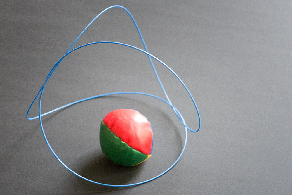
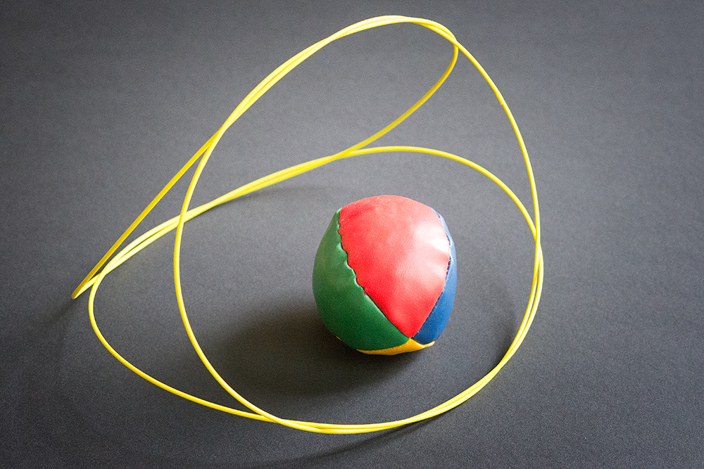
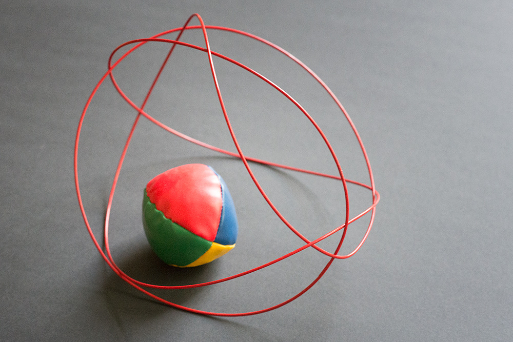
Figure 1.1: Springy knots: figure-eight knot, mathematician’s loop, and Chinese button knot. Wire models manufactured by why knots, Box 635, Aptos, CA 95003, in 1980; coloured photographs by B. Bollwerk, Aachen.

Mathematically, the classification of elastic knots is a fascinating problem, and our aim is to justify the behaviour of the trefoil and of more general torus knots by means of the simplest possible model in elasticity. Ignoring all effects of extension and shear the wire is represented by a sufficiently smooth closed curve $\gamma:\mathbb{R}/\mathbb{Z}\to\mathbb{R}^{3}$ of unit length and parametrized by arclength (referred to as unit loop). We follow Bernoulli’s approach to consider the bending energy

$$E_{\mathrm{bend}}(\gamma):=\int_{\gamma}\varkappa^{2}\,\mathrm{d}s$$ (1.1)

as the only intrinsic elastic energy—neglecting any additional torsional effects, and we also exclude external forces and friction that might be present in Langer’s toy models. Here, $\varkappa=|\gamma^{\prime\prime}|$ is the classic local curvature of the curve. To respect a given knot class when minimizing the bending energy we have to preclude self-crossings. In principle we could add any self-repulsive knot energy for that matter, imposing infinite energy barriers between different knot classes; see, e.g., the recent surveys [5, 6, 33, 34] on such energies and their impact on geometric knot theory. But a solid (albeit thin) wire motivates a steric constraint in form of a fixed (small) thickness of all curves in competition. This, and the geometric rigidity it imposes on the curves lead us to adding a small amount of ropelength $\mathcal{R}$ to form the total energy

$$E_{\vartheta}:=E_{\mathrm{bend}}+\vartheta\mathcal{R},\qquad\vartheta>0,$$ (1.2)

to be minimized within a prescribed tame knot class $\mathcal{K}$, that is, on the class $\mathscr{C}(\mathcal{K})$ of all unit loops representing $\mathcal{K}$. As ropelength is defined as the quotient of length and thickness it boils down for unit loops to $\mathcal{R}(\gamma)=1/\triangle[\gamma]$. Following Gonzalez and Maddocks [16] the thickness $\triangle[\cdot]$ may be expressed as

$$\triangle[\gamma]:=\inf_{u,v,w\in\mathbb{R}/\mathbb{Z}\atop u\not=v\not=w\not=u}R(\gamma(u),\gamma(v),\gamma(w)),$$ (1.3)

where $R(x,y,z)$ denotes the unique radius of the (possibly degenerate) circle passing through $x,y,z\in\mathbb{R}^{3}.$

By means of the direct method in the calculus of variations we show that in every given (tame) knot class $\mathcal{K}$ and for every $\vartheta>0$ there is indeed a unit loop $\gamma_{\vartheta}\in\mathscr{C}(\mathcal{K})$ minimizing the total energy $E_{\vartheta}$ within $\mathcal{K}$; see Theorem 2.1 in Section 2.

To understand the behaviour of very thin springy knots we investigate the limit $\vartheta\to 0$. More precisely, we consider arbitrary sequences $(\gamma_{\vartheta})_{\vartheta}$ of minimizers in a fixed knot class $\mathcal{K}$ and look at their possible limit curves $\gamma_{0}$ as $\vartheta\to 0$. We call any such limit curve an elastic knot for $\mathcal{K}$. None of these elastic knots is embedded (as we would expect in view of the self-contact present in the wire models in Figure 1.1)—unless $\mathcal{K}$ is the unknot, in which case $\gamma_{0}$ is the once-covered circle; see Proposition 3.1. However, it turns out that each elastic knot $\gamma_{0}$ lies in the $C^{1}$-closure of unit loops representing ${\mathcal{K}}$, and non-trivial elastic knots can be shown to have strictly smaller bending energy $E_{\mathrm{bend}}$ than any unit loop in $\mathscr{C}(\mathcal{K})$ (Theorem 2.2). This minimizing property of elastic knots is particularly interesting for those non-trivial knot classes $\mathcal{K}$ permitting representatives with bending energy arbitrarily close to the smallest possible lower bound $(4\pi)^{2}$ (due to Fáry’s and Milnor’s lower bound $4\pi$ on total curvature [13, 24]): We can show that for those knot classes the only possible shape of any elastic knot is that of the twice-covered circle. This naturally leads to the question:

For which knot classes $\mathcal{K}$ do we have $\inf_{\mathscr{C}(\mathcal{K})}E_{\mathrm{bend}}=(4\pi)^{2}$?

We are going to show that this is true exactly for the class $\mathcal{T}(2,b)$ of $(2,b)$-torus knots for any odd integer $b$ with $|b|\geq 3.$ Any other non-trivial knot class has a strictly larger infimum of bending energy. These facts and several other characterizations of $\mathcal{T}(2,b)$ are contained in our Main Theorem 6.3, from which we can extract the following complete description of elastic $(2,b)$-torus knots (including the trefoil):

Theorem 1.1 (Elastic $(2,b)$-torus knots).

For any odd integer $\left|b\right|\geq 3$ the unique elastic $(2,b)$-torus knot is the twice-covered circle.

This result confirms our mechanical and numerical experiments (see Figure 1.3 on the left and Figure 1.2), as well as the heuristics and the Metropolis Monte Carlo simulations of Gallotti and Pierre-Louis [15], and the numerical gradient-descent results by Avvakumov and Sossinsky, see [2] and references therein.

Our results especially affect knot classes with bridge number two (see below for the precise definition) which in the majority of cases appear in applications, e.g., DNA knots, see Sumners [35, p. 338]. The Main Theorem 6.3, however, implies also that for knots different from the $(2,b)$-torus knots, the respective elastic knot is definitely not the twice-covered circle. Similar shapes as in Figure 1.2 have been obtained numerically by Buck and Rawdon [8] for a related but different variational problem: they minimize ropelength with a prescribed curvature bound (using a variant of the Metropolis Monte Carlo procedure), see [8, Fig. 8].

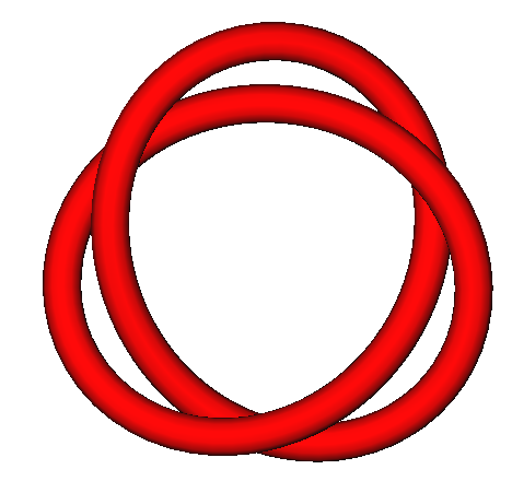
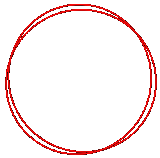
$\vartheta=0.1$	$\vartheta=0.001$

Figure 1.2: Minimizers of the total energy $E_{\vartheta}$ in the class of trefoils approaching the twice covered circle as $\vartheta$ tends to zero. For numerical reasons the ropelength $\mathcal{R}$ was substituted by a repulsive potential, the Möbius energy introduced by O’Hara [25].

The idea of studying $\gamma_{0}$ as a limit configuration of minimizers of the mildly penalized bending energy goes back to earlier work of the third author [36], only that there ropelength in (1.2) is replaced by a self-repulsive potential, like the Möbius energy introduced by O’Hara [25]. By means of a Li-Yau-type inequality for general loops [36, Theorem 4.4] it was shown there that for elastic $(2,b)$-torus knots, the maximal multiplicity of double points is three [36, p. 51]. Theorem 1.1 clearly shows that this multiplicity bound is not sharp: the twice-covered circle has infinitely many double points all of which have multiplicity two. Lin and Schwetlick [21] consider the gradient flow of the elastic energy plus the Möbius energy scaled by a certain parameter. However, there is no analysis of the equilibrium shapes, and they do not consider the limit case of sending the prefactor of the Möbius term to zero.

Directly analyzing the shape or even only the regularity of the $E_{\vartheta}$-minimizers $\gamma_{\vartheta}$ for positive $\vartheta$ without going to the limit $\vartheta\to 0$ seems much harder because of a priorily unknown (and possibly complicated) regions of self-contact that are determined by the minimizers $\gamma_{\vartheta}$ themselves. Necessary conditions were derived by a Clarke-gradient approach in [30] for nonlinearly elastic rods, and for an alternative elastic self-obstacle formulation regularity results were established in [37] depending on the geometry of contact. If one replaces ropelength in (1.2) by a self-repulsive potential like in [36] one can prove $C^{\infty}$-smoothness of $\gamma_{\vartheta}$ with the deep analytical methods developed by He [18], and the second author in various cooperations [27, 28, 4, 7]. But the corresponding Euler-Lagrange equations for $E_{\vartheta}$ involving complicated non-local terms do not seem to give immediate access to determining the shape of $\gamma_{\vartheta}.$ Notice that directly minimizing the bending energy $E_{\mathrm{bend}}$ in the $C^{1}$-closure of $\mathscr{C}(\mathcal{K})$ generally leads to a much larger number of minimizers of which the majority seems to correspond to quite unstable configurations in physical experiments. Our approach of penalizing the bending energy by $\vartheta$ times ropelength and approximating zero thickness by letting $\vartheta\to 0$ may be viewed as selecting those $E_{\mathrm{bend}}$-minimizers that correspond to physically reasonable springy knots with sufficiently small thickness.

Recall that our simple model neglects any effects of torsion. Twisting the wire in the experiments before closing it at the hinge (without releasing the twist) leads to completely different stable configurations; see Figure 1.3 on the right. So, in that case a more general Lagrangian taking into account also these torsional effects would need to be considered, and the question of classifying elastic knots with torsion is wide open.

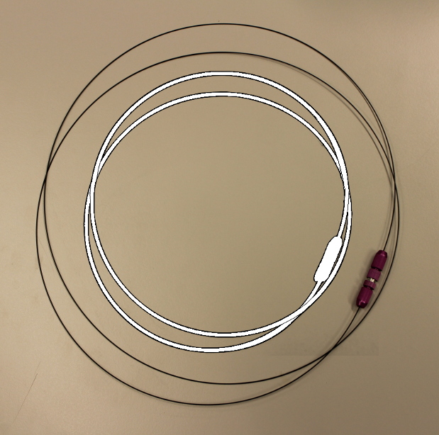
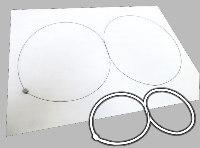
Figure 1.3: Mechanical experiments. Left: The springy trefoil knot is close to the twice-covered circle. Right: Adding a twist leads to a stable flat trefoil configuration close to a planar figure-eight. Wire models by courtesy of John H. Maddocks, Lausanne.

This is our strategy:

In Section 2 we establish first the existence of minimizers $\gamma_{\vartheta}$ of the total energy $E_{\vartheta}$ for each positive $\vartheta$ (Theorem 2.1). Then we pass to the limit $\vartheta\to 0$ to obtain a limit configuration $\gamma_{0}$ in the $C^{1}$-closure of $\mathscr{C}(\mathcal{K})$ whose bending energy $E_{\mathrm{bend}}(\gamma_{0})$ serves as a lower bound on $E_{\mathrm{bend}}$ in $\mathscr{C}(\mathcal{K})$; see Theorem 2.2. By means of the classic uniqueness result of Langer and Singer [20] on stable elasticae in $\mathbb{R}^{3}$ we identify in Proposition 3.1 the round circle as the unique elastic unknot. Elastic knots for knot classes with $(4\pi)^{2}$ as sharp lower bound on the bending energy turn out to have constant curvature $4\pi$; see Proposition 3.2. By a Schur-type result (Proposition 3.3) we can use this curvature information to establish a preliminary classification of such elastic knots as tangential pairs of circles, i.e., as pairs of round circles each with radius $1/(4\pi)$ with (at least) one point of tangential intersection; see Figure 3.1 and Corollary 3.4. The key here to proving constant curvature is an extension of the classic Fáry–Milnor theorem on total curvature to the $C^{1}$-closure of $\mathscr{C}(\mathcal{K})$; see Theorem A.1 in the Appendix. Our argument for that extension crucially relies on Denne’s result on the existence of alternating quadrisecants [11]. The fact that the elastic knot $\gamma_{0}$ for $\mathcal{K}$ is a tangential pair of circles implies by means of Proposition 4.6 that $\mathcal{K}$ is actually the class $\mathcal{T}(2,b)$ for odd $b$ with $|b|\geq 3$.

In order to extract the doubly-covered circle from the one-parameter family of tangential pairs of circles as the only possible elastic knot for $\mathcal{T}(2,b)$ we use in Section 5 explicit $(2,b)$-torus knots as suitable comparison curves. Estimating their bending energies and thickness values allows us to establish improved growth estimates for the total energy and ropelength of the $E_{\vartheta}$-minimizers $\gamma_{\vartheta}$; see Proposition 5.4. In his seminal article [24] Milnor derived the lower bound for the total curvature by studying the crookedness of a curve and relating it to the total curvature. For some regular curve $\gamma:\mathbb{R}/\mathbb{Z}\to\mathbb{R}^{3}$ its crookedness is the infimum over all $\nu\in\mathbb{S}^{2}$ of

$$\mu(\gamma,\nu):=\#\left\{t_{0}\in\mathbb{R}/\mathbb{Z}\,\middle|\,t_{0}\textnormal{ is a local maximizer of }t\mapsto\left\langle\gamma(t),\nu\right\rangle_{\mathbb{R}^{3}}\right\}.$$ (1.4)

For any curve $\gamma$ close to a tangential pair of circles that is not the doubly covered circle we can show in Lemma 6.2 that the set of directions $\nu\in\mathbb{S}^{2}$ for which $\mu(\gamma,\nu)\geq 3$ is bounded in measure from below by some multiple of thickness $\triangle[\gamma]$. Assuming finally that $\gamma_{\vartheta}$ converges for $\vartheta\to 0$ to such a limiting tangential pair of circles different from the doubly covered circle we use this crookedness estimate to obtain a contradiction against the total energy growth rate proved in Proposition 5.4. Therefore, the only possible limit configuration $\gamma_{0}$, i.e., elastic knot in the class of $(2,b)$-torus knots, is the doubly covered circle.

As pointed out above, the heart of our argument consists of two bounds on the bending energy, the lower one, $(4\pi)^{2}$, imposed by the Fáry–Milnor inequality, the upper one given by comparison curves. The latter ones are constructed by considering a suitable $(2,b)$-torus knot lying on a (standard) torus and then shrinking the width of the torus to zero, such that the bending energy of the torus knot tends to the lower bound $(4\pi)^{2}$. This indicates that a more general result should be valid if these bounds can be extended to other knot classes.

Milnor [24] proved that the lower bound on the total curvature is in fact $2\pi\operatorname{bri}\mathcal{K}$ where $\operatorname{bri}\mathcal{K}$ denotes the bridge index, i.e., the minimum of crookedness over the knot class $\mathcal{K}$. So we should ask which knot classes $\mathcal{K}$ can be represented by a curve made of a number of strands, say $a$ strands, passing inside a (full) torus, virtually in the direction of its central core. The minimum value for $a$ with respect to the knot class $\mathcal{K}$ is referred to as braid index, $\operatorname{bra}\mathcal{K}$. Thus we are led to believing that the following assertion holds true which has already been stated by Gallotti and Pierre-Louis [15].

Conjecture 1.2 (Circular elastic knots).

The $a$-times covered circle is the (unique) elastic knot for the (tame) knot class $\mathcal{K}$ if $\operatorname{bra}\mathcal{K}=\operatorname{bri}\mathcal{K}=a$. $\Diamond$

The shape of elastic knots for more general knot classes is one of the topics of ongoing research. Here we only mention a conjecture that has personally been communicated to the third author by Urs Lang in 1997.

Conjecture 1.3 (Spherical elastic knots).

Any elastic prime knot is a spherical or planar curve. $\Diamond$

Our numerical experiments (see Figures 1.2 and 1.4) as well as the simulations performed by Gallotti and Pierre-Louis [15, Figs. 6 & 7] seem to support this conjecture.

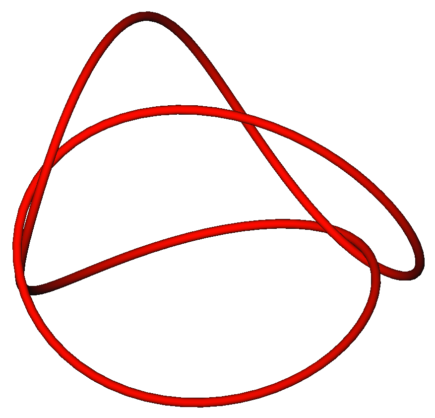
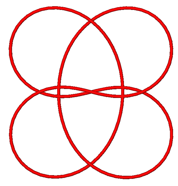
Figure 1.4: Simulated annealing experiments for other knot classes. Left: The figure-eight knot ($4_{1}$) (resembling the blue springy figure-eight in Figure 1.1) seems to lie on a sphere. Right: A planar Chinese button knot ($9_{40}$) (in contrast to the spherical red springy wire in Figure 1.1 indicating that tying a more complex wire knot may impose some amount of physical torsion in addition to pure bending).

Acknowledgements.

The second author was partially supported by DFG Transregional Collaborative Research Centre SFB TR 71. We gratefully acknowledge stimulating discussions with Elizabeth Denne, Sebastian Scholtes, and John Sullivan. We would like to thank Thomas El Khatib for bringing reference [15] to our attention.

2 Existence of elastic knots

To ease notation we shall simply identify the intrinsic distance on $\mathbb{R}/\mathbb{Z}$ with $|x-y|$, that is,

$$|x-y|\equiv|x-y|_{\mathbb{R}/\mathbb{Z}}:=\min\{|x-y|,1-|x-y|\}.$$

For any knot class $\mathcal{K}$ we define the class $\mathscr{C}(\mathcal{K})$ of unit loops representing $\mathcal{K}$ as

$$\mathscr{C}(\mathcal{K}):=\{\gamma\in H^{2}(\mathbb{R}/\mathbb{Z},\mathbb{R}^{3}):\gamma(0)=0,|\gamma^{\prime}|\equiv 1\,{\textnormal{on\,\,}}\,\mathbb{R}/\mathbb{Z},\textnormal{\,$\gamma$ is of knot type $\mathcal{K}$}\},$$

where $H^{2}(\mathbb{R}/\mathbb{Z},\mathbb{R}^{3})$ denotes the class of $1$-periodic Sobolev functions whose second weak derivatives are square-integrable. The bending energy (1.1) on the space of curves $\gamma\in H^{2}(\mathbb{R}/L\mathbb{Z},\mathbb{R}^{3})$, $L>0$, reads as

$$E_{\mathrm{bend}}(\gamma)=\int_{\gamma}\varkappa^{2}\,\mathrm{d}s=\int_{\mathbb{R}/L\mathbb{Z}}\varkappa^{2}\left|\gamma^{\prime}\right|\,\mathrm{d}t=\int_{0}^{L}\frac{\left|\gamma^{\prime\prime}\wedge\gamma^{\prime}\right|^{2}}{\left|\gamma^{\prime}\right|^{5}}\,\mathrm{d}t,$$ (2.1)

which reduces to the squared $L^{2}$-norm $\|\gamma^{\prime\prime}\|^{2}_{L^{2}}$ of the (weak) second derivative $\gamma^{\prime\prime}$ if $\gamma$ is parametrized by arclength. The ropelength functional defined as the quotient of length and thickness simplifies on $\mathscr{C}(\mathcal{K})$ to

$$\mathcal{R}(\gamma)=\frac{1}{\triangle[\gamma]},$$ (2.2)

where thickness $\triangle[\gamma]$ can be expressed as in (1.3). For $\vartheta>0$ we want to minimize the total energy $E_{\vartheta}$ as given in (1.2) on the class $\mathscr{C}(\mathcal{K})$ of unit loops representing $\mathcal{K}$. Note that, in contrast to the bending energy, a unit loop in $\mathscr{C}(\mathcal{K})$ has finite total energy $E_{\vartheta}$ if and only if it belongs to $C^{1,1}$, see [17, Lemma 2] and [31, Theorem 1 (iii)].

Theorem 2.1 (Minimizing the total energy).

For any fixed tame knot class $\mathcal{K}$ and for each $\vartheta>0$ there exists a unit loop $\gamma_{\vartheta}\in\mathscr{C}(\mathcal{K})$ such that

$$E_{\vartheta}(\gamma_{\vartheta})=\inf_{\mathscr{C}(\mathcal{K})}E_{\vartheta}(\cdot).$$ (2.3)

Proof 1.

The total energy is obviously nonnegative, and $\mathscr{C}(\mathcal{K})$ is not empty since one may scale any smooth representative of $\mathcal{K}$ (which exists due to tameness) down to length one and reparametrize to arclength, so that the infimum in (2.3) is finite. Taking a minimal sequence $(\gamma_{k})_{k}\subset\mathscr{C}(\mathcal{K})$ with $E_{\vartheta}(\gamma_{k})\to\inf_{\mathscr{C}(\mathcal{K})}E_{\vartheta}$ as $k\to\infty$ we get the uniform bound

$$\|\gamma_{k}^{\prime\prime}\|_{L^{2}}^{2}=E_{\mathrm{bend}}(\gamma_{k})\leq E_{\vartheta}(\gamma_{k})\leq 1+\inf_{\mathscr{C}(\mathcal{K})}E_{\vartheta}<\infty\quad{\textnormal{for all\,\,}}k\gg 1,$$

so that with $\gamma_{k}(0)=0$ and $|\gamma_{k}^{\prime}|\equiv 1$ for all $k\in\mathbb{N}$ we have a uniform bound on the full $H^{2}$-norm of the $\gamma_{k}$ independent of $k$ for $k$ sufficiently large. Since $H^{2}(\mathbb{R}/\mathbb{Z},\mathbb{R}^{3})$ as a Hilbert space is reflexive and $H^{2}(\mathbb{R}/\mathbb{Z},\mathbb{R}^{3})$ is compactly embedded in $C^{1}(\mathbb{R}/\mathbb{Z},\mathbb{R}^{3})$ this implies the existence of some $\gamma_{\vartheta}\in H^{2}(\mathbb{R}/\mathbb{Z},\mathbb{R}^{3})$ and a subsequence $(\gamma_{k_{i}})_{i}\subset(\gamma_{k})_{k}$ converging weakly in $H^{2}$ and strongly in $C^{1}$ to $\gamma_{\vartheta}$ as $i\to\infty.$ Thus we obtain $\gamma_{\vartheta}(0)=0$ and $|\gamma_{\vartheta}^{\prime}|\equiv 1$ on $\mathbb{R}/\mathbb{Z}.$ Since thickness is upper semicontinuous [17, Lemma 4] and the bending energy lower semicontinuous with respect to this type of convergence we arrive at

$$E_{\vartheta}(\gamma_{\vartheta})\leq\liminf_{i\to\infty}E_{\vartheta}(\gamma_{k_{i}})=\inf_{\mathscr{C}(\mathcal{K})}E_{\vartheta}(\cdot)<\infty.$$ (2.4)

In particular by definition of $E_{\vartheta}$, one has $\mathcal{R}(\gamma_{\vartheta})<\infty$ or $\triangle[\gamma_{\vartheta}]>0$, which implies by [17, Lemma 1] that $\gamma_{\vartheta}$ is embedded. As all closed curves in a $C^{1}$-neighbourhood of a given embedded curve are isotopic, as shown by Diao, Ernst, and Janse van Rensburg [12, Lemma 3.2], see also [3, 26], we find that $\gamma_{\vartheta}$ is of knot type $\mathcal{K}$; hence $\gamma_{\vartheta}\in\mathscr{C}(\mathcal{K}).$ This gives $\inf_{\mathscr{C}(\mathcal{K})}E_{\vartheta}(\cdot)\leq E_{\vartheta}(\gamma_{\vartheta})$, which in combination with (2.4) concludes the proof. $\Box$

Since finite ropelength, i.e., positive thickness, implies $C^{1,1}$-regularity we know that $\gamma_{\vartheta}\in C^{1,1}(\mathbb{R}/\mathbb{Z},\mathbb{R}^{3})$. However, we are not going to exploit this improved regularity, since we investigate the limit $\vartheta\to 0$ and the corresponding limit configurations, the elastic knots $\gamma_{0}$ for the given knot class $\mathcal{K}$.

Theorem 2.2 (Existence of elastic knots).

Let $\mathcal{K}$ be any fixed tame knot class, $\vartheta_{i}\to 0$ and $(\gamma_{\vartheta_{i}})_{i}\subset\mathscr{C}(\mathcal{K})$, such that $E_{\vartheta_{i}}(\gamma_{\vartheta_{i}})=\inf_{\mathscr{C}(\mathcal{K})}E_{\vartheta_{i}}(\cdot)$ for each $i\in\mathbb{N}.$ Then there exists $\gamma_{0}\in H^{2}(\mathbb{R}/\mathbb{Z},\mathbb{R}^{3})$ and a subsequence $(\gamma_{\vartheta_{i_{k}}})_{k}\subset(\gamma_{\vartheta_{i}})_{i}$ such that the $\gamma_{\vartheta_{i_{k}}}$ converge weakly in $H^{2}$ and strongly in $C^{1}$ to $\gamma_{0}$ as $k\to\infty$. Moreover,

$$E_{\mathrm{bend}}(\gamma_{0})\leq E_{\mathrm{bend}}(\beta)\quad{\textnormal{for all\,\,}}\beta\in\mathscr{C}(\mathcal{K}).$$ (2.5)

The estimate (2.5) is strict unless $\mathcal{K}$ is the unknot class.

Definition 2.3 (Elastic knots).

Any curve $\gamma_{0}$ as in Theorem 2.2 is called an elastic knot for $\mathcal{K}$.

Proof 2 (Theorem 2.2).

For any $\beta\in\mathscr{C}(\mathcal{K})$ and any $\vartheta>0$ we can estimate

$$E_{\mathrm{bend}}(\gamma_{\vartheta})\leq E_{\vartheta}(\gamma_{\vartheta})\leq E_{\vartheta}(\beta),$$ (2.6)

where $\gamma_{\vartheta}\in\mathscr{C}(\mathcal{K})$ is a global minimizer of $E_{\vartheta}$ within $\mathscr{C}(\mathcal{K})$ whose existence is guaranteed by Theorem 2.1. Now we restrict to $\beta\in\mathscr{C}(\mathcal{K})\cap C^{1,1}(\mathbb{R}/\mathbb{Z},\mathbb{R}^{3})$, which implies by means of [31, Theorem 1 (iii)] that the right-hand side of (2.6) is finite. Now the right-hand side tends to $E_{\mathrm{bend}}(\beta)<\infty$ as $\vartheta\to 0$ and we find a constant $C$ independent of $\vartheta$ such that

$$\|\gamma_{\vartheta}\|_{H^{2}}\leq C\quad{\textnormal{for all\,\,}}\vartheta\in(0,1).$$ (2.7)

In particular, this uniform estimate holds for the $\gamma_{\vartheta_{i}}\in\mathscr{C}(\mathcal{K})$ so that there is $\gamma_{0}\in H^{2}(\mathbb{R}/\mathbb{Z},\mathbb{R}^{3})$ and a subsequence $(\gamma_{\vartheta_{i_{k}}})_{k}\subset(\gamma_{\vartheta_{i}})_{i}$ with $\gamma_{\vartheta_{i_{k}}}\rightharpoonup\gamma_{0}$ in $H^{2}$ and $\gamma_{\vartheta_{i_{k}}}\to\gamma_{0}$ in $C^{1}$ as $k\to\infty.$ The bending energy $E_{\mathrm{bend}}$ is lower semicontinuous with respect to weak convergence in $H^{2}$ which implies

$$E_{\mathrm{bend}}(\gamma_{0})\leq\liminf_{k\to\infty}E_{\mathrm{bend}}(\gamma_{\vartheta_{i_{k}}})\overset{\eqref{bending-estimate}}{\leq}\liminf_{k\to\infty}E_{\vartheta_{i_{k}}}(\beta)=E_{\mathrm{bend}}(\beta).$$

Thus we have established (2.5) for any $\beta\in\mathscr{C}(\mathcal{K})\cap C^{1,1}(\mathbb{R}/\mathbb{Z},\mathbb{R}^{3})$. In order to extend it to the full domain, we approximate an arbitrary $\beta\in\mathscr{C}(\mathcal{K})$ by a sequence of functions $\left({\beta}_{k}\right)_{k\in\mathbb{N}}\subset C^{\infty}(\mathbb{R}/\mathbb{Z},\mathbb{R}^{3})$ with respect to the $H^{2}$-norm. As $H^{2}$ embeds into $C^{1,1/2}$, the tangent vectors $\beta_{k}^{\prime}$ uniformly converge to $\beta^{\prime}$, so $\left|\beta_{k}^{\prime}\right|\geq c>0$ for all $k\gg 1$.

Furthermore, the $\beta_{k}$ are injective since for $\beta$ there are positive constants $c$ and $\varepsilon$ depending only on $\beta$ such that

$$|\beta(s)-\beta(t)|\geq c|s-t|_{\mathbb{R}/\mathbb{Z}}\quad{\textnormal{for all\,\,}}|s-t|_{\mathbb{R}/\mathbb{Z}}<\varepsilon,$$

because $|\beta^{\prime}|\equiv 1$, and in consequence, there is another constant $\delta=\delta(\beta)\in(0,c\varepsilon]$ such that

$$|\beta(s)-\beta(t)|\geq\delta\quad{\textnormal{for all\,\,}}|s-t|_{\mathbb{R}/\mathbb{Z}}\geq\varepsilon,$$

for $\beta$ is injective. Consequently, for given distinct parameters $s,t\in[0,1)$ we can estimate

$$|\beta_{k}(s)-\beta_{k}(t)|\geq|\beta(s)-\beta(t)|-2\|\beta_{k}^{\prime}-\beta^{\prime}\|_{L^{\infty}}|s-t|_{\mathbb{R}/\mathbb{Z}},$$

which is positive for $k\gg 1$ independent of the intrinsic distance $|s-t|_{\mathbb{R}/\mathbb{Z}}$. In addition, the $\beta_{k}$ represent the same knot class $\mathcal{K}$ as $\beta$ does for $k\gg 1$, since isotopy is stable under $C^{1}$-convergence [12, 3, 26]. According to [28, Thm. A.1] the sequence $\left({\tilde{\beta}}_{k}\right)_{k\in\mathbb{N}}$ of smooth curves, where $\tilde{\beta}_{k}$ is obtained from $\beta_{k}$ (after omitting finitely many $\beta_{k}$) by rescaling to unit length and then reparametrizing to arc-length, converges to $\tilde{\beta}=\beta$ with respect to the $H^{2}$-norm, and, of course, $\tilde{\beta}_{k}\in\mathscr{C}(\mathcal{K})$ for all $k$. We conclude

$$E_{\mathrm{bend}}(\gamma_{0})\leq E_{\mathrm{bend}}(\tilde{\beta}_{k})=\left\|\tilde{\beta}_{k}^{\prime\prime}\right\|_{L^{{2}}}^{2}\to\left\|\beta^{\prime\prime}\right\|_{L^{{2}}}^{2}=E_{\mathrm{bend}}(\beta).$$

Assume now $E_{\mathrm{bend}}(\gamma_{0})=E_{\mathrm{bend}}(\beta)$ for some $\beta\in\mathscr{C}(\mathcal{K})$ where $\mathcal{K}$ is non-trivial. In this case, $\beta$ would be a local minimizer, and therefore a stable closed elastica as there are no restrictions for variations. According to the result of J. Langer and D. A. Singer [20], $\beta$ turns out to be the round circle, hence $\mathcal{K}$ is the unknot, contradiction. $\Box$

3 The elastic unknot and tangential pairs of circles

The springy knotted wires strongly suggest that we should expect that the elastic knots generally exhibit self-intersections, and this is indeed the case unless the knot class is trivial. In fact, the elastic unknot is the round circle of length one.

Proposition 3.1 (Non-trivial elastic knots are not embedded).

The round circle of length one is the unique elastic unknot. If there exists an embedded elastic knot $\gamma_{0}$ for a given knot class $\mathcal{K}$ then $\mathcal{K}$ is the unknot (so that $\gamma_{0}$ is the round circle of length one). In particular, if $\mathcal{K}$ is a non-trivial knot class, every elastic knot for $\mathcal{K}$ must have double points.

Proof 3.

The round circle of length one uniquely minimizes $E_{\mathrm{bend}}$ and $\mathcal{R}$ simultaneously in the class of all arclength parametrized curves in $H^{2}(\mathbb{R}/\mathbb{Z},\mathbb{R}^{3}).$ For the bending energy $E_{\mathrm{bend}}$ this is true since the round once-covered circle is the only stable closed elastica in $\mathbb{R}^{3}$ according to the work of J. Langer and D. A. Singer [20], and for ropelength this follows, e.g., from the more general uniqueness result in [32, Lemma 7] for the functionals

$$\mathcal{U}_{p}(\gamma):=\left(\int_{\gamma}\sup_{v,w\in\mathbb{R}/\mathbb{Z}\atop u\not=v\not=w\not=u}R^{-p}(\gamma(u),\gamma(v),\gamma(w))\,\mathrm{d}u\right)^{1/p},\quad p\geq 1.$$

For closed rectifiable curves $\gamma$ different from the round circle with $\mathcal{R}(\gamma)<\infty$ one has indeed

$$2\pi=\mathcal{R}(\textnormal{circle})=\mathcal{U}_{p}(\textnormal{circle})\overset{\text{\cite[cite]{[\@@bibref{}{SvdM07}{}{}, Lem.~{}7]}}}{<}\mathcal{U}_{p}(\gamma)\leq\mathcal{R}(\gamma).$$

Hence the round circle uniquely minimizes also the total energy $E_{\vartheta}$ for each $\vartheta>0$ in $\mathscr{C}(\mathcal{K})$ when $\mathcal{K}$ is the unknot. Thus any elastic unknot as the $C^{1}$-limit of $E_{\vartheta_{i}}$-minimizers as $\vartheta_{i}\to 0$ is also the round circle of length one.

If $\gamma_{0}$ is embedded then according to the stability of isotopy classes under $C^{1}$-perturbations (see [12, 3, 26]) we find $\gamma_{0}\in\mathscr{C}(\mathcal{K})$ since $\gamma_{0}$ was obtained as the weak $H^{2}$-limit of $E_{\vartheta_{i}}$-minimizers $\gamma_{\vartheta_{i}}\in\mathscr{C}(\mathcal{K}).$ Thus, by (2.5), the curve $\gamma_{0}$ is a local minimizer of $E_{\mathrm{bend}}$ in $\mathscr{C}(\mathcal{K})$, and therefore it is a stable elastica. Thus, again by the stability result of Langer and Singer, $\gamma_{0}$ is the round circle of length one. Consequently, $\mathcal{K}$ is the unknot, which proves the proposition. $\Box$

In the appendix we extend the Fáry–Milnor theorem to the $C^{1}$-closure of $\mathscr{C}(\mathcal{K})$, where $\mathcal{K}$ is a non-trivial knot class; see Theorem A.1. This allows us in a first step to show that elastic knots for $\mathcal{K}$ have constant curvature if one can get arbitrarily close with the bending energy in $\mathscr{C}(\mathcal{K})$ to the natural lower bound $(4\pi)^{2}$ induced by Fáry and Milnor.

Proposition 3.2 (Elastic knots of constant curvature).

For any knot class $\mathcal{K}$ with

$$\inf_{\mathscr{C}(\mathcal{K})}E_{\mathrm{bend}}=(4\pi)^{2}$$ (3.1)

one has $\varkappa_{\gamma_{0}}=4\pi$ a.e. on $\mathbb{R}/\mathbb{Z}$ for each elastic knot $\gamma_{0}$ for $\mathcal{K}$. In particular, $\gamma_{0}\in C^{1,1}(\mathbb{R}/\mathbb{Z},\mathbb{R}^{3}).$

Proof 4.

According to our generalized Fáry–Milnor Theorem, Theorem A.1 in the Appendix applied to $\gamma_{0}\in\overline{\mathscr{C}(\mathcal{K})}^{C^{1}}$, we estimate by means of Hölder’s inequality

$$(4\pi)^{2}\overset{\eqref{eq:fm}}{\leq}\left(\int_{\gamma_{0}}\varkappa_{\gamma_{0}}\right)^{2}\leq E_{\mathrm{bend}}(\gamma_{0})\stackrel{{\scriptstyle\eqref{bendminimizing}}}{{\leq}}\inf_{\mathscr{C}(\mathcal{K})}E_{\mathrm{bend}}\stackrel{{\scriptstyle\eqref{infimaequal}}}{{=}}(4\pi)^{2},$$

hence equality everywhere. In particular, equality in Hölder’s inequality implies a constant integrand, which we calculate to be $\varkappa_{\gamma_{0}}=4\pi$ a.e. on $\mathbb{R}/\mathbb{Z}$. $\Box$

Of course, there are many closed curves of constant curvature, see e.g. Fenchel [14], even in every knot class, see McAtee [23]. Closed spaces curves of constant curvature may, e.g., be constructed by joining suitable arcs of helices, see Koch and Engelhardt [19] for an explicit construction and examples. But in order to identify the possible shape of elastic knots for knot classes that satisfy assumption (3.1) recall that any minimizer in a non-trivial knot class has at least one double point; see Proposition 3.1. In addition, the length is fixed to one, so that we can reduce the possible shapes of elastic knots considerably by means of a Schur-type argument that connects length and constant curvature; see the following Proposition 3.3. This will in particular lead to the proof of the classification result, Theorem 6.3.

Proposition 3.3 (Shortest arc of constant curvature).

Let $\gamma\in H^{2}([0,L],\mathbb{R}^{3})$, $L>0$, be parametrized by arc-length with constant curvature $\varkappa=\left|\gamma^{\prime\prime}\right|=4\pi$ a.e. and coinciding endpoints $\gamma(0)=\gamma(L)$. Then $L\geq\frac{1}{2}$ with equality if and only if $\gamma$ is a circle with radius $\frac{1}{4\pi}$.

Before proving this rigidity result let us note an immediate consequence.

Corollary 3.4 (Tangential pairs of circles).

Every closed arclength parametrized curve $\gamma\in H^{2}(\mathbb{R}/\mathbb{Z},\mathbb{R}^{3})$ with at least one double point and with constant curvature $\varkappa_{\gamma}=|\gamma^{\prime\prime}|=4\pi$ a.e. on $\mathbb{R}/\mathbb{Z}$, is a tangential pair of circles. That is, $\gamma$ belongs, up to isometry and parametrization, to the one-parameter family of tangentially intersecting circles

$$\operatorname{tpc}_{\varphi}:t\mapsto\tfrac{1}{4\pi}\begin{cases}\mathbf{e}_{1}(1-\cos(4\pi t))-\mathbf{e}_{2}\sin(4\pi t),&t\in[0,\tfrac{1}{2}],\\ (\mathbf{e}_{1}\cos\varphi+\mathbf{e}_{3}\sin\varphi)(1-\cos(4\pi t))-\mathbf{e}_{2}\sin(4\pi t),&t\in[\tfrac{1}{2},1],\end{cases}$$ (3.2)

where $\varphi\in[0,\pi]$. Here $\mathbf{e}_{k}$ denotes the $k$-th unit vector in $\mathbb{R}^{3}$, $k=1,2,3$.

Note that $\operatorname{tpc}_{0}$ is a doubly covered circle and $\operatorname{tpc}_{\pi}$ a tangentially intersecting planar figure eight, both located in the plane spanned by $\mathbf{e}_{1}$ and $\mathbf{e}_{2}$. For intermediate values $\varphi\in(0,\pi)$ one obtains a configuration as shown in Figure 3.1.

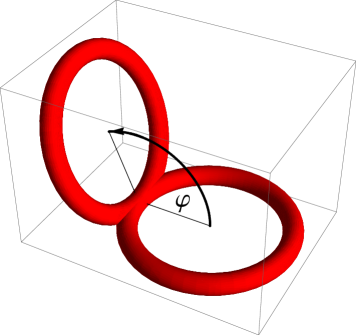
Figure 3.1: Plot of $\operatorname{tpc}_{\varphi}$ for $\varphi={\nicefrac{{5\pi}}{{8}}}$

Proof 5 (Corollary 3.4).

Applying Proposition 3.3 we find that the length of any arc starting from a double point amounts to at least $\tfrac{1}{2}$. As $\mathscr{L}(\gamma)=1$ we have precisely two arcs of length $\tfrac{1}{2}$ between each double point which again by Proposition 3.3 implies that both these connecting arcs are circles of radius $\tfrac{1}{4\pi}$. They have to meet tangentially due to the embedding $H^{2}\hookrightarrow C^{1,1/2}$. Thus $\gamma=\operatorname{tpc}_{\varphi}$ for some $\varphi\in[0,\pi]$. $\Box$

Proof 6 (Proposition 3.3).

Obviously, the statement is equivalent to minimizing $L>0$ over $f=\gamma^{\prime}\in H^{1}([0,L],\mathbb{S}^{2})$ with $\left|f^{\prime}\right|=4\pi$ a.e. and $\int_{0}^{L}f=0$. As $f\not\equiv 0$ there is some $T\in(0,L)$ maximizing $t\mapsto\left|\int_{0}^{t}f(\theta)\,\mathrm{d}\theta\right|^{2}$ which leads to

$$0=2\left\langle\int_{0}^{T}f(\theta)\,\mathrm{d}\theta,f(T)\right\rangle=-2\left\langle\int_{T}^{L}f(\theta)\,\mathrm{d}\theta,f(T)\right\rangle.$$

We consider

$$g:t\mapsto\operatorname{sign}(t-T)\left\langle\int_{T}^{t}f(\theta)\,\mathrm{d}\theta,f(T)\right\rangle=\operatorname{sign}(t-T)\int_{T}^{t}\left\langle f(\theta),f(T)\right\rangle\,\mathrm{d}\theta$$

for $t\in[0,L]$. By assumption we have $g(0)=g(L)=0$. As $f$ takes its values in the sphere $\mathbb{S}^{2}$ and moves with constant speed, we can estimate

$$\mathop{\mbox{$<\!\!\!)\,$}}\nolimits\left(f(\theta),f(T)\right)\leq\mathscr{L}(f|_{[\theta,T]})=\int_{\theta}^{T}|f^{\prime}(\tau)|\,d\tau=4\pi\left|\theta-T\right|.$$ (3.3)

As long as $\theta\in[T-\frac{1}{4},T+\frac{1}{4}]$ we obtain by monotonicity of the cosine function

$$\cos(4\pi\left|\theta-T\right|)\leq\cos\mathop{\mbox{$<\!\!\!)\,$}}\nolimits\left(f(\theta),f(T)\right)=\left\langle f(\theta),f(T)\right\rangle.$$ (3.4)

So, for $t\in[T-\frac{1}{4},T+\frac{1}{4}]$, as cosine is even,

$$\begin{split}g(t)&\geq\operatorname{sign}(t-T)\int_{T}^{t}\cos(4\pi\left(\theta-T\right))\,\mathrm{d}\theta=\left.\tfrac{1}{4\pi}{\operatorname{sign}(t-T)}\sin(4\pi\left(\theta-T\right))\right|_{T}^{t}\\ &=\tfrac{1}{4\pi}\sin(4\pi\left|t-T\right|).\end{split}$$ (3.5)

The right-hand side is positive for $t\in(T-\frac{1}{4},T)\cup(T,T+\tfrac{1}{4})$ and vanishes if $t\in\left\{0,T\pm\frac{1}{4}\right\}$. Now $g(0)=g(L)=0$ together with $0<T<L$ yields

$$0,L\notin(T-\tfrac{1}{4},T+\tfrac{1}{4}),$$

and one has $0\leq T-\frac{1}{4}<T+\frac{1}{4}\leq L$, and therefore $T\geq\tfrac{1}{4}$ as well as

$$L\geq T+\tfrac{1}{4}\geq\tfrac{1}{2}.$$

The case $L=\frac{1}{2}$ enforces $T=\frac{1}{4}$, and inserting $t=L=\frac{1}{2}$ in (3.5) we arrive at

$$0=\int_{1/4}^{1/2}\left\langle f(\theta),f(\tfrac{1}{4})\right\rangle\,\mathrm{d}\theta\geq\int_{1/4}^{1/2}\cos\left(4\pi\left(\theta-\tfrac{1}{4}\right)\right)\,\mathrm{d}\theta=0,$$

thus

$$\int_{1/4}^{1/2}\left[\left\langle f(\theta),f(\tfrac{1}{4})\right\rangle-\cos\left(4\pi\left(\theta-\tfrac{1}{4}\right)\right)\right]\,\mathrm{d}\theta=0.$$

The integrand is non-negative by (3.4), so it vanishes a.e. on $[\frac{1}{4},\frac{1}{2}]$. By continuity we obtain equality in (3.4) for any $\theta\in[\frac{1}{4},\frac{1}{2}]$. Similarly, inserting $t=0$ in (3.5) we obtain equality in (3.4) also for $\theta\in[0,\tfrac{1}{4}]$, whence for all $\theta\in[0,\frac{1}{2}]$, and subsequently equality in (3.3) for all $\theta\in[0,\frac{1}{2}].$ We especially face $\mathop{\mbox{$<\!\!\!)\,$}}\nolimits\left(f(0),f(\frac{1}{4})\right)=\mathop{\mbox{$<\!\!\!)\,$}}\nolimits\left(f(\frac{1}{4}),f(\frac{1}{2})\right)=\pi$. So $f$ joins two antipodal points by an arc of length $\pi$. Therefore both $f|_{[0,1/4]}$ and $f|_{[1/4,1/2]}$ are great semicircles connecting $f(0)$ and $f(\frac{1}{4})$ resp. $f(\frac{1}{4})$ and $f(\frac{1}{2})$, and if these two great semicircles did not belong to the same great circle then $\int_{0}^{L}f\not=0$, contradiction. Note that $t\mapsto\int_{0}^{t}f(\theta)\,\mathrm{d}\theta$ is also a circle as $f$ parameterizes a great circle on $\mathbb{S}^{2}$ with constant speed $4\pi$ a.e. $\Box$

4 Tangential pairs of circles identify $(2,b)$-torus knots

We have seen in the previous section that elastic knots are restricted to the one-parameter family (3.2) of tangential pairs of circles, if $(4\pi)^{2}$ is the sharp lower bound for the bending energy on $\mathscr{C}(\mathcal{K})$; see (3.1). And since elastic knots by definition lie in the $C^{1}$-closure of $\mathscr{C}(\mathcal{K})$ one can ask the question, whether the existence of tangential pairs of circles in that $C^{1}$-closure determines the knot class $\mathcal{K}$ in any way. This is indeed the case, $\mathcal{K}$ turns out to be either unknotted or a $(2,b)$-torus knot for odd $b$ with $|b|\geq 3$ as will be shown in Proposition 4.6. The following preliminary construction of sufficiently small cylinders containing the self-intersection of a given tangential pair of circles in Lemmata 4.1 and 4.2 as well as the explicit isotopy constructed in Lemma 4.3 do not only prepare the proof of Proposition 4.6 but are also the foundation for the argument to single out the twice-covered circle as the only possible shape of an elastic knot in $\mathcal{T}(2,b)$ in Section 6.

We intend to characterize the situation of a curve $\gamma$ being close to $\operatorname{tpc}_{\varphi}$ for $\varphi\in(0,\pi]$ with respect to the $C^{1}$-topology, i.e.,

$$\left\|\gamma-\operatorname{tpc}_{\varphi}\right\|_{C^{1}}\leq\delta$$

where $\delta>0$ will depend on some $\varepsilon>0$.

To this end, we consider a cylinder $\mathcal{Z}$ around the intersection point of the two circles of $\operatorname{tpc}_{\varphi}$ (which is the origin), see Figure 4.1. Its axis will be parallel to the tangent line (containing $\mathbf{e}_{2}$) and centered at the origin. More precisely,

$$\mathcal{Z}:=\left\{(x_{1},x_{2},x_{3})^{\top}\in\mathbb{R}^{3}\,\middle|\,x_{1}^{2}+x_{3}^{2}\leq\zeta^{2},\left|x_{2}\right|\leq\eta\right\},$$ (4.1)

where

$$\eta:=\sqrt{\nicefrac{{\zeta}}{{({8\pi)}}}}\qquad\text{for some }\zeta\in\left(0,\tfrac{1}{32\pi}\right].$$

This will produce a “braid representation” shaped form of the knot $\gamma$. (See, e.g., Burde and Zieschang [9, Chap. 2 D, 10] for information on braids and their closures.) Outside $\mathcal{Z}$ the curve $\gamma$ consists of two “unlinked” handles which both connect the opposite caps of $\mathcal{Z}$. Inside $\mathcal{Z}$ it consists of two sub-arcs $\tilde{\gamma}_{1}$ and $\tilde{\gamma}_{2}$ of $\gamma$ which can be reparametrized as graphs over the $\mathbf{e}_{2}$-axis (thus also entering and leaving at the caps).

As follows, the knot type of $\gamma$ can be analyzed by studying the over- and under-crossings inside $\mathcal{Z}$ viewed under a suitable projection. Due to the graph representation, each fibre

$$\mathcal{Z}_{\xi}:=\mathcal{Z}\cap\left(\xi+\mathbf{e}_{2}^{\perp}\right)=\left\{(x_{1},\xi,x_{3})^{\top}\in\mathbb{R}^{3}\,\middle|\,x_{1}^{2}+x_{3}^{2}\leq\zeta^{2}\right\},\qquad\xi\in\left[-\tfrac{1}{16\pi},\tfrac{1}{16\pi}\right],$$

is transversally met by precisely one point $\tilde{\gamma}_{1}(\xi)$, $\tilde{\gamma}_{2}(\xi)$ of each arc. By embeddedness of $\gamma$, this defines a vector

$$a_{\xi}:=\tilde{\gamma}_{1}(\xi)-\tilde{\gamma}_{2}(\xi)\in\mathbf{e}_{2}^{\perp}$$ (4.2)

of positive length. Set

$$\nu:=\mathbf{e}_{1}\cos\nicefrac{{\varphi}}{{2}}+\mathbf{e}_{3}\sin\nicefrac{{\varphi}}{{2}}.$$ (4.3)

Since both, $\nu$ and $a_{\xi}$ for every $\xi\in[-\eta,\eta]$, are contained in the plane $\mathbf{e}_{2}^{\perp}$, we may write

$$a_{\xi}=\left(\begin{array}[]{ccc}\cos\beta(\xi)&0&-\sin\beta(\xi)\\ 0&1&0\\ \sin\beta(\xi)&0&\cos\beta(\xi)\end{array}\right)\nu=\mathbf{e}_{1}\cos\left(\nicefrac{{\varphi}}{{2}}+\beta(\xi)\right)+\mathbf{e}_{3}\sin\left(\nicefrac{{\varphi}}{{2}}+\beta(\xi)\right),$$ (4.4)

which defines a continuous function $\beta\in C^{0}([-\eta,\eta])$ measuring the angle between $\nu$ and $a_{\xi}$ for $\xi\in[-\eta,\eta].$ This function is uniquely defined if we additionally set $\beta(-\eta)\in[0,2\pi)$, and it traces possible multiple rotations of the vector $a_{\xi}$ about the $\mathbf{e}_{2}$-axis as $\xi$ traverses the parameter range from $-\eta$ to $+\eta$. So $\beta(\xi)$ should not be considered an element of $\mathbb{R}/2\pi\mathbb{Z}$.

Choosing $\delta$ sufficiently small, it will turn out that the difference of the $\beta$-values at the caps of the cylinder $\mathcal{Z}$, i.e.,

$$\Delta_{\beta}\equiv\Delta_{\beta,\eta}:=\beta(\eta)-\beta(-\eta)$$

captures the essential topological information of the knot type of $\gamma$. (Since $\eta$ will be fixed later on we may as well suppress the dependence of $\Delta_{\beta}$ on $\eta.$)

In order to make these ideas more precise, we first introduce a local graph representation of $\gamma\cap\mathcal{Z}$ in Lemma 4.1 below. Then we employ an isotopy that maps $\gamma$ outside $\mathcal{Z}$ to $\operatorname{tpc}_{\varphi}$, see Lemma 4.3. Proposition 4.6 will characterize the knot type of $\gamma$ assuming that the opening angle $\varphi$ of the tangential pair of circles $\operatorname{tpc}_{\varphi}$ in (3.2) is different from zero, and in Corollary 4.7 we state the corresponding result for $\varphi=0$.

The reparametrization can explicitly be written for $\operatorname{tpc}_{\varphi}$, $\varphi\in[0,\pi]$. In fact, letting $\widetilde{\operatorname{tpc}}_{\varphi,1}(\xi):=\operatorname{tpc}_{\varphi}\left(\frac{\arcsin(4\pi\xi)}{4\pi}\right)$ and $\widetilde{\operatorname{tpc}}_{\varphi,2}(\xi):=\operatorname{tpc}_{\varphi}\left(\frac{\arcsin(4\pi\xi)}{4\pi}+\frac{1}{2}\right)$ we arrive at $\widetilde{\operatorname{tpc}}_{\varphi,j}(\xi)\in-\xi\mathbf{e}_{2}+\mathbf{e}_{2}^{\perp}$ for all $\xi\in[-\frac{1}{4\pi},\frac{1}{4\pi}]$ and $j=1,2$.

Lemma 4.1 (Local graph representation).

Let $\varphi\in[0,\pi]$, $\varepsilon>0$, and $\gamma\in C^{1}(\mathbb{R}/\mathbb{Z},\mathbb{R}^{3})$ with

$$\left\|\gamma-\operatorname{tpc}_{\varphi}\right\|_{C^{1}}\leq\delta=\delta_{\varepsilon}:=\min\left(\tfrac{\varepsilon}{42},\tfrac{1}{16\pi}\right).$$ (4.5)

Then there are two diffeomorphisms $\phi_{1},\phi_{2}\in C^{1}([-\frac{1}{16\pi},\frac{1}{16\pi}])$ such that, for $j=1,2$,

$$\tilde{\gamma}_{j}(\xi):=\gamma(\phi_{j}(\xi))\in-\xi\mathbf{e}_{2}+\mathbf{e}_{2}^{\perp}\qquad\text{for all }\xi\in[-\tfrac{1}{16\pi},\tfrac{1}{16\pi}]$$

and

$$\left\|\tilde{\gamma}_{j}-\widetilde{\operatorname{tpc}}_{\varphi,j}\right\|_{C^{1}([-\frac{1}{16\pi},\frac{1}{16\pi}])}\leq\varepsilon.$$

Proof 7.

From (3.2) we infer for $t\in[-\tfrac{1}{24},\tfrac{1}{24}]\cup[\tfrac{11}{24},\tfrac{13}{24}]$

$$\left\langle\operatorname{tpc}_{\varphi}^{\prime}(t),-\mathbf{e}_{2}\right\rangle=\cos(4\pi t)\geq\ \cos\tfrac{\pi}{6}=\tfrac{1}{2}\sqrt{3},$$

so, for $\left\|\gamma^{\prime}-\operatorname{tpc}_{\varphi}^{\prime}\right\|_{C^{0}}\leq\frac{1}{2}\left(\sqrt{3}-1\right)$,

$$\left\langle\gamma^{\prime}(t),-\mathbf{e}_{2}\right\rangle\geq\left\langle\operatorname{tpc}_{\varphi}^{\prime}(t),-\mathbf{e}_{2}\right\rangle-\left\|\gamma^{\prime}-\operatorname{tpc}_{\varphi}^{\prime}\right\|_{C^{0}}\geq\tfrac{1}{2}.$$

Thus the first derivative of the $C^{1}$-mapping $t\mapsto\left\langle\gamma(t),-\mathbf{e}_{2}\right\rangle$ is strictly positive on $[-\frac{1}{24},\frac{1}{24}]$ and $[\frac{11}{24},\frac{13}{24}]$. Consequently it is invertible, and its inverse is also $C^{1}$. Claiming $\left\|\gamma-\operatorname{tpc}_{\varphi}\right\|_{C^{0}}\leq\delta\leq\frac{1}{16\pi}$, its image contains the interval $[-\frac{1}{16\pi},\frac{1}{16\pi}]$ since $\left\langle\operatorname{tpc}_{\varphi}\left([-\frac{1}{24},\frac{1}{24}]\right),-\mathbf{e}_{2}\right\rangle=[-\frac{1}{8\pi},\frac{1}{8\pi}]$. We denote the respective inverse functions, restricted to $[-\frac{1}{16\pi},\frac{1}{16\pi}]$, by $\phi_{1},\phi_{2}$.

In order to estimate the distance between $x:=\phi_{1}(\xi)$ and $y:=\frac{\arcsin(4\pi\xi)}{4\pi}$ for $\xi\in[-\frac{1}{16\pi},\frac{1}{16\pi}]$ we first remark that, by construction, $x\in[-\frac{1}{24},\frac{1}{24}]$. We obtain

$$\left|\gamma(x)-\operatorname{tpc}_{\varphi}(x)\right| \geq\operatorname{dist}\left(-\xi\mathbf{e}_{2}+\mathbf{e}_{2}^{\perp},\operatorname{tpc}_{\varphi}(x)\right)$$

$$=\left|\xi-\left\langle\operatorname{tpc}_{\varphi}(x),-\mathbf{e}_{2}\right\rangle\right|$$

$$=\tfrac{1}{4\pi}\left|4\pi\xi-\sin(4\pi x)\right|$$

$$=\tfrac{1}{4\pi}\left|\sin(4\pi y)-\sin(4\pi x)\right|$$

$$=\left|\int_{x}^{y}\cos(4\pi s)\,\mathrm{d}s\right|$$

$$\geq\min\left(\cos(4\pi y),\cos(4\pi x)\right)\left|x-y\right|$$

$$\geq\min\left(\tfrac{1}{4}\sqrt{15},\cos\tfrac{\pi}{6}\right)\left|x-y\right|$$

$$=\tfrac{1}{2}\sqrt{3}\left|x-y\right|,$$

where we used the fact that $x$ and $y$ are so small that we are in the strictly concave region of the cosine near zero. Letting $\left\|\gamma-\operatorname{tpc}_{\varphi}\right\|_{C^{1}}\leq\delta\leq\tfrac{1}{16\pi}$, we arrive at

$$\left|\phi_{1}(\xi)-\tfrac{\arcsin(4\pi\xi)}{4\pi}\right|=\left|x-y\right|\leq\tfrac{2}{3}\sqrt{3}\delta\qquad\text{for }\xi\in[-\tfrac{1}{16\pi},\tfrac{1}{16\pi}].$$

For the derivatives, we infer

$$\left\langle\operatorname{tpc}_{\varphi}\left(\tfrac{\arcsin(4\pi\xi)}{4\pi}\right),-\mathbf{e}_{2}\right\rangle=\xi, \left\langle\operatorname{tpc}_{\varphi}^{\prime}\left(\tfrac{\arcsin(4\pi\xi)}{4\pi}\right),-\mathbf{e}_{2}\right\rangle=\sqrt{1-(4\pi\xi)^{2}},$$

thus

$$\left|\phi_{1}^{\prime}(\xi)-\tfrac{\,\mathrm{d}}{\,\mathrm{d}\xi}\tfrac{\arcsin(4\pi\xi)}{4\pi}\right|=\left|\frac{1}{{\left\langle\gamma^{\prime}(\phi_{1}(\xi)),-\mathbf{e}_{2}\right\rangle}}-\frac{1}{\sqrt{1-(4\pi\xi)^{2}}}\right|$$

$$=\left|\frac{\left\langle\operatorname{tpc}_{\varphi}^{\prime}(\tfrac{\arcsin(4\pi\xi)}{4\pi}),-\mathbf{e}_{2}\right\rangle-\left\langle\gamma^{\prime}(\phi_{1}(\xi)),-\mathbf{e}_{2}\right\rangle}{\sqrt{1-(4\pi\xi)^{2}}\left\langle\gamma^{\prime}(\phi_{1}(\xi)),-\mathbf{e}_{2}\right\rangle}\right|$$

$$\leq\left|\frac{\left\langle\operatorname{tpc}_{\varphi}^{\prime}(\tfrac{\arcsin(4\pi\xi)}{4\pi})-\gamma^{\prime}(\phi_{1}(\xi)),-\mathbf{e}_{2}\right\rangle}{\frac{1}{4}\sqrt{15}\left(\sqrt{1-(4\pi\phi_{1}(\xi))^{2}}-\left\langle\operatorname{tpc}_{\varphi}^{\prime}(\phi_{1}(\xi))-\gamma^{\prime}(\phi_{1}(\xi)),-\mathbf{e}_{2}\right\rangle\right)}\right|$$

$$\leq\frac{\left|\operatorname{tpc}_{\varphi}^{\prime}(\tfrac{\arcsin(4\pi\xi)}{4\pi})-\gamma^{\prime}(\phi_{1}(\xi))\right|}{\frac{1}{4}\sqrt{15}\left(\sqrt{1-(\tfrac{\pi}{6})^{2}}-\delta\right)}$$

$$\leq\frac{4\pi\left|\tfrac{\arcsin(4\pi\xi)}{4\pi}-\phi_{1}(\xi)\right|+\left|\operatorname{tpc}_{\varphi}^{\prime}(\phi_{1}(\xi))-\gamma^{\prime}(\phi_{1}(\xi))\right|}{\frac{1}{4}\sqrt{15}\left(\sqrt{1-(\tfrac{\pi}{6})^{2}}-\frac{1}{16\pi}\right)}$$

$$\leq\frac{\frac{8\pi}{3}\sqrt{3}+1}{\frac{1}{4}\sqrt{15}\left(\sqrt{1-(\tfrac{\pi}{6})^{2}}-\frac{1}{16\pi}\right)}\cdot\delta$$

$$\leq 20\delta\qquad\text{for }\xi\in[-\tfrac{1}{16\pi},\tfrac{1}{16\pi}].$$

We arrive at

$$\left\|\tilde{\gamma}_{1}-\widetilde{\operatorname{tpc}}_{\varphi,1}\right\|_{C^{0}([-\frac{1}{16\pi},\frac{1}{16\pi}])} =\left\|\gamma\circ\phi_{1}-\operatorname{tpc}_{\varphi}(\tfrac{\arcsin(4\pi\cdot)}{4\pi})\right\|_{C^{0}}$$

$$\leq\left\|\gamma\circ\phi_{1}-\operatorname{tpc}_{\varphi}\circ\phi_{1}\right\|_{C^{0}}+\left\|\operatorname{tpc}_{\varphi}\circ\phi_{1}-\operatorname{tpc}_{\varphi}(\tfrac{\arcsin(4\pi\cdot)}{4\pi})\right\|_{C^{0}}$$

$$\leq\left(1+\tfrac{2}{3}\sqrt{3}\right)\delta$$

$$\leq 3\delta,$$

$$\left\|\tilde{\gamma}_{1}^{\prime}-\widetilde{\operatorname{tpc}}_{\varphi,1}^{\prime}\right\|_{C^{0}([-\frac{1}{16\pi},\frac{1}{16\pi}])} =\left\|\left(\gamma^{\prime}\circ\phi_{1}\right)\phi_{1}^{\prime}-\operatorname{tpc}_{\varphi}^{\prime}\left(\tfrac{\arcsin(4\pi\cdot)}{4\pi}\right)\frac{1}{\sqrt{1-(4\pi\cdot)^{2}}}\right\|_{C^{0}}$$

$$\leq\left\|\left(\gamma^{\prime}\circ\phi_{1}\right)\left(\phi_{1}^{\prime}-\frac{1}{\sqrt{1-(4\pi\cdot)^{2}}}\right)\right\|_{C^{0}}+\tfrac{4}{3}\left\|\gamma^{\prime}\circ\phi_{1}-\operatorname{tpc}_{\varphi}^{\prime}\circ\phi_{1}\right\|_{C^{0}}$$

$$\qquad{}+\tfrac{4}{3}\left\|\operatorname{tpc}_{\varphi}^{\prime}\circ\phi_{1}-\operatorname{tpc}_{\varphi}^{\prime}\left(\tfrac{\arcsin(4\pi\cdot)}{4\pi}\right)\right\|_{C^{0}}$$

$$\leq 20\delta\left\|\gamma^{\prime}\right\|_{C^{0}}+\tfrac{4}{3}\delta+\tfrac{4}{3}\cdot 4\pi\cdot\tfrac{2}{3}\sqrt{3}\delta$$

$$\leq\left(20+20\delta+21\right)\delta$$

$$\leq 42\delta<\varepsilon$$

by our choice of $\delta$. The case $j=2$ is symmetric. $\Box$

Now we can state that the cylinder has in fact the form claimed above.

Lemma 4.2 (Two strands in a cylinder).

Let $\varphi\in[0,\pi]$, $\zeta\in\left(0,\tfrac{1}{96\pi}\right]$, and $\gamma\in C^{1}(\mathbb{R}/\mathbb{Z},\mathbb{R}^{3})$ with

$$\left\|\gamma-\operatorname{tpc}_{\varphi}\right\|_{C^{1}}\leq\delta\equiv\delta_{\zeta/2}$$ (4.6)

where $\delta_{\varepsilon}>0$ is the constant from (4.5). Then the intersection of $\gamma$ with the cylinder $\mathcal{Z}$ defined in (4.1) consists of two (connected) arcs $\tilde{\gamma}_{1}$, $\tilde{\gamma}_{2}$ which enter and leave at the caps of $\mathcal{Z}$. These arcs can be written as graphs over the $\mathbf{e}_{2}$-axis, so each fibre $\mathcal{Z}_{\xi}$ is met by both $\tilde{\gamma}_{1}$ and $\tilde{\gamma}_{2}$ transversally in precisely one point respectively.

Note that the images of $\tilde{\gamma}_{1}$ and $\tilde{\gamma}_{2}$ might possibly intersect.

Proof 8.

Applying Lemma 4.1 we merely have to show that $\mathcal{Z}$ is not too narrow. We compute for $\left|\xi\right|\leq\eta$, $j=1,2$,

$$\left|\widetilde{\operatorname{tpc}}_{\varphi,j}(\xi)+\xi\mathbf{e}_{2}\right| =\tfrac{1}{4\pi}\left(1-\cos\arcsin(4\pi\xi)\right)$$

$$=\tfrac{1}{4\pi}\frac{(4\pi\xi)^{2}}{1+\sqrt{1-(4\pi\xi)^{2}}}\leq 4\pi\xi^{2}\leq\tfrac{\zeta}{2},$$

$$\left|\tilde{\gamma}_{j}(\xi)+\xi\mathbf{e}_{2}\right| \leq\tfrac{\zeta}{2}+\tfrac{\zeta}{2}=\zeta.$$

Furthermore we have to show that there exist no other intersection points of $\gamma$ with $\mathcal{Z}$. In the neighborhood of the caps of $\mathcal{Z}$ there are no such points apart from those belonging to $\tilde{\gamma}_{1},\tilde{\gamma}_{2}$ since the tangents of $\gamma$ transversally meet the normal disks of $\operatorname{tpc}_{\varphi}$ as follows. As $\left|\gamma(t)-\operatorname{tpc}_{\varphi}(t)\right|\leq\delta\leq\frac{\varepsilon}{42}$, all points belong to the $\delta$-neighborhood of $\operatorname{tpc}_{\varphi}$, and any point $\gamma(t)$ belongs to a normal disk centered at $\operatorname{tpc}_{\varphi}(\tilde{t})$ with $\left|\gamma(t)-\operatorname{tpc}_{\varphi}(\tilde{t})\right|\leq\delta$, so

$$\left|\operatorname{tpc}_{\varphi}(\tilde{t})-\operatorname{tpc}_{\varphi}(t)\right|\leq 2\delta.$$ (4.7)

Furthermore, as $\operatorname{tpc}_{\varphi}$ parametrizes a circle on $[0,\tfrac{1}{2}]$ and $[\tfrac{1}{2},1]$, we arrive at

$$\sin\left(2\pi\left|\tilde{t}-t\right|\right)=2\pi\left|\operatorname{tpc}_{\varphi}(\tilde{t})-\operatorname{tpc}_{\varphi}(t)\right|\qquad\text{for either }t,\tilde{t}\in[0,\tfrac{1}{2}]\text{ or }t,\tilde{t}\in[\tfrac{1}{2},1].$$ (4.8)

Therefore, the angle between $\operatorname{tpc}_{\varphi}^{\prime}(\tilde{t})$ and $\operatorname{tpc}_{\varphi}^{\prime}(t)$ amounts to at most

$$\arccos\left\langle\operatorname{tpc}_{\varphi}^{\prime}(\tilde{t}),\operatorname{tpc}_{\varphi}^{\prime}(t)\right\rangle =\arccos\left(1+\left\langle\operatorname{tpc}_{\varphi}^{\prime}(\tilde{t})-\operatorname{tpc}_{\varphi}^{\prime}(t),\operatorname{tpc}_{\varphi}^{\prime}(t)\right\rangle\right)$$

$$\leq\arccos\left(1-\left|\operatorname{tpc}_{\varphi}^{\prime}(\tilde{t})-\operatorname{tpc}_{\varphi}^{\prime}(t)\right|\right)$$

$$\leq\arccos\left(1-4\pi\left|\tilde{t}-t\right|\right)$$

$$\stackrel{{\scriptstyle\text{\makebox[0.0pt][c]{\eqref{eq:t-tilde2}}}}}{{=}}\arccos\left(1-2\arcsin\left(2\pi\left|\operatorname{tpc}_{\varphi}(\tilde{t})-\operatorname{tpc}_{\varphi}(t)\right|\right)\right)$$

$$\stackrel{{\scriptstyle\text{\makebox[0.0pt][c]{\eqref{eq:t-tilde1}}}}}{{\leq}}\arccos\left(1-2\arcsin\left(4\pi\delta\right)\right)$$

$$\leq\arccos\left(1-2\arcsin{\tfrac{1}{4}}\right)<1.1.$$

From $\cos x\leq 1-\tfrac{x^{2}}{\pi}$ for $x\in[-\tfrac{\pi}{2},\tfrac{\pi}{2}]$ we infer

$$x\geq\arccos\left(1-\tfrac{x^{2}}{\pi}\right),$$ (4.9)

so the angle between $\gamma^{\prime}(t)$ and $\operatorname{tpc}_{\varphi}^{\prime}(t)$ is bounded above by

$$\begin{split}\arccos\frac{\left\langle\gamma^{\prime}(t),\operatorname{tpc}_{\varphi}^{\prime}(t)\right\rangle}{\left|\gamma^{\prime}(t)\right|}&\leq\arccos\left(\frac{1+\left\langle\gamma^{\prime}(t)-\operatorname{tpc}_{\varphi}^{\prime}(t),\operatorname{tpc}_{\varphi}^{\prime}(t)\right\rangle}{1+\delta}\right)\\ &\leq\arccos\frac{1-\delta}{1+\delta}\overset{\eqref{eq:arccos-x}}{\leq}\sqrt{\tfrac{2\pi\delta}{1+\delta}}\leq\sqrt{2\pi\delta}\leq\tfrac{\sqrt{2}}{4}<0.4.\end{split}$$ (4.10)

Thus transversality is established by

$$\mathop{\mbox{$<\!\!\!)\,$}}\nolimits\left(\gamma^{\prime}(t),\operatorname{tpc}_{\varphi}^{\prime}(\tilde{t})\right)<1.5<\tfrac{\pi}{2}.$$ (4.11)

Now we want to determine which points of $\gamma$ actually lie in the cylinder $\mathcal{Z}$. Such points satisfy $\left|\left\langle\gamma(t),-\mathbf{e}_{2}\right\rangle\right|\leq\eta$ which implies

$$\left|\left\langle\operatorname{tpc}_{\varphi}(t),-\mathbf{e}_{2}\right\rangle\right|\leq\eta+\delta\leq\tfrac{1}{16\pi}+\tfrac{1}{16\pi}=\tfrac{1}{8\pi}.$$

This, by definition of $\operatorname{tpc}_{\varphi}$ in (3.2), leads to $\left|\sin(4\pi t)\right|\leq\frac{1}{2}$ which defines four connected arcs in $\mathbb{R}/\mathbb{Z}$. Two of them, namely $[-\tfrac{1}{24},\tfrac{1}{24}]$ and $[\tfrac{11}{24},\tfrac{13}{24}]$, (partially) belong to $\mathcal{Z}$; for the other two, $[\tfrac{5}{24},\tfrac{7}{24}]$ and $[\tfrac{17}{24},\tfrac{19}{24}]$, we obtain

$$\operatorname{dist}\left(\operatorname{tpc}_{\varphi}(t),\mathbb{R}\mathbf{e}_{2}\right) =\frac{1-\cos(4\pi t)}{4\pi}\geq\frac{1-\frac{1}{2}\sqrt{2}}{4\pi},$$

$$\textnormal{hence}\qquad\operatorname{dist}\left(\gamma(t),\mathbb{R}\mathbf{e}_{2}\right) \geq\frac{1-\frac{1}{2}\sqrt{2}}{4\pi}-\delta\geq\frac{4-2\sqrt{2}-1}{16\pi}>\frac{1}{96\pi}\geq\zeta.$$

$\Box$

We just have seen that $\mathcal{Z}$ only contains two sub-arcs of $\gamma$ which are parametrized over the $\mathbf{e}_{2}$-axis. Thus $\gamma\setminus\mathcal{Z}$ consists of two arcs which both join (different) caps of $\mathcal{Z}$. In fact, they have the form of two “handles”. We intend to map them onto $\operatorname{tpc}_{\varphi}$ by a suitable isotopy.

The actual construction is a little bit delicate as we construct an isotopy on normal disks of $\operatorname{tpc}_{\varphi}$ which is not consistent with the fibres $\mathcal{Z}_{\xi}$ of the cylinder. Therefore, we cannot claim to leave the entire cylinder $\mathcal{Z}$ pointwise invariant. Instead, we consider the two middle quarters of $\mathcal{Z}$, more precisely

$$\mathcal{Z}^{\prime}:=\left\{(x_{1},x_{2},x_{3})^{\top}\in\mathbb{R}^{3}\,\middle|\,x_{1}^{2}+x_{3}^{2}\leq\zeta^{2},\left|x_{2}\right|\leq\nicefrac{{\eta}}{{2}}\right\},$$

which will contain the entire “linking” of the two arcs provided $\delta$ has been chosen accordingly. In fact we will construct an isotopy on $B_{2\varepsilon}\left(\operatorname{tpc}_{\varphi}\right)\setminus\mathcal{Z}^{\prime}$ which leaves $\mathcal{Z}^{\prime}$ pointwise invariant and maps $\gamma\setminus\mathcal{Z}$ to $\operatorname{tpc}_{\varphi}\setminus\mathcal{Z}$.

The idea is first to map $\tilde{\gamma}_{j}$ to $\widetilde{\operatorname{tpc}}_{\varphi,j}$ on $\left|\xi\right|\in[\nicefrac{{\eta}}{{2}}+\varepsilon,\eta-\varepsilon]$ and to straight lines connecting $\tilde{\gamma}_{j}(\nicefrac{{\eta}}{{2}})$ to $\widetilde{\operatorname{tpc}}_{\varphi,j}(\nicefrac{{\eta}}{{2}}+\varepsilon)$ and $\widetilde{\operatorname{tpc}}_{\varphi,j}(\eta-\varepsilon)$ to $\tilde{\gamma}_{j}(\eta)$ on $\left|\xi\right|\in[\nicefrac{{\eta}}{{2}},\nicefrac{{\eta}}{{2}}+\varepsilon]\cup[\eta-\varepsilon,\eta]$. A second isotopy on normal disks of $\operatorname{tpc}_{\varphi}$ maps $\gamma\setminus\mathcal{Z}$ and the straight line inside $\mathcal{Z}$ on $\left|\xi\right|\in[\eta-\varepsilon,\eta]$ to $\operatorname{tpc}_{\varphi}$.

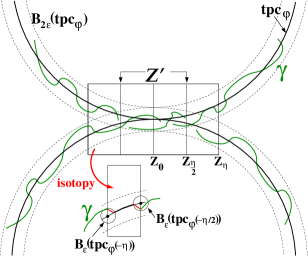
Figure 4.1: The handle isotopy on $\mathcal{Z}$: an intermediate stage, where one connects the part of $\operatorname{tpc}_{\varphi}$ in $\mathcal{Z}\setminus\mathcal{Z^{\prime}}$ to $\gamma$ by short straight segments.

Lemma 4.3 (Handle isotopy).

Let $\varphi\in(0,\pi]$, $\zeta\in\left(0,\tfrac{1}{96\pi}\right]$, and $\gamma\in C^{1}(\mathbb{R}/\mathbb{Z},\mathbb{R}^{3})$ with

$$\left\|\gamma-\operatorname{tpc}_{\varphi}\right\|_{C^{1}}\leq\delta\equiv\delta_{\varepsilon}$$

where $\delta_{\varepsilon}>0$ is the constant from (4.5) and

$$\varepsilon\equiv\varepsilon_{\zeta}:=\min\left(\nicefrac{{\zeta}}{{64}}\sin\nicefrac{{\varphi}}{{2}},\tfrac{1}{20}\sqrt{\nicefrac{{\zeta}}{{8\pi}}}\right).$$ (4.12)

Then there is an isotopy of $B_{2\varepsilon}\left(\operatorname{tpc}_{\varphi}\right)$ which

• leaves $\mathcal{Z}^{\prime}$ and $\partial B_{2\varepsilon}\left(\operatorname{tpc}_{\varphi}\right)$ pointwise fixed,

• deforms $\gamma\setminus\mathcal{Z}$ to $\operatorname{tpc}_{\varphi}\setminus\mathcal{Z}$, and

• moves points by at most $4\varepsilon$.

Remark 4.4.

From the proof it will become clear that the isotopy actually deforms all of $\gamma$ outside a small $\varepsilon$-neighbourhood $B_{\varepsilon}(\mathcal{Z}^{\prime})$ of the smaller cylinder $\mathcal{Z}^{\prime}$ to $\operatorname{tpc}_{\varphi}.$ In addition, in the small region $B_{\varepsilon}(\mathcal{Z}^{\prime})\setminus\mathcal{Z}^{\prime}$ the curve $\gamma$ is deformed into a straight segment that lies in the $2\varepsilon$-neighbourhood of $\operatorname{tpc}_{\varphi}$. $\Diamond$

Notice for the following proof that the $\varepsilon$-neighbourhood of $\operatorname{tpc}_{\varphi}$ coincides with the union of all $\varepsilon$-normal disks of $\operatorname{tpc}_{\varphi}$.

Proof 9.

On circular fibres we may employ an isotopy adapted from Crowell and Fox [10, App. I, p. 151]. For an arbitrary closed circular planar disk $D$ and given interior points $p_{0},p_{1}\in D$ we may define an homeomorphism $g_{D,p_{0},p_{1}}:D\to D$ by mapping any ray joining $p_{0}$ to a point $q$ on the boundary of $D$ linearly onto the ray joining $p_{1}$ to $q$ so that $p_{0}\mapsto p_{1}$ and $q\mapsto q$. This leaves the boundary $\partial D$ pointwise invariant. Furthermore, $g_{D,p_{0},p_{1}}$ is continuous in $p_{0}$, $p_{1}$ and $D$ (thus especially in the center and the radius of $D$). Of course, as $g_{D,p_{0},p_{1}}$ maps $D$ onto itself, any point is moved by at most the diameter of $D$. The isotopy is now provided by the homeomorphism

$$H:[0,1]\times D\to[0,1]\times D,\qquad(\lambda,x)\mapsto(\lambda,g_{D,p_{0},(1-\lambda)p_{0}+\lambda p_{1}}(x))$$ (4.13)

which analogously works for the ellipsoid.

Now we apply this isotopy to any fibre $\mathcal{Z}_{\xi}$ of

$$\mathcal{Z}\setminus\mathcal{Z}^{\prime}=\bigcup_{\left|\xi\right|\in[\eta/2,\eta]}\mathcal{Z}_{\xi}.$$

Here, for $j=1,2$ and any $\xi$ satisfying $\left|\xi\right|\in\left[\nicefrac{{\eta}}{{2}},\eta\right]$, we let $\left\{p_{0,j}\right\}=\mathcal{Z}_{\xi}\cap\tilde{\gamma}_{j}$ and $D_{j}$ be the $2\varepsilon$-ball centered at $p_{1,j}:=\widetilde{\operatorname{tpc}}_{\varphi,j}(\xi)$. As $\varepsilon<\nicefrac{{\zeta}}{{4}}$ we have $D_{j}\subset\mathcal{Z}_{\xi}$,

By our choice of $\varepsilon$, the disks $D_{1}$ and $D_{2}$ in each fibre are disjoint. To see this, we compute using $1-\cos\varphi=2\sin^{2}\nicefrac{{\varphi}}{{2}}$

$$\begin{split}\left|\widetilde{\operatorname{tpc}}_{\varphi,1}(\xi)-\widetilde{\operatorname{tpc}}_{\varphi,2}(\xi)\right|&=\tfrac{1}{4\pi}\left(1-\cos\arcsin(4\pi\xi)\right)\sqrt{2-2\cos\varphi}\\ &=\tfrac{1}{4\pi}\left(1-\sqrt{1-(4\pi\xi)^{2}}\right)\cdot 2\sin\nicefrac{{\varphi}}{{2}}\\ &=\frac{(4\pi\xi)^{2}}{1+\sqrt{1-(4\pi\xi)^{2}}}\cdot\frac{\sin\tfrac{\varphi}{2}}{2\pi}\geq 4\pi\xi^{2}\sin\nicefrac{{\varphi}}{{2}}\\ &\geq\pi\eta^{2}\sin\nicefrac{{\varphi}}{{2}}=\nicefrac{{\zeta}}{{8}}\sin\nicefrac{{\varphi}}{{2}}\geq 8\varepsilon\end{split}$$ (4.14)

for any $\xi\in\left[\nicefrac{{\eta}}{{2}},\eta\right]$, so $\operatorname{dist}(D_{1},D_{2})\geq 8\varepsilon-2\cdot 2\varepsilon=4\varepsilon>0$.

Now we construct an isotopy on the fibres contained in $\mathcal{Z}\setminus\mathcal{Z}^{\prime}$, see Figure 4.1. We will always employ the isotopy (4.13) on the fibres with $p_{0,j}:=\tilde{\gamma}_{j}(\xi)$.

For $\xi\in\left[\nicefrac{{\eta}}{{2}},\nicefrac{{\eta}}{{2}}+\varepsilon\right]$ we let $p_{1,j}$ be the intersection of $\mathcal{Z}_{\xi}$ with the straight line joining $\tilde{\gamma}_{j}(\nicefrac{{\eta}}{{2}})$ and $\widetilde{\operatorname{tpc}}_{\varphi,j}(\nicefrac{{\eta}}{{2}}+\varepsilon)$. To this end we have to ensure that this line belongs to the $2\varepsilon$-neighborhood of $\operatorname{tpc}_{\varphi}$. (In fact, its interior points belong to $\mathcal{Z}\setminus\mathcal{Z}^{\prime}$ since any cylinder is convex.) As $\tilde{\gamma}_{j}(\nicefrac{{\eta}}{{2}})$ belongs to the $\varepsilon$-neighborhood of $\operatorname{tpc}_{\varphi}$, it is sufficient to apply Lemma 4.5 below. To this end, we let $f=\mathbb{P}\,\widetilde{\operatorname{tpc}}_{\varphi,j}$ where $\mathbb{P}$ denotes the projection to $\mathbf{e}_{2}^{\perp}$, and

$$f^{\prime}(\xi)=\frac{\mathbb{P}\operatorname{tpc}_{\varphi}^{\prime}\left(\frac{\arcsin(4\pi\xi)}{4\pi}\right)}{\sqrt{1-(4\pi\xi)^{2}}},\quad f^{\prime\prime}(\xi)=\frac{\mathbb{P}\operatorname{tpc}_{\varphi}^{\prime\prime}\left(\frac{\arcsin(4\pi\xi)}{4\pi}\right)}{{1-(4\pi\xi)^{2}}}+(4\pi)^{2}\xi\frac{\mathbb{P}\operatorname{tpc}_{\varphi}^{\prime}\left(\frac{\arcsin(4\pi\xi)}{4\pi}\right)}{\left(1-(4\pi\xi)^{2}\right)^{3/2}}.$$

As $\left|\operatorname{tpc}_{\varphi}^{\prime}\right|\equiv 1$, $\left|\operatorname{tpc}_{\varphi}^{\prime\prime}\right|\equiv 4\pi$ (up to the points $t=0$, $t=\tfrac{1}{2}$ of tangential intersection), we arrive at $\left|f^{\prime\prime}\right|\leq 6\pi$ for any $\xi\in\left[-\frac{1}{16\pi},\frac{1}{16\pi}\right]$. Then, applying Lemma 4.5 to $f(\cdot-\nicefrac{{\eta}}{{2}})$ with $\ell=\varepsilon$, $K=6\pi$, and $y=\tilde{\gamma}_{j}(\nicefrac{{\eta}}{{2}})$, the distance of any point of the straight line to $f$ is bounded by $\sqrt{2}\cdot 6\pi\varepsilon^{2}+\varepsilon<2\varepsilon$ for $\varepsilon<\frac{1}{6\pi\sqrt{2}}$. For future reference we remark that, by $\left|\widetilde{\operatorname{tpc}}^{\prime}_{\varphi,j}\right|\leq\nicefrac{{4}}{{\sqrt{15}}}$, the angle between the straight line and the $\mathbf{e}_{2}$-axis is bounded above by

$$\arctan\frac{\left|\tilde{\gamma}_{j}(\nicefrac{{\eta}}{{2}})-\widetilde{\operatorname{tpc}}_{\varphi,j}(\nicefrac{{\eta}}{{2}})\right|+\left|\widetilde{\operatorname{tpc}}_{\varphi,j}(\nicefrac{{\eta}}{{2}})-\widetilde{\operatorname{tpc}}_{\varphi,j}(\nicefrac{{\eta}}{{2}}+\varepsilon)\right|}{\left(\nicefrac{{\eta}}{{2}}+\varepsilon\right)-\nicefrac{{\eta}}{{2}}}\leq\arctan\tfrac{\varepsilon+4\varepsilon/\sqrt{15}}{\varepsilon}<\tfrac{2}{5}\pi.$$ (4.15)

For $\xi\in\left[\nicefrac{{\eta}}{{2}}+\varepsilon,\eta-\varepsilon\right]$ we let $p_{1,j}=\widetilde{\operatorname{tpc}}_{\varphi,j}(\xi)$.

For $\xi\in\left[\eta-\varepsilon,\eta\right]$ we let $p_{1,j}$ be the intersection of $\mathcal{Z}_{\xi}$ with the straight line joining $\tilde{\gamma}_{j}(\eta)$ and $\widetilde{\operatorname{tpc}}_{\varphi,j}(\eta-\varepsilon)$. We argue as before using Lemma 4.5. This particular straight line ends at one cap of $\mathcal{Z}$ and will be moved to $\operatorname{tpc}_{\varphi}$ by the second isotopy.

The same construction can be applied for the corresponding negative values of $\xi$. Now we have obtained the situation sketched in Figure 4.1.

We consider the $2\varepsilon$-neighborhood of $\operatorname{tpc}_{\varphi}$. It consists of normal disks centered at the points of $\operatorname{tpc}_{\varphi}$. We restrict to a neighborhood containing those normal disks that do not intersect $\mathcal{Z}^{\prime}$. They cover the straight lines in $\mathcal{Z}$ at $\left|\xi\right|\in\left[\eta-\varepsilon,\eta\right]$ for otherwise there would be some normal disk (of radius $2\varepsilon$) intersecting the straight line (at $\left|\xi\right|\in[\eta-\varepsilon,\eta]$) and $\mathcal{Z}^{\prime}$ (at $\xi\in[-\nicefrac{{\eta}}{{2}},\nicefrac{{\eta}}{{2}}]$). However, by construction, $(\eta-\varepsilon)-\nicefrac{{\eta}}{{2}}=\nicefrac{{\eta}}{{2}}-\varepsilon=\tfrac{1}{2}\sqrt{\nicefrac{{\zeta}}{{8\pi}}}-\varepsilon\stackrel{{\scriptstyle\text{\makebox[0.0pt][c]{\eqref{eq:epsilon}}}}}{{\geq}}9\varepsilon$, a contradiction.

In order to apply the isotopy which moves the points of $\gamma$ to $\operatorname{tpc}_{\varphi}$, we have to show that all points of $\gamma$ (and the straight lines as well) belong to the $2\varepsilon$-neighborhood of $\operatorname{tpc}_{\varphi}$ and transversally meet the corresponding normal disk.

For the straight lines we have already seen (using Lemma 4.5) that they lie inside the $2\varepsilon$-neighborhood of $\operatorname{tpc}_{\varphi}$. On $\left|\xi\right|\leq\eta\leq\frac{1}{\sqrt{3}\cdot 16\pi}$ the angle $\alpha$ between the $\mathbf{e}_{2}$-axis and the tangent line to $\widetilde{\operatorname{tpc}}_{\varphi,j}$ amounts at most to

$$\arcsin\frac{\frac{1}{16\pi\sqrt{3}}}{\frac{1}{4\pi}}=\arcsin\tfrac{1}{4\sqrt{3}}<\tfrac{\pi}{10};$$ (4.16)

see Figure 4.2.

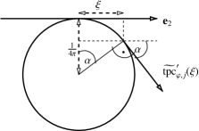
Figure 4.2: Elementary geometry leading to (4.16): $\sin\alpha\leq 4\pi\xi\leq\tfrac{4\pi}{16\sqrt{3}\pi}=\tfrac{1}{4\sqrt{3}}$.

Therefore, using (4.15), the angle between the straight line and the tangent line to $\widetilde{\operatorname{tpc}}_{\varphi,j}$ is strictly smaller than $\frac{\pi}{2}$, which implies transversality.

As calculated above, the distance between $\mathcal{Z}_{\eta}$ and $\mathcal{Z}_{\eta/2}$ amounts to at least $10\varepsilon$, so the straight line is covered by normal disks which do not intersect $\mathcal{Z}^{\prime}$.

For the other points of $\gamma$ outside $\mathcal{Z}$ we argue as in (4.11). $\Box$

Lemma 4.5 (Lines inside a graphical tubular neighborhood).

Let $f\in C^{2}([0,\ell],\mathbb{R}^{d})$, $\left|f^{\prime\prime}\right|\leq K$, $y\in\mathbb{R}^{d}$. Then, $g(x):=f(x)-\left(f(0)+\frac{x}{\ell}(y-f(0))\right)$ satisfies

$$\left|g(x)\right|\leq\sqrt{d}K\ell^{2}+\left|y-f(\ell)\right|\qquad\text{for any }x\in[0,\ell].$$

Proof 10.

We compute

$$g(x)=\int_{0}^{x}\left(f^{\prime}(\xi)-\frac{f(\ell)-f(0)}{\ell}-\frac{y-f(\ell)}{\ell}\right)\,\mathrm{d}\xi.$$

By the mean value theorem, there are $\sigma_{1},\dots,\sigma_{d}\in(0,\ell)$ with $f^{\prime}_{j}(\sigma_{j})=\frac{f_{j}(\ell)-f_{j}(0)}{\ell}$, $j=1,\dots,d$, so

$$\left|g(x)\right| \leq\int_{0}^{x}\sqrt{\left|f^{\prime}_{1}(\xi)-f^{\prime}_{1}(\sigma_{1})\right|^{2}+\cdots+\left|f^{\prime}_{d}(\xi)-f^{\prime}_{d}(\sigma_{d})\right|^{2}}\,\mathrm{d}\xi+\left|y-f(\ell)\right|$$

$$\leq\sqrt{d}K\ell^{2}+\left|y-f(\ell)\right|.$$

$\Box$

Recall the definition of the continuous accumulating angle function $\beta:[-\eta,\eta]\to\mathbb{R}$ in (4.4), and $\Delta_{\beta}=\beta(\eta)-\beta(-\eta)$, where $a_{\xi}$ is the segment connecting $\tilde{\gamma}_{1}(\xi)$ and $\tilde{\gamma}_{2}(\xi)$ (see (4.2)), and $\nu$ was given by (4.3).

Proposition 4.6 (Only $(2,b)$-torus knots are $C^{1}$-close to $\operatorname{tpc}_{\varphi}$).

Let $\varphi\in(0,\pi]$, $\zeta\in\left(0,\tfrac{1}{96\pi}\right]$, and $\gamma\in C^{1}(\mathbb{R}/\mathbb{Z},\mathbb{R}^{3})$ be embedded with

$$\left\|\gamma-\operatorname{tpc}_{\varphi}\right\|_{C^{1}}\leq\delta$$

where $\delta\equiv\delta_{\varepsilon}>0$ and $\varepsilon\equiv\varepsilon_{\zeta}>0$ are defined in (4.5) and (4.12). Let $b\in\mathbb{Z}$ denote the rounded value of $\Delta_{\beta}/\pi$. Then $b$ is an odd integer, and $\gamma$ is unknotted if $b=\pm 1$ and belongs to $\mathcal{T}({2,b})$, if $|b|\geq 3.$

Figure 4.3: The maximal possible angle between the lines defined by $a_{\pm\xi}$ and $\nu$.

Proof 11.

For each $\xi\in[\eta/2,\eta]$ (in fact, for any $\xi\in(0,\eta]$) the line $\mathbb{R}\nu$ is perpendicular to the vectors $\chi_{\pm\xi}:=\widetilde{\operatorname{tpc}}_{\varphi,1}(\pm\xi)-\widetilde{\operatorname{tpc}}_{\varphi,2}(\pm\xi)$, and notice that $\chi_{\xi}=-\chi_{-\xi}$.

The endpoints $\tilde{\gamma}_{1}(\pm\xi)$ and $\tilde{\gamma}_{2}(\pm\xi)$ of the vectors $a_{\pm\xi}$ are contained in disks of radius $2\varepsilon$ inside $\mathcal{Z}_{\pm\xi}$ centered at $\widetilde{\operatorname{tpc}}_{\varphi,j}(\pm\xi)$, $j=1,2$, for $\xi\in[\eta/2,\eta]$. According to (4.14), these disks are disjoint, having distance at least $4\varepsilon$, so that the usual (unoriented) angle between $\chi_{\pm\xi}$ and $a_{\pm\xi}$ is bounded by $\arcsin\frac{2\varepsilon}{4\varepsilon}=\frac{\pi}{6}$, see Figure 4.3. Consequently,

$$\mathop{\mbox{$<\!\!\!)\,$}}\nolimits(\nu,a_{\xi})\in[\tfrac{\pi}{2}-\tfrac{\pi}{6},\tfrac{\pi}{2}+\tfrac{\pi}{6}]\quad{\textnormal{for all\,\,}}|\xi|\in[\tfrac{\eta}{2},\eta];$$

hence, according to (4.4), $\beta(-\eta)\in[\tfrac{3\pi}{2}-\tfrac{\pi}{6},-\tfrac{3\pi}{2}+\tfrac{\pi}{6}]$. For the range $\xi\in[\eta/2,\eta]$ such an explicit statement about $\beta(\xi)$ (taking values in $\mathbb{R}$) cannot be made, since the vector $a_{\xi}$ may have rotated several times while $\xi$ traverses the interval $[-\eta/2,\eta/2]$, but the vector $a_{\xi}$ points roughly into the direction of $\chi_{\xi}$ for each $\xi\in[\eta/2,\eta]$, which implies that there is an integer $m\in\mathbb{Z}$ (counting those rotations) such that

$$(2m+1)\pi-\tfrac{\pi}{3}\leq\beta(\xi)-\beta(-\xi)\leq(2m+1)\pi+\tfrac{\pi}{3}\quad{\textnormal{for all\,\,}}\xi\in[\eta/2,\eta].$$

This in turn yields that the rounded value of $(\beta(\xi)-\beta(-\xi))/\pi$ for all $\xi\in[\eta/2,\eta)$, and hence also $b$ equals $(2m+1)$, an odd number.

Therefore, in order to determine the knot type of $\gamma$, we may apply Lemma 4.3 to deform $\gamma$ into an ambient isotopic curve $\gamma_{*}$ and analyze that curve instead. By Remark 4.4 the previous arguments apply to $\gamma_{*}$ as well, in particular the crucial angle-estimate based on Figure 4.3. So the rounded value $b_{*}$ of $\Delta_{\beta_{*}}$ of the angle $\beta_{*}(\xi)$ defined by $\mathbf{e}_{1}\cos\left(\nicefrac{{\varphi}}{{2}}+\beta_{*}(\xi)\right)+\mathbf{e}_{3}\sin\left(\nicefrac{{\varphi}}{{2}}+\beta_{*}(\xi)\right)=a_{*\xi}:=\tilde{\gamma}_{*1}(\xi)-\tilde{\gamma}_{*2}(\xi)$ coincides with $b$, since $\gamma_{*}$ coincides with $\gamma$ in the subcylinder $\mathcal{Z}^{\prime}$. (By construction we know (see Lemma 4.3 and Remark 4.4) that $\gamma_{*}\cap\mathcal{Z}$ consists of two sub-arcs of $\gamma_{*}$ transversally meeting each fibre $\mathcal{Z}_{\xi}$, $\xi\in[-\eta,\eta]$, of the cylinder $\mathcal{Z}$, so the vectors $a^{*}_{\xi}$ are well-defined.)

We may now consider the $C^{1}$-mapping $\mathfrak{n}:[-\nicefrac{{\eta}}{{2}},\nicefrac{{\eta}}{{2}}]\to\mathbb{S}^{1}$, $\xi\mapsto\frac{a^{*}_{\xi}}{\left|a^{*}_{\xi}\right|}\in{\textnormal{span\,}}\{\mathbf{e}_{1},\mathbf{e}_{3}\}$. By Sard’s theorem, almost any direction $\tilde{\nu}\in\mathbb{S}^{1}$ is a regular value of $\mathfrak{n}$, i.e., its preimage consists of isolated (thus, by compactness, finitely many) points $-\nicefrac{{\eta}}{{2}}\leq\xi_{1}<\cdots<\xi_{k}\leq\nicefrac{{\eta}}{{2}}$ (so-called regular points) at which the derivative of $\mathfrak{n}$ does not vanish. At these points we face a self-intersection of the two strands inside $\mathcal{Z}$ when projecting onto $\tilde{\nu}^{\perp}$. Due to $\mathfrak{n}^{\prime}(\xi_{j})\neq 0$, $j=1,\dots,k$, each of these points can be identified to be either an overcrossing () or an undercrossing (). We choose some $\psi\in\mathbb{R}/2\pi\mathbb{Z}$ arbitrarily close to $\nicefrac{{\varphi}}{{2}}$, such that

$$\tilde{\nu}=\mathbf{e}_{1}\cos\psi+\mathbf{e}_{3}\sin\psi$$

is a regular value of $\mathfrak{n}$.

As $\gamma_{*}$ coincides with $\operatorname{tpc}_{\varphi}$ outside $\mathcal{Z}$ and $a^{*}_{\xi}/\left|a^{*}_{\xi}\right|$ is bounded away from the projection line $\mathbb{R}\tilde{\nu}$, i.e., $\mathop{\mbox{$<\!\!\!)\,$}}\nolimits(a^{*}_{\xi},\nu)\in[\nicefrac{{\pi}}{{2}}-\nicefrac{{\pi}}{{6}},\nicefrac{{\pi}}{{2}}+\nicefrac{{\pi}}{{6}}]$, for all $\left|\xi\right|\in[\nicefrac{{\eta}}{{2}},\eta]$ there are no crossings outside $\mathcal{Z}^{\prime}$.

In fact, the projection provides a two-braid presentation of the knot as we see two strands transversally passing through the fibres of a narrow cylinder in the same direction. This is a (two-) braid. The fact that the strands’ end-points on one cap of the cylinder are connected to the end-points on the opposite cap by two “unlinked” arcs (outside $\mathcal{Z}^{\prime}$) provides a closure of the braid.

The isotopy class of any braid consisting of $n$ strands is uniquely characterized by a braid word, i.e., an element of the group $\mathcal{B}_{n}$ which is given by $n-1$ generators $\sigma_{1},\dots,\sigma_{n-1}$ and the relations

$$\begin{split}\sigma_{j}\sigma_{j+1}\sigma_{j}=\sigma_{j+1}\sigma_{j}\sigma_{j+1}&\quad\text{for }j=1,\dots,n-2,\\ \text{and}\qquad\sigma_{j}\sigma_{k}=\sigma_{k}\sigma_{j}&\quad\text{for }1,\dots,j<k-1,\dots,n-2,\end{split}$$ (4.17)

see Burde and Zieschang [9, Prop. 10.2, 10.3]. Closures of braids (resulting in knots or links) are ambient isotopic if and only if the braids are Markov equivalent. The latter means that the braids are connected by a finite sequence of braids where two consecutive braids are either conjugate or related by a Markov move, see [9, Def. 10.21, Thm. 10.22]. The latter replaces $\mathfrak{z}\in\mathcal{B}_{n-1}$ by $\mathfrak{z}\sigma_{n-1}^{\pm 1}$.

In the special case of two braids this condition simplifies as follows. As $\mathcal{B}_{2}$ has only one generator, namely with $(\overcrossing)^{-1}=\undercrossing$, in fact $\mathcal{B}_{2}\cong\mathbb{Z}$, conjugate braids are identical. As $\mathcal{B}_{1}=\left\{1\right\}$, a Markov move can only be applied to the word $1$, thus proving that the closed one-braid, i.e., the round circle, is ambient isotopic to the closures of both and , which settles the case $b=b_{*}=\pm 1.$

Assume now $|b|\geq 3$. The braid represented by $\tilde{\gamma}_{1}$ and $\tilde{\gamma}_{2}$ is characterized by the braid word $(\overcrossing)^{k}$ for some $k\in\mathbb{Z}$. If $k$ were even we would arrive at a two-component link which is impossible. Any overcrossing is equivalent to half a rotation of $a_{\xi}$ in positive direction (with respect to the $\mathbf{e}_{1}$-$\mathbf{e}_{3}$-plane). This gives $k=b$. On the other hand, one easily checks from (5.1) that a $(2,b)$-torus knot has the braid word $\sigma_{1}^{-b}$, $b\in 1+2\mathbb{Z}$, $b\neq\pm 1$ (cf. Artin [1, p. 56]). $\Box$

Corollary 4.7 (Torus knots).

Any embedded $\gamma\in C^{1}(\mathbb{R}/\mathbb{Z},\mathbb{R}^{3})$ with $\left\|\gamma-\operatorname{tpc}_{0}\right\|_{C^{1}}\leq\tfrac{1}{100}$ is either unknotted or belongs to $\mathcal{T}({2,b})$ for some odd $b\neq\pm 1$.

Sketch of proof 1.

We argue similarly to the preceding argument. The image of $\operatorname{tpc}_{0}$ coincides with the circle of radius $\nicefrac{{1}}{{4\pi}}$ in the $\mathbf{e}_{1}$-$\mathbf{e}_{2}$-plane centered at $\nicefrac{{\mathbf{e}_{1}}}{{8\pi}}$. Consider the $\frac{1}{100}$-neighborhood of $\operatorname{tpc}_{0}$ fibred by the normal disks of this circle. Any of these normal disks is transversally met by $\gamma$ in precisely two points. Consider the Gauß map $\mathfrak{n}:\mathbb{R}/\mathbb{Z}\times\mathbb{R}/\mathbb{Z}\to\mathbb{S}^{2}$, $(s,t)\mapsto\frac{\gamma(s)-\gamma(t)}{\left|\gamma(s)-\gamma(t)\right|}$. Off the diagonal, this map is well-defined and $C^{1}$. Sard’s lemma gives the existence of some $\nu_{0}\in\mathbb{S}^{2}$ arbitrarily close to $\mathbf{e}_{3}$, such that any crossing of $\gamma$ in the projection onto $\nu_{0}^{\perp}$ is either an over- or an undercrossing. Here we face the situation of a deformed cylinder with its caps glued together. By stretching and deforming, we arrive at a usual braid representation. We conclude as before. “$\Box$”

5 Comparison $(2,b)$-torus knots and energy estimates

Let $a,b\in\mathbb{Z}\setminus\left\{-1,0,1\right\}$ be coprime, i.e., $\gcd(\left|a\right|,\left|b\right|)=1$. The $(a,b)$-torus knot class $\mathcal{T}({a,b})$ contains the one-parameter family of curves

$$\tau_{\varrho}:t\mapsto\begin{pmatrix}(1+\varrho\cos(bt))\cos(at)\\ (1+\varrho\cos(bt))\sin(at)\\ \varrho\sin(bt)\end{pmatrix},\quad t\in\mathbb{R}/2\pi\mathbb{Z},$$ (5.1)

where the parameter $\varrho\in(0,1)$ can be chosen arbitrarily. For information on torus knots we refer to Burde and Zieschang [9, Chapters 3 E, 6]. As $\mathcal{T}({-a,b})=\mathcal{T}({a,-b})$ [9, Prop. 3.27], it suffices to consider $a>1$. Since $\mathcal{T}({a,-b})$ contains the mirror images of $\mathcal{T}({a,b})$ we may also, keeping in mind this symmetry, pass to $b>1$. Note, however, that the latter classes are in fact disjoint, i.e., torus knots are not amphicheiral [9, Thm. 3.29].

We will later restrict to $a=2$; in this case $\gcd(2,b)=1$ holds for any odd $b$ with $|b|\geq 3$. The two (mirror-symmetric) trefoil knot classes coincide with the $(2,\pm 3)$-torus knot classes.

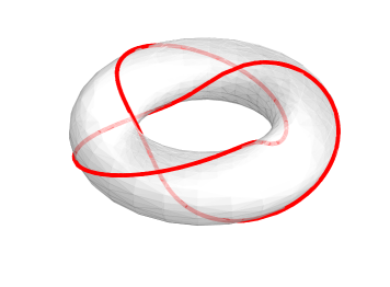
Figure 5.1: Plot of $\tau_{1/3}$ for the trefoil knot class $\mathcal{T}({2,3})$

The total curvature of a given curve $\gamma\in H^{2}(\mathbb{R}/L\mathbb{Z},\mathbb{R}^{3})$, $L>0$, is given by

$$\operatorname{TC}(\gamma)=\int_{\gamma}\varkappa\,\mathrm{d}s=\int_{\mathbb{R}/L\mathbb{Z}}{\varkappa}\left|\gamma^{\prime}\right|\,\mathrm{d}t=\int_{0}^{L}\frac{\left|\gamma^{\prime\prime}\wedge\gamma^{\prime}\right|}{\left|\gamma^{\prime}\right|^{2}}\,\mathrm{d}t\stackrel{{\scriptstyle\left|\gamma^{\prime}\right|\equiv 1}}{{=}}\int_{0}^{L}{\left|\gamma^{\prime\prime}\right|}\,\mathrm{d}t.$$ (5.2)

The torus knots $\tau_{\varrho}$ introduced in (5.1) lead to a family of comparison curves that approximate the $a$-times covered circle $\tau_{0}$ with respect to the $C^{k}$-norm for any $k\in\mathbb{N}$ as $\varrho\searrow 0$. Rescaling and reparametrizing to arc-length we obtain $\tilde{\tau}_{\varrho}\in\mathscr{C}({{\mathcal{T}({a,b})}})$. As this does not destroy $H^{2}$-convergence [28, Thm. A.1], we find that the arclength parametrization $\tilde{\tau}_{0}$ of the $a$-times covered circle lies in the (strong) $H^{2}$-closure of $\mathscr{C}({{\mathcal{T}({a,b})}})$.

Lemma 5.1 (Bending energy estimate for comparison torus knots).

There is a constant $C=C(a,b)$ such that

$$E_{\mathrm{bend}}(\tilde{\tau}_{\varrho})\leq(2\pi a)^{2}+C\varrho^{2}\qquad\text{for all }\varrho\in\left[0,\tfrac{a}{4\sqrt{a^{2}+b^{2}}}\right]\,.$$ (5.3)

Proof 12.

We begin with computing the first derivatives of $\tau_{\varrho}$,

$$\tau_{\varrho}^{\prime}(t) =\begin{pmatrix}-b\varrho\sin(bt)\cos(at)-a(1+\varrho\cos(bt))\sin(at)\\ -b\varrho\sin(bt)\sin(at)+a(1+\varrho\cos(bt))\cos(at)\\ b\varrho\cos(bt)\end{pmatrix},$$

$$\tau_{\varrho}^{\prime\prime}(t) =-\begin{pmatrix}\left(a^{2}+(a^{2}+b^{2})\varrho\cos(bt)\right)\cos(at)-2ab\varrho\sin(bt)\sin(at)\\ \left(a^{2}+(a^{2}+b^{2})\varrho\cos(bt)\right)\sin(at)+2ab\varrho\sin(bt)\cos(at)\\ b^{2}\varrho\sin(bt)\end{pmatrix},$$

$$\left|\tau_{\varrho}^{\prime}(t)\right|^{2} =b^{2}\varrho^{2}+a^{2}\left(1+\varrho\cos(bt)\right)^{2}$$

$$=a^{2}+2a^{2}\cos(bt)\varrho+\left(b^{2}+a^{2}\cos^{2}(bt)\right)\varrho^{2},$$ (5.4)

$$\left|\tau_{\varrho}^{\prime\prime}(t)\right|^{2} =a^{4}+2a^{2}(a^{2}+b^{2})\cos(bt)\varrho+\left[(4a^{2}+b^{2})b^{2}+a^{2}(a^{2}-2b^{2})\cos^{2}(bt)\right]\varrho^{2},$$

$$\left\langle\tau_{\varrho}^{\prime\prime}(t),\tau_{\varrho}^{\prime}(t)\right\rangle =-a^{2}b\varrho\sin(bt)\left(1+\varrho\cos(bt)\right),$$

which by means of the Lagrange identity implies

$$E_{\mathrm{bend}}(\tau_{\varrho}) =\int_{0}^{2\pi}\frac{\left|\tau_{\varrho}^{\prime\prime}(t)\wedge\tau_{\varrho}^{\prime}(t)\right|^{2}}{\left|\tau_{\varrho}^{\prime}(t)\right|^{5}}\,\mathrm{d}t=\int_{0}^{2\pi}\frac{\left|\tau_{\varrho}^{\prime\prime}(t)\right|^{2}\left|\tau_{\varrho}^{\prime}(t)\right|^{2}-\left\langle\tau_{\varrho}^{\prime\prime}(t),\tau_{\varrho}^{\prime}(t)\right\rangle^{2}}{\left|\tau_{\varrho}^{\prime}(t)\right|^{5}}\,\mathrm{d}t$$

$$=\int_{0}^{2\pi}\left(\frac{\left|\tau_{\varrho}^{\prime\prime}(t)\right|^{2}}{\left|\tau_{\varrho}^{\prime}(t)\right|^{3}}-\frac{\left\langle\tau_{\varrho}^{\prime\prime}(t),\tau_{\varrho}^{\prime}(t)\right\rangle^{2}}{\left|\tau_{\varrho}^{\prime}(t)\right|^{5}}\right)\,\mathrm{d}t.$$

As

$$\left|\tau_{\varrho}^{\prime}(t)\right|^{2}\geq\tfrac{7}{16}a^{2}\quad\textnormal{ because $(a^{2}+b^{2})\varrho^{2}\leq\tfrac{1}{16}a^{2}$ and $2a^{2}\varrho\leq\tfrac{1}{2}a^{2}$}$$ (5.5)

the subtrahend in $E_{\mathrm{bend}}(\tau_{\varrho})$ and the third term in the expression for $|\tau_{\varrho}^{\prime\prime}|^{2}$ are bounded by $C\varrho^{2}$ uniformly in $t$. Expanding $z^{-3/2}=1-\tfrac{3}{2}z+\mathcal{O}(z^{2})$ as $z\to 0$ we derive

$$|\tau_{\varrho}^{\prime}(t)|^{-3}={\left(b^{2}\varrho^{2}+a^{2}\left(1+\varrho\cos(bt)\right)^{2}\right)^{-3/2}}=\frac{1}{a^{3}}-\frac{3}{a^{3}}\cos\left(bt\right)\varrho+\mathcal{O}(\varrho^{2}),$$

which yields

$$E_{\mathrm{bend}}(\tau_{\varrho})= \int_{0}^{2\pi}\left(a^{4}+2a^{2}(a^{2}+b^{2})\cos(bt)\varrho\right)\left(\frac{1}{a^{3}}-\frac{3}{a^{3}}\cos\left(bt\right)\varrho+\mathcal{O}(\varrho^{2})\right)\,\mathrm{d}t+\mathcal{O}(\varrho^{2})$$

$$= \int_{0}^{2\pi}\left(a+\tfrac{2b^{2}-a^{2}}{a}\cos\left(bt\right)\varrho\right)\,\mathrm{d}t+\mathcal{O}(\varrho^{2})=2\pi a+\mathcal{O}(\varrho^{2})\quad\textnormal{as $\varrho\searrow 0$.}$$

Finally, in order to pass to $\tilde{\tau}_{\varrho}$, we recall that $E_{\mathrm{bend}}$ is invariant under reparametrization and $E_{\mathrm{bend}}(r\gamma)=r^{-1}E_{\mathrm{bend}}(\gamma)$ for $r>0$. So the claim follows for $r:=\mathscr{L}(\tau_{\varrho})^{-1}$ by

$$\mathscr{L}(\tau_{\varrho}) =\int_{0}^{2\pi}\left|\tau_{\varrho}^{\prime}(t)\right|\,\mathrm{d}t=\int_{0}^{2\pi}\sqrt{b^{2}\varrho^{2}+a^{2}\left(1+\varrho\cos(bt)\right)^{2}}\,\mathrm{d}t$$

$$=\int_{0}^{2\pi}\left(a+a\cos(bt)\varrho+\mathcal{O}(\varrho^{2})\right)\,\mathrm{d}t=2\pi a+\mathcal{O}(\varrho^{2})\quad\textnormal{as $\varrho\to 0$.}$$

$\Box$

Proposition 5.2 (Ropelength estimate for comparison torus knots).

We have

$$\mathcal{R}(\tilde{\tau}_{\varrho})\leq\frac{C}{\varrho}\qquad\text{for }0<\varrho\ll 1,$$

where $C$ is a constant depending only on $a$ and $b$.

Proof 13.

The invariance of $\mathcal{R}$ under reparametrization, scaling, and translation implies $\mathcal{R}(\tilde{\tau}_{\varrho})=\mathcal{R}(\tau_{\varrho})$. According to Lemma 5.1 above, the squared curvature of $\tau_{\varrho}$ amounts to

$$\frac{\left|\tau_{\varrho}^{\prime\prime}(t)\wedge\tau_{\varrho}^{\prime}(t)\right|^{2}}{\left|\tau_{\varrho}^{\prime}(t)\right|^{6}}\leq\frac{\left|\tau_{\varrho}^{\prime\prime}(t)\right|^{2}}{\left|\tau_{\varrho}^{\prime}(t)\right|^{4}}$$

which is uniformly bounded independent of $\varrho$ and $t$ as long as $\varrho$ is in the range required in (5.3) by some $\varkappa_{0}>0$ (combine (5.4) with (5.5)). By $\mathscr{L}(\tau_{\varrho}|_{[s,t]})$ we denote the length of the shorter subarc of $\tau_{\varrho}$ connecting the points $\tau_{\varrho}(s)$ and $\tau_{\varrho}(t)$. As $\left|\tau_{\varrho}^{\prime}\right|$ uniformly converges to $a$ as $\varrho\to 0$ (see (5.4)), we may find some $\varrho_{0}\in\left(0,\tfrac{a}{4\sqrt{a^{2}+b^{2}}}\right]$ such that $a\left|s-t\right|_{\mathbb{R}/2\pi\mathbb{Z}}\geq\frac{1}{2}\mathscr{L}(\tau_{\varrho}|_{[s,t]})$ for any $\varrho\in(0,\varrho_{0}]$. The estimate

$$\left|\tau_{\varrho}(s)-\tau_{\varrho}(t)\right|\geq c\varrho\quad\text{for any }s,t\in\mathbb{R}/2\pi\mathbb{Z}\text{ with }\left|s-t\right|_{\mathbb{R}/2\pi\mathbb{Z}}\geq\tfrac{1}{20a\varkappa_{0}}\text{ and }\varrho\in(0,\varrho_{0}]$$ (5.6)

which will be proven below for some uniform $c>0$ now implies

$$\left|\tau_{\varrho}(s)-\tau_{\varrho}(t)\right|\geq c\varrho\quad\text{for any }s,t\in\mathbb{R}/2\pi\mathbb{Z}\text{ with }\mathscr{L}(\tau_{\varrho}|_{[s,t]})\geq\tfrac{1}{10\varkappa_{0}}\text{ and }\varrho\in(0,\varrho_{0}].$$

As $\mathscr{L}(\tau_{\varrho})$ is also uniformly bounded, we may apply Lemma 5.3 below, which yields the desired.

It remains to verify (5.6). Recall that the limit curve $\tau_{0}$ is an $a$-times covered circle parametrized by uniform speed $a$. Fix $t\in\mathbb{R}/2\pi\mathbb{Z}$ and consider the image of $\tau_{\varrho}(s)$ restricted to $s\in\mathbb{R}/2\pi\mathbb{Z}$ with $\left|s-t\right|_{\mathbb{R}/\frac{2\pi}{a}\mathbb{Z}}<\frac{\pi}{2ab}$, i.e. $s\in t+\frac{2\pi}{a}\mathbb{Z}+(-\frac{\pi}{2ab},\frac{\pi}{2ab})$, see Figure 5.2. It consists of $a$ disjoint arcs (on the $\varrho$-torus, in some neighborhood of $\tau_{0}(t)$). The associated angle function $s\mapsto bs$ (see (5.1)) strides across disjoint regions of length $\frac{\pi}{a}$ on $\mathbb{R}/2\pi\mathbb{Z}$ for each of those arcs. These regions have positive distance $\geq\frac{\pi}{a}$ on the surface of the $\varrho$-torus which leads to a uniform positive lower bound on $\frac{1}{\varrho}\left|\tau_{\varrho}(s)-\tau_{\varrho}(t)\right|$ for $s\in\mathbb{R}/2\pi\mathbb{Z}$ where $\left|s-t\right|_{\mathbb{R}/\frac{2\pi}{a}\mathbb{Z}}<\frac{\pi}{2ab}$ but $\left|s-t\right|_{\mathbb{R}/2\pi\mathbb{Z}}>\frac{\pi}{2ab}$. The latter restriction reflects the fact that each arc has zero distance to itself.

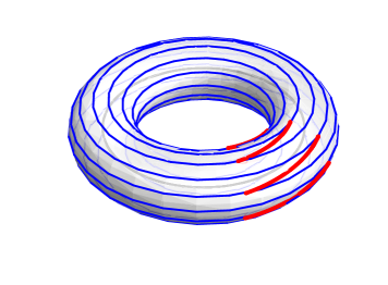
Figure 5.2: Plot of the regions of $\tau_{1/3}$ for $a=7$, $b=3$ (red; with respect to a fixed $t\in\mathbb{R}/\mathbb{Z}$) mentioned in the proof of Proposition 5.2. The blue lines visualize the (intrinsic) distance between the strands.

If, on the other hand, $\left|s-t\right|_{\mathbb{R}/\frac{2\pi}{a}\mathbb{Z}}\geq\lambda:=\min\left(\frac{\pi}{2ab},\frac{1}{20a\varkappa_{0}}\right)$, we may derive

$$\left|\tau_{\varrho}(s)-\tau_{\varrho}(t)\right|\geq\left|\tau_{0}(s)-\tau_{0}(t)\right|-2\varrho \geq 2\sin\left(\tfrac{a}{2}\left|s-t\right|_{\mathbb{R}/2\pi\mathbb{Z}}\right)-2\varrho_{0}$$

$$\geq 2\sin\left(\tfrac{a}{2}\left|s-t\right|_{\mathbb{R}/\frac{2\pi}{a}\mathbb{Z}}\right)-2\varrho_{0}\geq 2\sin{\tfrac{a\lambda}{2}}-2\varrho_{0}.$$

Diminishing $\varrho_{0}$ if necessary, the right-hand side is positive for all $\varrho\in(0,\varrho_{0}]$. $\Box$

Lemma 5.3 (Quantitative thickness bound).

Let $\gamma\in C^{2}(\mathbb{R}/\mathbb{Z},\mathbb{R}^{3})$ be a regular curve with uniformly bounded curvature $\varkappa\leq\varkappa_{0}$, $\varkappa_{0}>0$, and assume that

$$\delta:=\inf\left\{\left|\gamma(s)-\gamma(t)\right|\,\middle|\,s,t\in\mathbb{R}/\mathbb{Z},\mathscr{L}(\gamma|_{[s,t]})\geq\tfrac{1}{10\varkappa_{0}}\right\}$$

is positive where $\mathscr{L}(\gamma|_{[s,t]})$ denotes the length of the shorter sub-arc of $\gamma$ joining the points $\gamma(s)$ and $\gamma(t)$. Then $\triangle[\gamma]\geq\min\left(\tfrac{\delta}{2},\frac{1}{\varkappa_{0}}\right)>0$, thus

$$\mathcal{R}(\gamma)\leq{\max\left(\tfrac{2}{\delta},\varkappa_{0}\right)}{\mathscr{L}(\gamma)}<\infty.$$

Proof 14.

As the quantities in the statement do not depend on the actual parametrization and distances, thickness, and the reciprocal curvature are positively homogeneous of degree one, there is no loss of generality in assuming arc-length parametrization. According to [22, Thm. 1], the thickness equals the minimum of $\nicefrac{{1}}{{\max\varkappa}}\geq\nicefrac{{1}}{{\varkappa_{0}}}$ and one half of the doubly critical self-distance, that is, the infimum over all distances $\left|\gamma(s)-\gamma(t)\right|$ where $s,t\in\mathbb{R}/\mathbb{Z}$ satisfy $\gamma^{\prime}(s)\perp\gamma(s)-\gamma(t)\perp\gamma^{\prime}(t)$. By our assumption we only need to show that the doubly critical self-distance is not attained on the parameter range where $\mathscr{L}(\gamma|_{[s,t]})=\left|s-t\right|_{\mathbb{R}/\mathbb{Z}}<\tfrac{1}{10\varkappa_{0}}$.

To this end we show that any angle between $\gamma^{\prime}(t)$ and $\gamma(s)-\gamma(t)$ is smaller than $\frac{\pi}{6}<\frac{\pi}{2}$ if $\left|s-t\right|_{\mathbb{R}/\mathbb{Z}}\leq\tfrac{1}{10\varkappa_{0}}$. We obtain for $w:=\left|s-t\right|_{\mathbb{R}/\mathbb{Z}}\in\left[0,\frac{1}{10\varkappa_{0}}\right]$ (note that $\frac{1}{10\varkappa_{0}}<\frac{1}{2}$ by Fenchel’s theorem)

$$\left|\left\langle\gamma(s)-\gamma(t),\gamma^{\prime}(t)\right\rangle\right| =\left|(s-t)+(s-t)^{2}\int_{0}^{1}(1-\vartheta)\left\langle\gamma^{\prime\prime}(t+\vartheta(s-t)),\gamma^{\prime}(t)\right\rangle\,\mathrm{d}\vartheta\right|$$

$$\geq w\left(1-\varkappa_{0}w\right)\geq\tfrac{9}{10}w.$$

Using the Lipschitz continuity of $\gamma$, this yields for the angle $\alpha\in[0,\frac{\pi}{2}]$ between the lines parallel to $\gamma(s)-\gamma(t)$ and $\gamma^{\prime}(t)$

$$\cos\alpha=\frac{\left|\left\langle\gamma(s)-\gamma(t),\gamma^{\prime}(t)\right\rangle\right|}{\left|\gamma(s)-\gamma(t)\right|}\geq\tfrac{9}{10}>\tfrac{1}{2}\sqrt{3}=\cos\tfrac{\pi}{6}\qquad\Longrightarrow\qquad\alpha<\tfrac{\pi}{6}.$$

$\Box$

Combining Lemma 5.1 with the previous ropelength estimate we can use the comparison torus knots to obtain non-trivial growth estimates on the total energy $E_{\vartheta}$ and on the ropelength $\mathcal{R}$ of minimizers $\gamma_{\vartheta}$.

Proposition 5.4 (Total energy growth rate for minimizers).

For $a,b\in\mathbb{Z}\setminus\left\{-1,0,1\right\}$ with $\gcd(\left|a\right|,\left|b\right|)=1$ there is a positive constant $C=C(a,b)$ such that any sequence $\left(\gamma_{\vartheta}\right)_{{\vartheta>0}}$ of $E_{\vartheta}$-minimizers in $\mathscr{C}(\mathcal{T}(a,b))$ satisfies

$$E_{\vartheta}(\gamma_{\vartheta})\leq(2a\pi)^{2}+C{\vartheta^{2/3}}$$ (5.7)

and if $a=2$

$$\mathcal{R}(\gamma_{\vartheta})\leq C{\vartheta^{-1/3}}.$$ (5.8)

Proof 15.

The first claim immediately follows by $E_{\vartheta}(\gamma_{\vartheta})\leq E_{\vartheta}(\tilde{\tau}_{\vartheta^{1/3}})$ from Lemma 5.1 and Proposition 5.2. The classic Fáry–Milnor Theorem applied to $\gamma_{\vartheta}$ gives $(4\pi)^{2}+\vartheta\mathcal{R}(\gamma_{\vartheta})\leq E_{\vartheta}(\gamma_{\vartheta})$. Now the first estimate for $a=2$ implies the second one. $\Box$

6 Crookedness estimate and the elastic $(2,b)$-torus knot
Proofs of the main theorems

In his seminal article [24] on the Fáry–Milnor theorem, Milnor derived the lower bound for the total curvature of knotted arcs by studying the crookedness of a curve and relating it to the total curvature. For some regular curve $\gamma\in C^{0,1}(\mathbb{R}/\mathbb{Z},\mathbb{R}^{3})$, i.e., a Lipschitz-continuous mapping $\mathbb{R}/\mathbb{Z}\to\mathbb{R}^{d}$ which is not constant on any open subset of $\mathbb{R}/\mathbb{Z}$, the crookedness of $\gamma$ is the infimum over all $\nu\in\mathbb{S}^{2}$ of

$$\mu(\gamma,\nu):=\#\left\{t_{0}\in\mathbb{R}/\mathbb{Z}\,\middle|\,t_{0}\textnormal{ is a local maximizer of }t\mapsto\left\langle\gamma(t),\nu\right\rangle_{\mathbb{R}^{3}}\right\}.$$

We briefly cite the main properties, proofs can be found in [24, Sect. 3].

Proposition 6.1 (Crookedness).

Let $\gamma\in C^{0,1}(\mathbb{R}/\mathbb{Z},\mathbb{R}^{3})$ be a regular curve. Then

$$\operatorname{TC}(\gamma)=\tfrac{1}{2}\int_{\mathbb{S}^{2}}\mu(\gamma,\nu)\,\mathrm{d}\operatorname{\mathscr{H}^{2}}(\nu).$$

Any partition of $\mathbb{R}/\mathbb{Z}$ gives rise to an inscribed regular polygon $p\in C^{0,1}(\mathbb{R}/\mathbb{Z},\mathbb{R}^{3})$ with $\mu(p,\nu)\leq\mu(\gamma,\nu)$ for all directions $\nu\in\mathbb{S}^{2}$ that are not perpendicular to some edge of $p$.

The following statement is the heart of the argument for Theorem 1.1.

Lemma 6.2 (Crookedness estimate).

Let $\varphi\in(0,\pi]$,

$$\zeta:=\tfrac{1}{2}\min\left(\tfrac{1}{8\pi}\sin\nicefrac{{\varphi}}{{4}},\tfrac{1}{96\pi}\right),$$

and $\gamma\in C^{1,1}(\mathbb{R}/\mathbb{Z},\mathbb{R}^{3})$ be a non-trivially knotted, arclength parametrized curve with

$$\left\|\gamma-\operatorname{tpc}_{\varphi}\right\|_{C^{1}}\leq\delta$$ (6.1)

where $\delta\equiv\delta_{\varepsilon}>0$ and $\varepsilon\equiv\varepsilon_{\zeta}>0$ are defined in (4.5) and (4.12). Then the set

$$\mathcal{B}(\gamma):=\left\{\nu\in\mathbb{S}^{2}\,\middle|\,\mu(\gamma,\nu)\geq 3\right\}$$

is measurable with respect to the two-dimensional Hausdorff measure $\mathscr{H}^{2}$ on $\mathbb{S}^{2}$ and satisfies

$$\operatorname{\mathscr{H}^{2}}{(\mathcal{B}(\gamma))}\geq\tfrac{\pi}{16}\cdot\frac{\varphi}{\mathcal{R}(\gamma)}.$$

Proof 16.

As to the measurability of $\mathcal{B}(\gamma)$, we may consider the two-dimensional Hausdorff measure $\operatorname{\mathscr{H}^{2}}$ on $\mathbb{S}^{2}\setminus\mathscr{N}$ where $\mathscr{N}$ denotes the set of measure zero where $\mu(\gamma,\cdot)$ is infinite. From the fact that $\mu(\gamma,\cdot)$ is $\operatorname{\mathscr{H}^{2}}$-a.e. lower semi-continuous on $\mathbb{S}^{2}\setminus\mathscr{N}$ if $\gamma\in C^{1}$, we infer that $\left\{\nu\in\mathbb{S}^{2}\setminus\mathscr{N}\,\middle|\,\mu(\gamma,\nu)\leq 2\right\}$ is closed, thus measurable. Therefore, its complement (which coincides with $\mathcal{B}(\gamma)$ up to a set of measure zero) is also measurable.

As $\gamma$ is embedded and $C^{1,1}$, its thickness $\triangle[\gamma]=\nicefrac{{1}}{{\mathcal{R}(\gamma)}}$ is positive.

We consider the diffeomorphism $\Phi:(0,\pi)\times\mathbb{R}/2\pi\mathbb{Z}\to\mathbb{S}^{2}\setminus\left\{\pm\mathbf{e}_{2}\right\}$,

$$(\vartheta,\psi)\mapsto\begin{pmatrix}-\sin\vartheta\sin\psi\\ \cos\vartheta\\ \sin\vartheta\cos\psi\end{pmatrix}.$$

We aim at showing that, for a.e. $\psi\in[\nicefrac{{\varphi}}{{4}},\nicefrac{{3\varphi}}{{4}}]$, there is some sub-interval $J_{\psi}\subset(\tfrac{\pi}{6},\tfrac{5\pi}{6})$ with $\left|J_{\psi}\right|\geq\tfrac{\pi}{4}\triangle[\gamma]$ and $\Phi(\vartheta,\psi)\in\mathcal{B}(\gamma)$ for any $\vartheta\in J_{\psi}$. In this case we have

$$\operatorname{\mathscr{H}^{2}}(\mathcal{B}(\gamma))=\iint_{\mathbb{S}^{2}\setminus\left\{\pm\mathbf{e}_{2}\right\}}\chi_{\mathcal{B}(\gamma)}\,\mathrm{d}\operatorname{\mathscr{H}^{2}}=\int_{0}^{\pi}\int_{\mathbb{R}/2\pi\mathbb{Z}}\chi_{\Phi^{-1}(\mathcal{B}(\gamma))}\sin\vartheta\,\mathrm{d}\psi\,\mathrm{d}\vartheta\geq\tfrac{\pi}{16}\varphi\triangle[\gamma].$$

For given $\varphi\in(0,\pi]$ let

$$\tilde{\zeta}:=2\zeta=\min\left(\tfrac{1}{8\pi}\sin\nicefrac{{\varphi}}{{4}},\tfrac{1}{96\pi}\right)$$

and denote the corresponding cylinder by $\widetilde{\mathcal{Z}}$, cf. Section 4. For an arbitrary $\psi\in[\nicefrac{{\varphi}}{{4}},\nicefrac{{3\varphi}}{{4}}]$. The orthogonal projection onto $\nu_{\psi}^{\perp}$ for

$$\nu_{\psi}:=\cos\psi\mathbf{e}_{1}+\sin\psi\mathbf{e}_{3}=\Phi(\tfrac{\pi}{2},\psi-\tfrac{\pi}{2})$$

will be denoted by $\mathbb{P}_{\psi}$. Note that $\nu_{\psi}\perp\Phi(\vartheta,\psi)$ for any $\vartheta\in(0,\pi)$.

Firstly we note that the half circles $h$ of $\operatorname{tpc}_{\varphi}$ apart from the cylinder $\widetilde{\mathcal{Z}}$, namely $\operatorname{tpc}_{\varphi}$ restricted to $[\tfrac{1}{8},\tfrac{3}{8}]$ and $[\tfrac{5}{8},\tfrac{7}{8}]$ respectively, do not interfere with $\widetilde{\mathcal{Z}}$ when projected onto $\nu_{\psi}^{\perp}$, more precisely, $\mathbb{P}_{\psi}h\cap\mathbb{P}_{\psi}\widetilde{\mathcal{Z}}=\emptyset$. To see this, consider the projection $\Pi$ onto $\mathbf{e}_{2}^{\perp}$, see Figure 6.1. The two segments connecting $\operatorname{tpc}_{\varphi}(\tfrac{1}{8})$ to $\operatorname{tpc}_{\varphi}(\tfrac{3}{8})$, and $\operatorname{tpc}_{\varphi}(\tfrac{5}{8})$ to $\operatorname{tpc}_{\varphi}(\tfrac{7}{8})$, respectively, are mapped onto points $P,P^{\prime}\in\mathbf{e}_{2}^{\perp}$ under the projection $\Pi$, and $P$ and $P^{\prime}$ separate $\Pi(h)$ and $\Pi(\widetilde{\mathcal{Z}})$. From Figure 6.1 we read off that no projection line of $\mathbb{P}_{\psi}$ meets both $\mathcal{Z}$ and $h$, since otherwise, such a projection line (parallel to $\nu_{\psi}$ and orthogonal to $\mathbf{e}_{2}$ by definition) projected onto $\mathbf{e}_{2}^{\perp}$ under $\Pi$, would intersect both, $\Pi(\widetilde{\mathcal{Z}})$ and $\Pi(h)$, which is impossible.

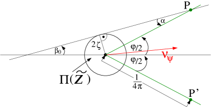
Figure 6.1: Under the projection $\Pi$ onto $\mathbf{e}_{2}^{\perp}$, the cylinder $\widetilde{\mathcal{Z}}$ is mapped to a disk. Each line enclosing an angle smaller than $\beta_{0}$ with $\nu$ cannot meet both this circle and (the line) $\Pi(h)$. Note that $\beta_{0}=\nicefrac{{\varphi}}{{2}}-\alpha$ and $\sin\alpha=8\pi\zeta\leq\tfrac{1}{2}\sin\nicefrac{{\varphi}}{{4}}<\sin\nicefrac{{\varphi}}{{4}}$, so $\alpha<\nicefrac{{\varphi}}{{4}}$ and $\beta_{0}>\nicefrac{{\varphi}}{{4}}$.

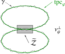
Figure 6.2: Projection onto $\nu_{\psi}^{\perp}$.

Now we consider the projection $\mathbb{P}_{\psi}$, see Figure 6.2. By construction there is (in the projection) one ellipse-shaped component on both sides of the line $\mathbb{R}\mathbf{e}_{2}$. As shown in (4.16), the angle between $\operatorname{tpc}_{\varphi}^{\prime}$ and $\mathbf{e}_{2}$ is bounded by $\tfrac{\pi}{10}$ on $|\xi|\leq\tfrac{1}{16\sqrt{3}\pi}$.

Proceeding as in (4.10) and using (6.1), we arrive at

$$\mathop{\mbox{$<\!\!\!)\,$}}\nolimits\left(\tilde{\gamma}_{j}^{\prime},\widetilde{\operatorname{tpc}}_{\varphi,j}^{\prime}\right) \leq\arccos\frac{\left\langle\tilde{\gamma}_{j}^{\prime},\widetilde{\operatorname{tpc}}_{\varphi,j}^{\prime}\right\rangle}{\left|\tilde{\gamma}_{j}^{\prime}\right|\left|\widetilde{\operatorname{tpc}}_{\varphi,j}^{\prime}\right|}\leq\arccos\frac{\left|\widetilde{\operatorname{tpc}}_{\varphi,j}^{\prime}\right|-\varepsilon}{\left|\widetilde{\operatorname{tpc}}_{\varphi,j}^{\prime}\right|+\varepsilon}\;\stackrel{{\scriptstyle\text{\makebox[0.0pt][c]{\eqref{eq:arccos-x}}}}}{{\leq}}\sqrt{\frac{2\pi\varepsilon}{\left|\widetilde{\operatorname{tpc}}_{\varphi,j}^{\prime}\right|+\varepsilon}}$$

$$\leq\sqrt{2\pi\varepsilon}\;\stackrel{{\scriptstyle\text{\makebox[0.0pt][c]{\eqref{eq:epsilon}}}}}{{\leq}}\sqrt{\tfrac{1}{10}\sqrt{\tfrac{1}{8\cdot 96}}}<0.1<\tfrac{\pi}{10},\qquad j=1,2.$$

Therefore the secant defined by two points of $\gamma$ inside $\widetilde{\mathcal{Z}}$, either both on $\tilde{\gamma}_{1}$, or both on $\tilde{\gamma}_{2}$, always encloses with $\mathbf{e}_{2}$ an angle of at most $\tfrac{\pi}{5}$, and the same holds true for the projection onto $\nu_{\psi}^{\perp}$.

Now we pass to the cylinder $\mathcal{Z}$ corresponding to $\zeta=\nicefrac{{\tilde{\zeta}}}{{2}}$. Note that the distance of $\partial\mathcal{Z}$ to $\partial\widetilde{\mathcal{Z}}$ is bounded below by $\min\left(\zeta,\left(\sqrt{2}-1\right)\sqrt{\nicefrac{{\zeta}}{{8\pi}}}\right)\geq\zeta$ and that

$$\zeta\geq\triangle[\gamma]$$ (6.2)

for otherwise the strands of $\gamma$ would not fit into $\mathcal{Z}$ which is guaranteed by Lemma 4.2.

Applying Proposition 4.6 (using Sard’s theorem) and assuming $b\geq 3$ (the case $b\leq-3$ being symmetric; recall that $b=\pm 1$ leads to the unknot) there are for a.e. $\psi\in[\nicefrac{{\varphi}}{{4}},\nicefrac{{3\varphi}}{{4}}]$ points

$$-\eta<\xi_{A}<\xi_{E}<\xi_{B}<\xi_{F}<\xi_{C}<\eta$$

such that $a_{\xi_{X}}$ is parallel to $\nu_{\psi}$ (thus $\mathbb{P}_{\psi}a_{\xi_{X}}=0$) for $X\in\left\{A,B,C\right\}$ while $a_{\xi_{X}}$ is perpendicular to $\nu_{\psi}$ for $X\in\left\{E,F\right\}$ and

$$\beta(\xi_{A})+\pi=\beta(\xi_{B})=\beta(\xi_{C})-\pi.$$

We claim

$$\left|a_{\xi_{E}}\right|,\left|a_{\xi_{F}}\right|\geq 2\triangle[\gamma].$$ (6.3)

To see this, consider the map $[-\eta,\eta]^{2}\to(0,1)$, $(\xi_{1},\xi_{2})\mapsto\left|\tilde{\gamma}_{1}(\xi_{1})-\tilde{\gamma}_{2}(\xi_{2})\right|$. There is at least one global minimizer $(\tilde{\xi}_{1},\tilde{\xi}_{2})$, and consequently we have $\tilde{\gamma}_{1}^{\prime}(\tilde{\xi}_{1})\perp\tilde{\gamma}_{1}(\tilde{\xi}_{1})-\tilde{\gamma}_{2}(\tilde{\xi}_{2})\perp\tilde{\gamma}_{2}^{\prime}(\tilde{\xi}_{2})$. For any $\tilde{}\varepsilon>0$ we may choose some $\tilde{\xi}_{\tilde{}\varepsilon}\in[-\eta,\eta]$ close to $\tilde{\xi}_{1}$ such that the radius $\tilde{}\varrho_{\tilde{}\varepsilon}$ of the circle passing through $\tilde{\gamma}_{1}(\tilde{\xi}_{1})$, $\tilde{\gamma}_{2}(\tilde{\xi}_{2})$, $\tilde{\gamma}_{1}(\tilde{\xi}_{\tilde{}\varepsilon})$ satisfies $\left|\tilde{\gamma}_{1}(\tilde{\xi}_{1})-\tilde{\gamma}_{2}(\tilde{\xi}_{2})\right|\geq 2\tilde{}\varrho_{\tilde{}\varepsilon}-\tilde{}\varepsilon\geq 2\triangle[\gamma]-\tilde{}\varepsilon$ (cf. Litherland et al. [22, Proof of Thm. 3]).

We let

$$A :=\mathbb{P}_{\psi}\tilde{\gamma}_{1}(\xi_{A})=\mathbb{P}_{\psi}\tilde{\gamma}_{2}(\xi_{A}), E :=\mathbb{P}_{\psi}\tilde{\gamma}_{1}(\xi_{E}), E^{\prime} :=\mathbb{P}_{\psi}\tilde{\gamma}_{2}(\xi_{E}),$$

$$B :=\mathbb{P}_{\psi}\tilde{\gamma}_{1}(\xi_{B})=\mathbb{P}_{\psi}\tilde{\gamma}_{2}(\xi_{B}), F :=\mathbb{P}_{\psi}\tilde{\gamma}_{1}(\xi_{F}), F^{\prime} :=\mathbb{P}_{\psi}\tilde{\gamma}_{2}(\xi_{F}),$$

$$C :=\mathbb{P}_{\psi}\tilde{\gamma}_{1}(\xi_{C})=\mathbb{P}_{\psi}\tilde{\gamma}_{2}(\xi_{C}),$$

and denote the secant through $A$ and $C$ by $g$ which defines two half planes, $G$ and $G^{\prime}$. As shown before, this line encloses an angle of at most $\nicefrac{{\pi}}{{5}}$ with the $\mathbf{e}_{2}$-axis. Therefore, the line orthogonal to and bisecting $\overline{AC}$, is spanned by $\Phi(\vartheta_{0},\psi)\in\nu_{\psi}^{\perp}\cap\mathbb{S}^{2}$ for some $\vartheta_{0}\in[\nicefrac{{3\pi}}{{10}},\nicefrac{{7\pi}}{{10}}]$ and meets $\mathbb{P}_{\psi}\gamma$ outside $\mathbb{P}_{\psi}\mathcal{Z}$ in two points, $D\in G$, $D^{\prime}\in G^{\prime}$.

We arrange the labels of these half planes so that $AEFCDAE^{\prime}F^{\prime}CD^{\prime}A$ is a closed polygon inscribed in $\mathbb{P}_{\psi}\gamma$. We aim at showing that, for some inscribed (sub-) polygon $p$, there is some sub-interval $J_{\psi}\subset(\tfrac{\pi}{6},\tfrac{5\pi}{6})$ with $\left|J_{\psi}\right|\geq\frac{\triangle[\gamma]}{10}$ and

$$3\leq\mu(p,\Phi(\vartheta,\psi))<\infty\quad\text{for all }\vartheta\in J_{\psi}.$$

The definition of $\mu(\cdot,\cdot)$ implies that the corresponding polygon inscribed in the (non-projected) curve $\gamma_{*}$ also satisfies the latter estimate. We construct $p$ as follows. We distinguish three cases which are depicted in Figure 6.3.

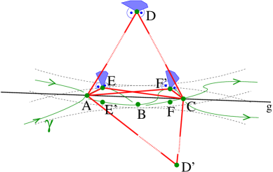
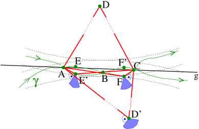
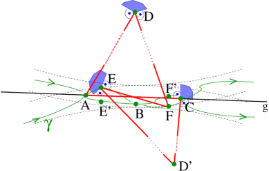
Figure 6.3: Three cases in the drawing plane $\nu_{\psi}^{\perp}$ discussed in the proof of Lemma 6.2. Intersecting the blue shaded regions leads to the angular region $J_{\psi}$ in each case.

If

$$\operatorname{dist}(E,g),\operatorname{dist}(F^{\prime},g)\geq\tfrac{\triangle[\gamma]}{2}\qquad\text{and}\qquad E,F^{\prime}\in G$$ (6.4)

then, using (6.2), the polygon $AECDAF^{\prime}CD^{\prime}A$ has three local maxima at $E$, $D$, and $F^{\prime}$ when projected onto any $\Phi(\vartheta,\psi)\in\mathbb{S}^{2}$ with $\left|\vartheta-\vartheta_{0}\right|\leq\arctan{\triangle[\gamma]}$. As $\arctan x\geq\tfrac{\pi}{4}x$ for $x\in[0,1]$, the set $J_{\psi}:=(\vartheta_{0}-\tfrac{\pi}{4}\triangle[\gamma],\vartheta_{0}+\tfrac{\pi}{4}\triangle[\gamma])$ is contained in $(\tfrac{\pi}{6},\tfrac{5\pi}{6})$ due to $\tfrac{\pi}{4}\triangle[\gamma]\stackrel{{\scriptstyle\text{\makebox[0.0pt][c]{\eqref{eq:zeta-thick}}}}}{{\leq}}\tfrac{\pi}{4}\zeta\leq\tfrac{1}{8\cdot 96}<0.0014$ and satisfies $\left|J_{\psi}\right|=\tfrac{\pi}{2}\triangle[\gamma]$.

Now assume that both $E$ and $F^{\prime}$ do not meet the (first) conditions in (6.4), so, by (6.3),

$$\operatorname{dist}(F,g),\operatorname{dist}(E^{\prime},g)\geq\tfrac{\triangle[\gamma]}{2}\qquad\text{and}\qquad E^{\prime},F\in G^{\prime}.$$

But this is symmetric to (6.4) since the polygon $AFCDAE^{\prime}CD^{\prime}A$ has three local minima at $E^{\prime}$, $D^{\prime}$, and $F$ when projected onto any $\Phi(\vartheta,\psi)\in\mathbb{S}^{2}$ with $\left|\vartheta-\vartheta_{0}\right|\leq\arctan\triangle[\gamma]$. Employing the same argument as for (6.4), this yields the desired as the number of local maxima and minima agrees.

Finally we have to deal with the “mixed case”. Without loss of generality we may assume

$$\operatorname{dist}(E,g),\operatorname{dist}(F,g)\geq\tfrac{\triangle[\gamma]}{2}\qquad\text{and}\qquad E\in G,F\in G^{\prime}.$$

But now the polygon $EFDACD^{\prime}E$ has three local maxima at $E$, $D$, and $C$ when projected onto any $\Phi(\vartheta,\psi)\in\mathbb{S}^{2}$ with $\left|\vartheta-\vartheta_{0}\right|\leq\arctan\triangle[\gamma]$ and $\left\langle\Phi(\vartheta,\psi),C-A\right\rangle>0$ which completes the proof with $\left|J_{\psi}\right|=\tfrac{\pi}{4}\triangle[\gamma]$. $\Box$

Proof 17 (Theorem 1.1).

Let us now assume that $\operatorname{tpc}_{\varphi}$, $\varphi\in(0,\pi]$, is the $C^{1}$-limit of $E_{\vartheta}$-minimizers  $\left(\gamma_{\vartheta}\right)_{\vartheta>0}$ as $\vartheta\to 0$. In the light of Proposition 5.4 for $a=2$, 6.1 and Lemma 6.2 we arrive at

$$C\vartheta^{2/3}\; \stackrel{{\scriptstyle\text{\makebox[0.0pt][c]{\eqref{eq:energy-growth-rate}}}}}{{\geq}}\;E_{\mathrm{bend}}(\gamma_{\vartheta})-(4\pi)^{2}=\int_{\mathbb{R}/\mathbb{Z}}\left|\gamma^{\prime\prime}_{\vartheta}\right|^{2}-(4\pi)^{2}\geq\left(\int_{\mathbb{R}/\mathbb{Z}}\left|\gamma^{\prime\prime}_{\vartheta}\right|\right)^{2}-(4\pi)^{2}$$

$$=\operatorname{TC}(\gamma_{\vartheta})^{2}-(4\pi)^{2}\geq 4\pi\left(\operatorname{TC}(\gamma_{\vartheta})-4\pi\right)=2\pi\int_{\mathbb{S}^{2}}\left(\mu\left(\gamma_{\vartheta},\nu\right)-2\right)\,\mathrm{d}A(\nu)$$

$$\geq 2\pi\operatorname{\mathscr{H}^{2}}\left(\mathcal{B}(\gamma_{\vartheta})\right)\geq\frac{\varphi\pi^{2}}{8\mathcal{R}(\gamma_{\vartheta})}\overset{\eqref{eq:ropelength-growth-rate}}{\geq}c\vartheta^{1/3}$$

for some positive constant $c$ depending on $\varphi$ and $\vartheta>0$ sufficiently small, which is a contradiction as $\vartheta\searrow 0$. Thus we have proven that the limit curve $\gamma_{0}\in\overline{\mathscr{C}_{\mathcal{T}({2,b})}}$ is isometric to the twice covered circle $\operatorname{tpc}_{0}$. $\Box$

Our Main Theorem now reads as follows.

Theorem 6.3 (Two bridge torus knot classes).

For any knot class $\mathcal{K}$ the following statements are equivalent.

1. $\mathcal{K}$ is the $(2,b)$-torus knot class for some odd integer $b\in\mathbb{Z}$ where $\left|b\right|\geq 3$;

2. $\inf_{\mathscr{C}(\mathcal{K})}E_{\mathrm{bend}}=(4\pi)^{2}$;

3. $\operatorname{tpc}_{\varphi}$ belongs to the $C^{1}$-closure of $\mathscr{C}(\mathcal{K})$ for some $\varphi\in[0,\pi]$ and $\mathcal{K}$ is not trivial;

4. for some $\varphi\in[0,\pi]$ the pair of tangentially intersecting circles $\operatorname{tpc}_{\varphi}$ is an elastic knot for $\mathscr{C}(\mathcal{K})$;

5. the unique elastic knot for $\mathscr{C}(\mathcal{K})$ is the twice covered circle $\operatorname{tpc}_{0}$.

Proof 18 (Theorem 6.3).

(i) $\Rightarrow$ (ii) follows from Theorem A.1 and the estimate in Lemma 5.1 for the comparison torus curves defined in (5.1).

(ii) $\Rightarrow$ (iii): As the bending energy of the circle amounts to $(2\pi)^{2}$, the knot class cannot be trivial. From Proposition 3.2 we infer that any elastic knot (which exists and belongs to the $C^{1}$-closure of $\mathscr{C}(\mathcal{K})$ according to Theorem 2.2) has constant curvature $4\pi$ a.e. Proposition 3.1 guarantees that any such elastic knot must have double points, which permits to apply Corollary 3.4. Thus, such an elastic knot coincides (up to isometry) with a tangential pair of circles $\operatorname{tpc}_{\varphi}$ for some $\varphi\in[0,\pi]$, which therefore lies in the $C^{1}$-closure of $\mathscr{C}(\mathcal{K})$ as desired.

(iii) $\Rightarrow$ (i) is an immediate consequence of Proposition 4.6 and Corollary 4.7.

Hence, so far we have shown the equivalence of the first three items.

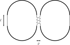
Figure 6.4: Explicit construction proving that $\operatorname{tpc}_{\varphi}$ is in the strong $C^{k}$-closure of $\mathscr{C}(\mathcal{K})$ for any $\varphi\in(0,\pi]$ and $k\in\mathbb{N}$.

(i) $\Rightarrow$ (v) is just the assertion of Theorem 1.1.

(v) $\Rightarrow$ (iv) is immediate.

(iv) $\Rightarrow$ (i): Since elastic knots for $\mathscr{C}(\mathcal{K})$ lie in the $C^{1}$-closure of $\mathscr{C}(\mathcal{K})$ by Theorem 2.2 we find by Proposition 4.6 for $\varphi\in(0,\pi]$, and by Corollary 4.7 for $\varphi=0$ that $\mathcal{K}=\mathcal{T}(2,b)$ for some odd $b\in\mathbb{Z}$, $\left|b\right|\geq 3$, or that $\mathcal{K}$ is trivial. The latter can be excluded since the unique elastic unknot is the once-covered circle by Proposition 3.1. $\Box$

Remark 6.4 (Strong $C^{k}$-closure).

Using an explicit construction like the one indicated in Figure 6.4 one can show as well that each item above is also equivalent to the following:

For every $\varphi\in[0,\pi]$ the corresponding tangential pair of circles $\operatorname{tpc}_{\varphi}$ belongs to the $C^{k}$-closure of $\mathscr{C}(\mathcal{K})$ for any $k\in\mathbb{N}$, and $\mathcal{K}$ is not trivial. $\Diamond$

Appendix A The Fáry–Milnor theorem for the $C^{1}$-closure of the knot class

Theorem A.1 (Extending the Fáry–Milnor theorem to the $C^{1}$-closure of $\mathcal{C}(\mathcal{K})$).

Let $\mathcal{K}$ be a non-trivial knot class and let $\gamma$ belong to the closure of $\mathscr{C}(\mathcal{K})$ with respect to the $C^{1}$-norm. Then the total curvature (5.2) satisfies

$$T(\gamma)\geq 4\pi.$$ (A.1)

We begin with two auxiliary tools and abbreviate, for any two vectors $X,Y\in\mathbb{R}^{3}$,

$$\overrightarrow{XY}:=Y-X.$$

Lemma A.2 (Approximating tangents).

Let $\left({\gamma}_{k}\right)_{k\in\mathbb{N}}\subset C^{1}(\mathbb{R}/\mathbb{Z},\mathbb{R}^{3})$ be a sequence of embedded arclength parametrized closed curves converging with respect to the $C^{1}$-norm to some limit curve $\gamma$. Assume that there are sequences $\left({x}_{k}\right)_{k\in\mathbb{N}},\left({y}_{k}\right)_{k\in\mathbb{N}}\subset[0,1)$ of parameters satisfying $x_{k}<y_{k}$ for all $k\in\mathbb{N}$ and $x_{k},y_{k}\to z\in[0,1)$ as $k\to\infty$. Then one has for $X_{k}:=\gamma_{k}(x_{k})$, $Y_{k}:=\gamma_{k}(y_{k})$

$$\frac{\overrightarrow{X_{k}Y_{k}}}{\left|X_{k}Y_{k}\right|}=\frac{Y_{k}-X_{k}}{|Y_{k}-X_{k}|}\xrightarrow{k\to\infty}\gamma^{\prime}(z)\in\mathbb{S}^{2}.$$ (A.2)

Proof 19.

Since all $\gamma_{k}$ are injective we find that $X_{k}\not=Y_{k}$ for $k\in\mathbb{N}$, so that the unit vectors $\frac{\overrightarrow{X_{k}Y_{k}}}{\left|X_{k}Y_{k}\right|}$ are well-defined, and a subsequence (still denoted by $\frac{\overrightarrow{X_{k}Y_{k}}}{\left|X_{k}Y_{k}\right|}$) converges to some limit unit vector $d\in\mathbb{S}^{2}$ because $\mathbb{S}^{2}$ is compact. It suffices to show that $d=\gamma^{\prime}(z)$ to conclude that the whole sequence converges to $\gamma^{\prime}(z),$ since any other subsequence of the $\frac{\overrightarrow{X_{k}Y_{k}}}{\left|X_{k}Y_{k}\right|}$ with limit $\tilde{d}\in\mathbb{S}^{2}$ satisfies $\tilde{d}=\gamma^{\prime}(z)$ as well.

We compute

$$\begin{split}&{\frac{\overrightarrow{X_{k}Y_{k}}}{\left|X_{k}Y_{k}\right|}-\frac{\gamma(y_{k})-\gamma(x_{k})}{y_{k}-x_{k}}}={\frac{\gamma_{k}(y_{k})-\gamma_{k}(x_{k})}{\left|\gamma_{k}(y_{k})-\gamma_{k}(x_{k})\right|}-\frac{\gamma(y_{k})-\gamma(x_{k})}{y_{k}-x_{k}}}\\ &=\frac{\int_{0}^{1}\gamma^{\prime}_{k}(x_{k}+\theta(y_{k}-x_{k}))\,\mathrm{d}\theta}{\left|\int_{0}^{1}\gamma^{\prime}_{k}(x_{k}+\theta(y_{k}-x_{k}))\,\mathrm{d}\theta\right|}-\int_{0}^{1}\gamma^{\prime}(x_{k}+\theta(y_{k}-x_{k}))\,\mathrm{d}\theta\\ &=\left(\frac{1}{\left|\int_{0}^{1}\gamma^{\prime}_{k}(x_{k}+\theta(y_{k}-x_{k}))\,\mathrm{d}\theta\right|}-1\right){\int_{0}^{1}\gamma^{\prime}_{k}(x_{k}+\theta(y_{k}-x_{k}))\,\mathrm{d}\theta}+{}\\ &\qquad{}+\int_{0}^{1}(\gamma^{\prime}_{k}-\gamma^{\prime})(x_{k}+\theta(y_{k}-x_{k}))\,\mathrm{d}\theta\\ &=\frac{1-\left|\int_{0}^{1}\gamma^{\prime}_{k}(x_{k}+\theta(y_{k}-x_{k}))\,\mathrm{d}\theta\right|}{\left|\int_{0}^{1}\gamma^{\prime}_{k}(x_{k}+\theta(y_{k}-x_{k}))\,\mathrm{d}\theta\right|}{\int_{0}^{1}\gamma^{\prime}_{k}(x_{k}+\theta(y_{k}-x_{k}))\,\mathrm{d}\theta}+{}\\ &\qquad{}+\int_{0}^{1}(\gamma^{\prime}_{k}-\gamma^{\prime})(x_{k}+\theta(y_{k}-x_{k}))\,\mathrm{d}\theta.\end{split}$$ (A.3)

From the assumptions we infer

$$1 \geq\left|\int_{0}^{1}\gamma^{\prime}_{k}(x_{k}+\theta(y_{k}-x_{k}))\,\mathrm{d}\theta\right|$$

$$\geq 1-2\|\gamma_{k}^{\prime}-\gamma^{\prime}\|_{L^{\infty}}-\left|\int_{0}^{1}(\gamma^{\prime}(x_{k}+\theta(y_{k}-x_{k}))-\gamma^{\prime}(x_{k}))\,\mathrm{d}\theta\right|$$

$$\geq 1-o(1)\quad\textnormal{as $k\to\infty$,}$$

so that in particular $\big{|}\int_{0}^{1}\gamma^{\prime}_{k}(x_{k}+\theta(y_{k}-x_{k}))\,\mathrm{d}\theta\big{|}\geq 1/2$ for $k\gg 1$. Inserting these two facts into (A.3) yields

$$\left|\frac{\overrightarrow{X_{k}Y_{k}}}{\left|X_{k}Y_{k}\right|}-\frac{\gamma(y_{k})-\gamma(x_{k})}{y_{k}-x_{k}}\right|\leq 2\left|1-\Big{|}\int_{0}^{1}\gamma^{\prime}_{k}(x_{k}+\theta(y_{k}-x_{k}))\,\mathrm{d}\theta\Big{|}\right|+\left\|\gamma^{\prime}_{k}-\gamma^{\prime}\right\|_{L^{{\infty}}}=o(1)$$

as $k\to\infty.$ $\Box$

Lemma A.3 (Regular curves cannot stop).

Let $\gamma\in C^{1}(\mathbb{R}/\mathbb{Z},\mathbb{R}^{3})$ be regular, i.e., $|\gamma^{\prime}|>0$ on $\mathbb{R}/\mathbb{Z}$, and let $0\leq x<y<1$ such that $\gamma(x)=\gamma(y)$. Then there is some $z\in(x,y)$ such that $\gamma(x)\neq\gamma(z)\neq\gamma(y)$.

Proof 20.

Assuming the contrary leads to a situation where $\gamma$ is constant on an interval of positive measure, i.e. $\gamma^{\prime}$ vanishes contradicting $\left|\gamma^{\prime}\right|>0$. $\Box$

Proof 21 (Theorem A.1).

Let $\left({\gamma}_{k}\right)_{k\in\mathbb{N}}$ be a sequence of knots in $\mathscr{C}(\mathcal{K})$ converging with respect to the $C^{1}$-norm to some limit curve $\gamma$. By Denne’s theorem [11, Main Theorem, p. 6], each knot $\gamma_{k}$, $k\in\mathbb{N}$, has an alternating quadrisecant, i.e., there are numbers $0\leq a_{k}<b_{k}<c_{k}<d_{k}<1$ such that the points $A_{k}:=\gamma_{k}(a_{k})$, $B_{k}:=\gamma_{k}(b_{k})$, $C_{k}:=\gamma_{k}(c_{k})$, $D_{k}:=\gamma_{k}(d_{k})$ are collinear and appear in the order $A$, $C$, $B$, $D$ on the quadrisecant line, see Figure A.1. (Note that our labeling of these points differs from that in [11].)

Figure A.1: An alternating quadrisecant

Without loss of generality we may assume $a_{k}\equiv 0$. By compactness, we may pass to a subsequence (without relabelling) such that $(a_{k},b_{k},c_{k},d_{k})$ converges to $(a,b,c,d)$ as $k\to\infty$. Of course,

$$0=a\leq b\leq c\leq d\leq 1.$$

Note that some or all of the corresponding points $A,B,C,D\in\mathbb{R}^{3}$, which are still collinear, may coincide and that $1\equiv 0$ in $\mathbb{R}/\mathbb{Z}$. By Milnor [24, Theorem 2.2] the total curvature of $\gamma$ is bounded from below by the total curvature of any inscribed (closed) polygon. For each possible location of the points $A,B,C,D$ we estimate the total curvature of $\gamma$ by means of suitably chosen inscribed polygons.

1. If $\left|BC\right|>0$ the polygon $ABCDA$ inscribed in $\gamma$ is non-degenerate in the sense that $0=a<b<c<d<1$. All exterior angles angles of $ABCDA$ equal $\pi$ and sum up to $4\pi$; hence (A.1) holds.

2. $\left|BC\right|=0$, i.e. $B=C$

   1. $\min\left(\left|AC\right|,\left|BD\right|\right)>0$

      1. If $b=c$, i.e. there is no loop of $\gamma$ between $B$ and $C$, we may consider the polygon $AB_{\varepsilon}C_{\varepsilon}DA$ with $B_{\varepsilon}:=\gamma(b-\varepsilon)$ and $C_{\varepsilon}:=\gamma(c+\varepsilon)$. Note that, in general, the point $B=C$ does not belong to the polygon, see Figure A.2. By arc-length parametrization, $B_{\varepsilon}$ and $C_{\varepsilon}$ cannot coincide for $0<\varepsilon\ll 1$.

         

         

         Figure A.2: (left) Situation 2.1.1, (right) Situation 2.1.2.

         We deduce that $\frac{\overrightarrow{B_{\varepsilon}C_{\varepsilon}}}{\left|B_{\varepsilon}C_{\varepsilon}\right|}$ converges to $\gamma^{\prime}(b)$ as $\varepsilon\to 0$. From Lemma A.2 we infer that $\gamma^{\prime}(b)$ points towards $A$ (due to $\frac{\overrightarrow{B_{k}A_{k}}}{\left|B_{k}A_{k}\right|}=\frac{\overrightarrow{B_{k}C_{k}}}{\left|B_{k}C_{k}\right|}\to\gamma^{\prime}(b)$ and the order $A_{k}C_{k}B_{k}D_{k}$ of the approximating points on the respective quadrisecant). Therefore, since $B_{\varepsilon}\to B$ and $C_{\varepsilon}\to C$ as $\varepsilon\to 0$, for given $\delta>0$ we obtain some $\varepsilon_{\delta}>0$ such that $\mathop{\mbox{$<\!\!\!)\,$}}\nolimits\left(\overrightarrow{AB_{\varepsilon}},\overrightarrow{B_{\varepsilon}C_{\varepsilon}}\right)>\pi-\delta$, $\mathop{\mbox{$<\!\!\!)\,$}}\nolimits\left(\overrightarrow{B_{\varepsilon}C_{\varepsilon}},\overrightarrow{C_{\varepsilon}D}\right)>\pi-\delta$, $\mathop{\mbox{$<\!\!\!)\,$}}\nolimits\left(\overrightarrow{C_{\varepsilon}D},\overrightarrow{DA}\right)>\pi-\delta$, and $\mathop{\mbox{$<\!\!\!)\,$}}\nolimits\left(\overrightarrow{DA},\overrightarrow{AB_{\varepsilon}}\right)>\pi-\delta$ for all $\varepsilon\in(0,\varepsilon_{\delta}]$. We arrive at a lower estimate of $4\pi-4\delta$ for the total curvature of the polygon $AB_{\varepsilon}C_{\varepsilon}DA$ which is a lower bound for the total curvature of $\gamma$. Letting $\delta\searrow 0$ yields the desired.

      2. If $b<c$ there is a loop of $\gamma$ between $B$ and $C$ according to Lemma A.3 such that we may choose some $m_{bc}\in(b,c)$ with $B=C\neq M_{BC}:=\gamma(m_{bc})$. The total curvature of $\gamma$ is bounded below by the total curvature of the polygon $ABM_{BC}CDA$. Let $\mu:=\mathop{\mbox{$<\!\!\!)\,$}}\nolimits\left(\overrightarrow{AB},\overrightarrow{BM_{BC}}\right)$. We obtain

         $$\mathop{\mbox{$<\!\!\!)\,$}}\nolimits\left(\overrightarrow{AB},\overrightarrow{BM_{BC}}\right) =\mu, \mathop{\mbox{$<\!\!\!)\,$}}\nolimits\left(\overrightarrow{BM_{BC}},\overrightarrow{M_{BC}C}\right) =\pi, \mathop{\mbox{$<\!\!\!)\,$}}\nolimits\left(\overrightarrow{M_{BC}C},\overrightarrow{CD}\right) =\pi-\mu,$$

         $$\mathop{\mbox{$<\!\!\!)\,$}}\nolimits\left(\overrightarrow{CD},\overrightarrow{DA}\right) =\pi, \mathop{\mbox{$<\!\!\!)\,$}}\nolimits\left(\overrightarrow{DA},\overrightarrow{AB}\right) =\pi.$$

   2. $\left|AC\right|=0$, $\left|BD\right|>0$, i.e. $A=B=C\neq D$

      1. The situation $a=b=c$ cannot occur as applying Lemma A.2 twice (and recalling the order $A_{k}C_{k}B_{k}D_{k}$ of the approximating points on the respective quadrisecant) yields $\gamma^{\prime}(b)=-\gamma^{\prime}(b)$ contradicting $\left|\gamma^{\prime}(b)\right|=1$.

      2. If $a=b<c$ we may simultaneously apply the techniques from 2.1.1 and 2.1.2 considering the polygon $A_{\varepsilon}BB_{\varepsilon}M_{BC}CDA_{\varepsilon}$ with $A_{\varepsilon}:=\gamma(a-\varepsilon)$ and $B_{\varepsilon}:=\gamma(b+\varepsilon)$. Note that, in contrast to 2.1.1, we inserted the point $B=C=A$ between $A_{\varepsilon}$ and $B_{\varepsilon}$ which is admissible due to $a-\varepsilon<a=b<b+\varepsilon$. We obtain the triangles $BB_{\varepsilon}M_{BC}$ and $CDA_{\varepsilon}$. We label the inner angles (starting from $B=C$ in each of the two triangles) by $\zeta_{\varepsilon}$, $\eta_{\varepsilon}$, $\theta_{\varepsilon}$ and $\lambda_{\varepsilon}$, $\mu_{\varepsilon}$, $\nu_{\varepsilon}$ and define

         $$\sigma_{\varepsilon} :=\mathop{\mbox{$<\!\!\!)\,$}}\nolimits\left(\overrightarrow{A_{\varepsilon}B},\overrightarrow{BB_{\varepsilon}}\right), \tau :=\mathop{\mbox{$<\!\!\!)\,$}}\nolimits\left(\overrightarrow{M_{BC}C},\overrightarrow{CD}\right),$$

         see Figure A.3.

         

         

         Figure A.3: (left) Situation 2.2.2. Note that, in general, the triangles $BB_{\varepsilon}M_{BC}$ and $CDA_{\varepsilon}$ are not coplanar and the angles $\sigma_{\varepsilon}$ and $\tau$ do not belong to any of the planes defined by the triangles. (right) Situations 2.2.4 and 2.4.3. For the latter one has to replace $D$ by $M_{DA}$.

         Therefore, the total curvature of the polygon amounts to the sum of exterior angles

         $$\sigma_{\varepsilon}+\left(\pi-\eta_{\varepsilon}\right)+\left(\pi-\theta_{\varepsilon}\right)+\tau+\left(\pi-\mu_{\varepsilon}\right)+\left(\pi-\nu_{\varepsilon}\right)=\sigma_{\varepsilon}+\tau+2\pi+\zeta_{\varepsilon}+\lambda_{\varepsilon}.$$

         Since $\frac{\overrightarrow{A_{\varepsilon}B}}{\left|A_{\varepsilon}B\right|}$ and $\frac{\overrightarrow{BB_{\varepsilon}}}{\left|BB_{\varepsilon}\right|}$ approximate $\gamma^{\prime}(b)$, which is a positive multiple of $\overrightarrow{CD}$ (because $c<d$ for $C\not=D$ which implies $\frac{\overrightarrow{C_{k}D_{k}}}{\left|C_{k}D_{k}\right|}=\frac{\overrightarrow{A_{k}C_{k}}}{\left|A_{k}C_{k}\right|}\to\gamma^{\prime}(b)=\frac{\overrightarrow{CD}}{\left|CD\right|}=\frac{\overrightarrow{BD}}{\left|BD\right|}$ by Lemma A.2), we deduce $\sigma_{\varepsilon}\to 0$, $\zeta_{\varepsilon}\to\pi-\tau$ and $\lambda_{\varepsilon}\nearrow\pi$ as $\varepsilon\searrow 0$ from Lemma A.2.

      3. For the case $a<b=c$ we consider the polygon $AM_{AB}B_{\varepsilon}CC_{\varepsilon}DA$ for $B_{\varepsilon}:=\gamma(b-\varepsilon)$ and $C_{\varepsilon}:=\gamma(c+\varepsilon)$ which may be treated similarly to 2.2.2.

      4. If $a<b<c$ we consider the polygon $AM_{AB}BM_{BC}CDA$ applying the technique from 2.1.2 twice. Defining

         $$\xi :=\mathop{\mbox{$<\!\!\!)\,$}}\nolimits\left(\overrightarrow{BM_{AB}},\overrightarrow{BM_{BC}}\right), \eta :=\mathop{\mbox{$<\!\!\!)\,$}}\nolimits\left(\overrightarrow{CM_{BC}},\overrightarrow{CD}\right), \zeta :=\mathop{\mbox{$<\!\!\!)\,$}}\nolimits\left(\overrightarrow{AD},\overrightarrow{AM_{AB}}\right)$$

         as indicated in Figure A.3 we arrive at

         $$\mathop{\mbox{$<\!\!\!)\,$}}\nolimits\left(\overrightarrow{AM_{AB}},\overrightarrow{M_{AB}B}\right) =\pi, \mathop{\mbox{$<\!\!\!)\,$}}\nolimits\left(\overrightarrow{M_{AB}B},\overrightarrow{BM_{BC}}\right) =\pi-\xi, \mathop{\mbox{$<\!\!\!)\,$}}\nolimits\left(\overrightarrow{BM_{BC}},\overrightarrow{M_{BC}C}\right) =\pi,$$

         $$\mathop{\mbox{$<\!\!\!)\,$}}\nolimits\left(\overrightarrow{M_{BC}C},\overrightarrow{CD}\right) =\pi-\eta, \mathop{\mbox{$<\!\!\!)\,$}}\nolimits\left(\overrightarrow{CD},\overrightarrow{DA}\right) =\pi, \mathop{\mbox{$<\!\!\!)\,$}}\nolimits\left(\overrightarrow{DA},\overrightarrow{AM_{AB}}\right) =\pi-\zeta$$

         so the total curvature of the polygon amounts to $6\pi-\xi-\eta-\zeta$. Consider the unit vectors $\frac{\overrightarrow{AM_{AB}}}{\left|AM_{AB}\right|}$, $\frac{\overrightarrow{AM_{BC}}}{\left|AM_{BC}\right|}$, and $\frac{\overrightarrow{AD}}{\left|AD\right|}$. Unless they are coplanar they define a unique triangle on $\mathbb{S}^{2}$ of area $<2\pi$ which is equal to the sum of the three angles between them, namely $\xi$, $\eta$, and $\zeta$. Therefore, we obtain the estimate $\xi+\eta+\zeta\leq 2\pi$.

   3. $\left|AC\right|>0$, $\left|BD\right|=0$, i.e. $A\neq B=C=D$. This case is symmetric to the preceding one.

   4. $\left|AC\right|=\left|BD\right|=0$, i.e. $A=B=C=D$. For $\Box_{1},\Box_{2},\Box_{3},\Box_{4}\in\left\{{=},{<}\right\}$ we abbreviate

      $$(\Box_{1},\Box_{2},\Box_{3},\Box_{4}):=\left(0\equiv a\Box_{1}b\Box_{2}c\Box_{3}d\Box_{4}1\equiv 0\right).$$

      Obviously there are $16$ cases.

      1. Impossible cases: as shown in 2.2.1, there cannot arise two neighboring equality signs. This excludes the following nine situations: $({=},{=},{=},{=})$, $({=},{=},{=},{<})$, $({=},{=},{<},{=})$, $({=},{=},{<},{<})$, $({=},{<},{=},{=})$, $({=},{<},{<},{=})$, $({<},{=},{=},{=})$, $({<},{=},{=},{<})$, $({<},{<},{=},{=})$.

      2. Two loops: for the situation $({=},{<},{=},{<})$ we consider the polygon

         $$A_{\varepsilon}BB_{\varepsilon}M_{BC}C_{\varepsilon}DD_{\varepsilon}M_{DA}A_{\varepsilon}$$

         with $A_{\varepsilon}:=\gamma(a-\varepsilon)$, $B_{\varepsilon}:=\gamma(b+\varepsilon)$, $C_{\varepsilon}:=\gamma(c-\varepsilon)$, and $D_{\varepsilon}:=\gamma(d+\varepsilon)$. We obtain the (in general non-planar) quadrilaterals $BB_{\varepsilon}M_{BC}C_{\varepsilon}$ and $DD_{\varepsilon}M_{DA}A_{\varepsilon}$. Proceeding similarly to 2.2.2, we label the inner angles (starting from $B$) by $\zeta_{\varepsilon}$, $\eta_{\varepsilon}$, $\theta_{\varepsilon}$, $\iota_{\varepsilon}$ and $\lambda_{\varepsilon}$, $\mu_{\varepsilon}$, $\nu_{\varepsilon}$, $\xi_{\varepsilon}$ and define

         $$\sigma_{\varepsilon} :=\mathop{\mbox{$<\!\!\!)\,$}}\nolimits\left(\overrightarrow{A_{\varepsilon}B},\overrightarrow{BB_{\varepsilon}}\right), \tau_{\varepsilon} :=\mathop{\mbox{$<\!\!\!)\,$}}\nolimits\left(\overrightarrow{C_{\varepsilon}D},\overrightarrow{DD_{\varepsilon}}\right),$$

         see Figure A.4.

         

         

         Figure A.4: (left) Situation 2.4.2. Note that both quadrilaterals $BB_{\varepsilon}M_{BC}C_{\varepsilon}$ and $DD_{\varepsilon}M_{DA}A_{\varepsilon}$ are, in general, non-planar. (right) Situation 2.4.4.

         For the angular sum in a non-planar quadrilateral we obtain

         $$\zeta_{\varepsilon}+\eta_{\varepsilon}+\theta_{\varepsilon}+\iota_{\varepsilon} \leq 2\pi \lambda_{\varepsilon}+\mu_{\varepsilon}+\nu_{\varepsilon}+\xi_{\varepsilon}\leq 2\pi.$$

         The total curvature of the polygon amounts to the sum of exterior angles

         $$\sigma_{\varepsilon}+\left(\pi-\eta_{\varepsilon}\right)+\left(\pi-\theta_{\varepsilon}\right)+\left(\pi-\iota_{\varepsilon}\right)+\tau_{\varepsilon}+\left(\pi-\mu_{\varepsilon}\right)+\left(\pi-\nu_{\varepsilon}\right)+\left(\pi-\xi_{\varepsilon}\right)$$

         $$\geq\sigma_{\varepsilon}+\tau_{\varepsilon}+2\pi+\zeta_{\varepsilon}+\lambda_{\varepsilon}.$$

         From Lemma A.2 we infer $\zeta_{\varepsilon},\lambda_{\varepsilon}\nearrow\pi$. The case $({<},{=},{<},{=})$ is shifted by one position.

      3. Three loops: the case $({<},{<},{<},{=})$ leads to the polygon

         $$AM_{AB}BM_{BC}CM_{CD}D$$

         which is treated similarly to 2.2.4; here $\overrightarrow{CM_{CD}}$ plays the rôle of $\overrightarrow{CD}$ in 2.2.4. The shifted cases $({=},{<},{<},{<})$, $({<},{=},{<},{<})$, $({<},{<},{=},{<})$ are symmetric.

      4. Four loops: As 2.4.3 in fact works for $({<},{<},{<},{\leq})$ it also covers the situation $({<},{<},{<},{<})$. Alternatively we consider the polygon

         $$AM_{AB}BM_{BC}CM_{CD}DM_{DA}A$$

         as drawn in Figure A.4 with

         $$\mathop{\mbox{$<\!\!\!)\,$}}\nolimits\left(\overrightarrow{AM_{AB}},\overrightarrow{M_{AB}B}\right)=\mathop{\mbox{$<\!\!\!)\,$}}\nolimits\left(\overrightarrow{BM_{BC}},\overrightarrow{M_{BC}C}\right)=\mathop{\mbox{$<\!\!\!)\,$}}\nolimits\left(\overrightarrow{CM_{CD}},\overrightarrow{M_{CD}D}\right)$$

         $$=\mathop{\mbox{$<\!\!\!)\,$}}\nolimits\left(\overrightarrow{DM_{DA}},\overrightarrow{M_{DA}A}\right)=\pi.$$

$\Box$

References

- [1] Emil Artin. Theorie der Zöpfe. Abh. Math. Sem. Univ. Hamburg, 4(1):47–72, 1925.
- [2] Sergey Avvakumov and Alexey Sossinsky. On the normal form of knots. Russ. J. Math. Phys., 21(4):421–429, 2014.
- [3] Simon Blatt. Note on continuously differentiable isotopies. Report 34, Institute for Mathematics, RWTH Aachen, August 2009.
- [4] Simon Blatt and Philipp Reiter. Stationary points of O’Hara’s knot energies. Manuscripta Math., 140(1-2):29–50, 2013.
- [5] Simon Blatt and Philipp Reiter. How nice are critical knots? Regularity theory for knot energies. J. Phys.: Conf. Ser., 544:012020, 2014.
- [6] Simon Blatt and Philipp Reiter. Modeling repulsive forces on fibres via knot energies. Mol. Based Math. Biol., 2:56–72, 2014.
- [7] Simon Blatt, Philipp Reiter, and Armin Schikorra. Hard analysis meets critical knots (Stationary points of the Moebius energy are smooth). Accepted by Transactions of the AMS, 2012.
- [8] Gregory Buck and Eric J. Rawdon. Role of flexibility in entanglement. Phys. Rev. E, 70:011803, Jul 2004.
- [9] Gerhard Burde and Heiner Zieschang. Knots, volume 5 of de Gruyter Studies in Mathematics. Walter de Gruyter & Co., Berlin, second edition, 2003.
- [10] Richard H. Crowell and Ralph H. Fox. Introduction to knot theory. Springer-Verlag, New York-Heidelberg, 1977. Reprint of the 1963 original, Graduate Texts in Mathematics, No. 57.
- [11] Elizabeth Denne. Alternating Quadrisecants of Knots. ArXiv Mathematics e-prints, October 2005.
- [12] Yuanan Diao, Claus Ernst, and E. J. Janse van Rensburg. Thicknesses of knots. Math. Proc. Cambridge Philos. Soc., 126(2):293–310, 1999.
- [13] István Fáry. Sur la courbure totale d’une courbe gauche faisant un nœud. Bull. Soc. Math. France, 77:128–138, 1949.
- [14] Werner Fenchel. Geschlossene Raumkurven mit vorgeschriebenem Tangentenbild. Jahresbericht der Deutschen Mathematiker-Vereinigung, 39:183–185, 1930.
- [15] Riccardo Gallotti and Olivier Pierre-Louis. Stiff knots. Phys. Rev. E (3), 75(3):031801, 14, 2007.
- [16] Oscar Gonzalez and John H. Maddocks. Global curvature, thickness, and the ideal shapes of knots. Proc. Natl. Acad. Sci. USA, 96(9):4769–4773 (electronic), 1999.
- [17] Oscar Gonzalez, John H. Maddocks, Friedemann Schuricht, and Heiko von der Mosel. Global curvature and self-contact of nonlinearly elastic curves and rods. Calc. Var. Partial Differential Equations, 14(1):29–68, 2002.
- [18] Zheng-Xu He. The Euler-Lagrange equation and heat flow for the Möbius energy. Comm. Pure Appl. Math., 53(4):399–431, 2000.
- [19] Richard Koch and Christoph Engelhardt. Closed space curves of constant curvature consisting of arcs of circular helices. J. Geom. Graph., 2(1):17–31, 1998.
- [20] Joel Langer and David A. Singer. Curve straightening and a minimax argument for closed elastic curves. Topology, 24(1):75–88, 1985.
- [21] Chun-Chi Lin and Hartmut R. Schwetlick. On a flow to untangle elastic knots. Calc. Var. Partial Differential Equations, 39(3-4):621–647, 2010.
- [22] Richard A. Litherland, Jonathan K. Simon, Oguz C. Durumeric, and Eric J. Rawdon. Thickness of knots. Topology Appl., 91(3):233–244, 1999.
- [23] Jenelle Marie McAtee Ganatra. Knots of constant curvature. J. Knot Theory Ramifications, 16(4):461–470, 2007.
- [24] John W. Milnor. On the total curvature of knots. Ann. of Math. (2), 52:248–257, 1950.
- [25] Jun O’Hara. Energy of a knot. Topology, 30(2):241–247, 1991.
- [26] Philipp Reiter. All curves in a -neighbourhood of a given embedded curve are isotopic. Report 4, Institute for Mathematics, RWTH Aachen, October 2005.
- [27] Philipp Reiter. Regularity theory for the Möbius energy. Commun. Pure Appl. Anal., 9(5):1463–1471, 2010.
- [28] Philipp Reiter. Repulsive knot energies and pseudodifferential calculus for O’Hara’s knot energy family , . Math. Nachr., 285(7):889–913, 2012.
- [29] Dale Rolfsen. Knots and links. Publish or Perish, Inc., Berkeley, Calif., 1976. Mathematics Lecture Series, No. 7.
- [30] Friedemann Schuricht and Heiko von der Mosel. Euler-Lagrange equations for nonlinearly elastic rods with self-contact. Arch. Ration. Mech. Anal., 168(1):35–82, 2003.
- [31] Friedemann Schuricht and Heiko von der Mosel. Global curvature for rectifiable loops. Math. Z., 243(1):37–77, 2003.
- [32] Paweł Strzelecki and Heiko von der Mosel. On rectifiable curves with -bounds on global curvature: self-avoidance, regularity, and minimizing knots. Math. Z., 257(1):107–130, 2007.
- [33] Paweł Strzelecki and Heiko von der Mosel. Menger curvature as a knot energy. Physics Reports, 530:257–290, 2013.
- [34] Paweł Strzelecki and Heiko von der Mosel. How averaged menger curvatures control regularity and topology of curves and surfaces. In Knotted, Linked and Tangled Flux in Quantum and Classical Systems, Journal of Physics Conference Series. IoP, Cambridge, 2014.
- [35] De Witt Sumners. DNA, knots and tangles. In The mathematics of knots, volume 1 of Contrib. Math. Comput. Sci., pages 327–353. Springer, Heidelberg, 2011.
- [36] Heiko von der Mosel. Minimizing the elastic energy of knots. Asymptot. Anal., 18(1-2):49–65, 1998.
- [37] Heiko von der Mosel. Elastic knots in Euclidean -space. Ann. Inst. H. Poincaré Anal. Non Linéaire, 16(2):137–166, 1999.