Temporal Behavior of Rabi Oscillation in Nanomechanical QED System with a Nonlinear Resonator

Abstract

In nanomechanical QED system, consisting of a charge qubit and a nanomechanical resonator with intrinsic nonlinearity, we study the temporal behavior of Rabi oscillation in the nonlinear Jaynes-Cummings model. Using microscopic master equation approach, we solve time evolution of the density operator describing this model. Also, the probability of excited state of charge qubit is calculated. These analytic calculations show how nonlinearity parameter and decay rates of two different excited states of the qubit-resonator system affect time-oscillating and decaying of Rabi oscillation.

I Introduction

Actually, any quantum system interacting with the environment (the bath) can not be isolated from the environment completely. Zurek (1983) In quantum information and quantum computation, DiVincenzo (2000) the decay process of quantum system induced by quantum fluctuations of the bath is very important for the qubit. In quantum optics, Scully (1997) the Jaynes-Cummings model has been one of the most important models, Jaynes (1963) which describes the light-matter interaction of a two-level atom and a single mode of the quantized electromagnetic field. Raimond (2001) Among these light-matter interaction issues, Cohen (1998) the revivals and collapses of the atomic population inversion (also named Rabi oscillation) has been studied in the literatures. Eberly (1980, 1981); Rempe (1987)

Decay of Rabi oscillation has also been used as a tool to characterize the decoherence in superconducting qubits (charge qubit, phase qubit and flux qubit). Makhlin (2001); Nori (2005) Recently, in circuit QED system, Blais (2004) the researchers have performed spectroscopic measurements of a superconducting qubit dispersively coupled to a nonlinear resonator driven by a pump microwave field. Ong (2011) Also in nanomechanical QED system, the integration of Josephson junction qubit and nanomechanical resonators are attracting considerable attentions. Gao (2009); Xue (2007); Roukes (2009, 2013) The dynamics of all these qubit-resonator systems could be described by the Jaynes-Cummings Hamiltonian.

When intrinsic nonlinearity of nanomechanical resonator Hartmann (2014) is considered in the coupled qubit-resonator system, superconducting qubit can be used to probe quantum fluctuations of nonlinear resonator. Blais (2013) And the nonlinearity can be used to create nonclassical states in mechanical systems Paris (2015); Hartmann (2015) and selectively address the nanomechanical qubit transitions in quantum information processing. Hartmann (2013)

In previous studies, Camichael (1993) master equation approach has been used to deal with the issues in open quantum system. In this paper, considering the influence of the environment on this nanomechanical QED system, we can use microscopic master equation approach Scala (2007) to solve time evolution of the density operator for the qubit-resonator system and study the temporal Behavior of Rabi Oscillation.

The paper is structured as follows. In sec.II, a nonlinear Jaynes-Cummings Model P Gora (1992) is used to describe the dynamics of the coupled qubit-nanomechanical resonator system. In sec.III, using microscopic master equation approach, we solve time evolution of density operator for the qubit-resonator system. The probability on excited state of the qubit is calculated to show the temporal process of Rabi oscillation. Finally, the results are summarized.

II the qubit-resonator system

In nanomechanical QED system, we can use a Jaynes-Cummings type Hamiltonian to describes the dynamics of the qubit-resonator system consisting of a charge qubit and a nanomechanical resonator system,

$$H_{JC}=\frac{\omega_{q}}{2}\sigma_{z}+g\left(a\sigma_{+}+a^{\dagger}\sigma_{-}\right)+\omega_{c}a^{\dagger}a.$$ (1)

Considering the nonlinearity of nanomechanical resonator, the Hamiltonian for this qubit-resonator system writes Gao (2013)

$$H_{S}=H_{JC}+\chi a^{\dagger}a+\chi\left(a^{\dagger}a\right)^{2}.$$ (2)

Here the rotating-wave approximation ($\omega_{q}=\omega_{a}=\omega$) and $\hbar=1$ is adopted. Corresponding to charge qubit and nanomechanical resonator, the lowering (raising) operator $\sigma_{-}$ ($\sigma_{+}$) and the annihilation (creation) operator $a$ ($a^{\dagger}$) satisfy the commutation relation $[\sigma_{-},\sigma_{+}]=\sigma_{z}$ and $[a,a^{\dagger}]=1$. The Hamiltonian in Eq. (2) describes the dynamics of a nonlinear Jaynes-Cummings model, P Gora (1992) and a quartic potential $x^{4}$ Hartmann (2014) gives nonlinear part $\chi\left(a^{\dagger}a\right)^{2}$ which leads to the phonon-phonon interaction in nanomechanical QED systems. The $g$ is the coupling constant and the $\chi$ is the nonlinearity parameter ($\chi\ll g$).

Solving the Hamiltonian $H_{S}$, we get the ground state $|E_{0}\rangle=|00\rangle$ with energy $E_{0}=-\omega/2$ and excited state doublets

$$\left|E_{1+}\right\rangle = \cos\left(\frac{\theta}{2}\right)\left|10\right\rangle+\sin\left(\frac{\theta}{2}\right)\left|01\right\rangle,$$

$$\left|E_{1-}\right\rangle = -\sin\left(\frac{\theta}{2}\right)\left|10\right\rangle+\cos\left(\frac{\theta}{2}\right)\left|01\right\rangle,$$

for $n=1,2,3,...$ with energy

$$E_{1\pm}=\left(\frac{\omega}{2}+\chi\right)\pm\Omega.$$

Some parameters are defined, i.e., $\Omega=\sqrt{g^{2}+\chi^{2}}$ and $\theta=\arcsin\left(g/\Omega\right)$.

With the loss of nanomechanical resonator, the total Hamiltonian

$$H_{\text{total}}=H_{S}+H_{I}+H_{B}$$

consists of three parts, i.e., the system part $H_{S}$, the interaction part

$$H_{I}=\sum_{j}\xi_{j}\left(ab_{j}^{\dagger}+a^{\dagger}b_{j}\right)$$

and the bath part

$$H_{B}=\sum_{j}\omega_{j}b_{j}^{\dagger}b_{j}.$$

Where $b_{j}$ and $b_{j}^{\dagger}$ are bosonic annihilation and creation operators for the bath oscillators for the mode frequency $\omega_{j}$ ($j=1,2,...$).

In this paper, we adopt microscopic master equation approach Scala (2007) to solve time evolution of density operator ($\rho$) for the qubit-resonator system, our master equation is

$$\dot{\rho}=\mathcal{L}\rho$$ (3)

where $\mathcal{L}$ is a time-independent linear superoperator.

Using the microscopic master equation approach, Scala (2007) we obtain the eigen-equations

$$\mathcal{L}\rho_{k}=\lambda_{k}\rho_{k}.$$ (4)

The $\left\{\rho_{k}\right\}$ is a set of eigenoperators due to the superoperator $\mathcal{L}$ with the eigenvalue $\left\{\lambda_{k}\right\}$ for the index $k$.

Given initial state of the qubit-resonator system, the initial reduced density operator $\rho\left(0\right)$ is expanded in terms of $\rho_{k}$,

$$\rho\left(0\right)=\sum_{k}C_{k}\rho_{k}$$ (5)

where the $C_{k}$s are time-independent coefficients. The results in Ref.Scala (2007) tell us that time evolution of reduced density operator $\rho$ will be

$$\rho\left(t\right)=\sum_{k}C_{k}e^{{}_{\lambda_{k}t}}\rho_{k}.$$ (6)

Now only one excitation is interested, our truncated basis $\left\{|E_{1+}\rangle,|E_{1-}\rangle,|E_{0}\rangle\right\}$ consists of the three lowest eigenstates due to the Hamiltonian $H_{S}$,

Now we can rewrite the master equation in Eq. (3),

$$\dot{\rho}=-i\left[H_{S},\rho\right]+\mathcal{L}_{+}\rho+\mathcal{L}_{-}\rho.$$ (7)

Here the non-unitary parts of dissipative dynamics are described by $\mathcal{L}_{+}\rho$ and $\mathcal{L}_{-}\rho$,

$$\mathcal{L_{\pm}\rho} = \frac{\gamma_{\pm}}{2}\left|E_{0}\right\rangle\left\langle E_{1\pm}\right|\rho\left|E_{1\pm}\right\rangle\left\langle E_{0}\right|$$

$$-\frac{\gamma_{\pm}}{4}\left(\left|E_{1\pm}\right\rangle\left\langle E_{1\pm}\right|\rho+\rho\left|E_{1\pm}\right\rangle\left\langle E_{1\pm}\right|\right).$$

The superoperator $\mathcal{L}_{\pm}$describe the transitions between the higher excited state $|E_{\pm}\rangle$ and the ground state $|E_{0}\rangle$ induced by the environment. The corresponding decay rate $\gamma_{+}$ ($\gamma_{-}$) describes the transition from the excited state $|E_{1+}\rangle$ ($|E_{1-}\rangle$) to the ground state $|E_{0}\rangle$, these transitions are induced by the interaction between the system and the environment.

With respect to the system Hamiltonian $H_{S}$ in Eq. (2), the eigenoperators $\rho_{k}$s are obtained,

$$\rho_{1} = \left|E_{0}\right\rangle\left\langle E_{0}\right|,$$

$$\rho_{2} = \left|E_{1,-}\right\rangle\left\langle E_{1,-}\right|-\left|E_{0}\right\rangle\left\langle E_{0}\right|,$$

$$\rho_{3} = \left|E_{1,+}\right\rangle\left\langle E_{1,+}\right|-\left|E_{0}\right\rangle\left\langle E_{0}\right|,$$

$$\rho_{4} = \left|E_{0}\right\rangle\left\langle E_{1,-}\right|,$$

$$\rho_{5} = \left|E_{0}\right\rangle\left\langle E_{1,+}\right|,$$

$$\rho_{6} = \left|E_{1,-}\right\rangle\left\langle E_{1,+}\right|,$$

$$\rho_{7} = \rho_{4}^{\dagger},\ \rho_{8}=\rho_{5}^{\dagger},\ \rho_{9}=\rho_{6}^{\dagger}.$$

The corresponding eigenvalues $\lambda_{k}$s (for $k=1,2,3,...,9$) are

$$\lambda_{1} = 0,\ \lambda_{2}=-\frac{\gamma_{1-}}{2},\ \lambda_{3}=-\frac{\gamma_{1+}}{2},$$

$$\lambda_{4} = i\left(\omega+\chi-\Omega\right)-\frac{1}{4}\gamma_{1-},$$

$$\lambda_{5} = i\left(\omega+\chi+\Omega\right)-\frac{1}{4}\gamma_{1+},$$

$$\lambda_{6} = i(2\Omega)-\frac{1}{4}\left(\gamma_{1+}+\gamma_{1-}\right),$$

and

$$\lambda_{7}=\lambda_{4}^{*},\ \lambda_{8}=\lambda_{5}^{*},\ \lambda_{9}=\lambda_{6}^{*}.$$

III Rabi Oscillation

In traditional cavity QED theory, Raimond (2001) the Rabi oscillation means that there exists energy exchange of one photon between a two-level atom and a single mode quantized field in cavity. Considering the nonlinearity of nanomechanical resonator, we study the decay process of Rabi oscillation in the nonlinear Jaynes-Cummings model described by the Hamiltonian in Eq. (2).

Given the initial state of the qubit-resonator system $|\psi\left(0\right)\rangle=|e\rangle\otimes|0\rangle$, it means that the qubit is in excited state $|e\rangle$ and the resonator is in vacuum state $|0\rangle$. Thus, the initial reduced density operator reads

$$\rho\left(0\right)=\left|\psi\left(0\right)\right\rangle\left\langle\psi\left(0\right)\right|.$$

Expanding $\rho\left(0\right)$ into some eigenoperators $\rho_{k}$s, we obtain a set of coefficients $C_{k}$s,

$$C_{1}=1,\ C_{2}=\frac{1}{2}\left(1-\cos\theta\right),\ C_{3}=\frac{1}{2}\left(1+\cos\theta\right),$$

$$C_{6}=C_{9}=-\frac{1}{2}\sin\theta,$$

and

$$C_{4}=C_{5}=C_{7}=C_{8}=0.$$

According to Eq.(6), the time evolution of density operator for the qubit-resonator system is calculated as

$$\rho\left(t\right) = C_{1}e^{{}_{\lambda_{1}t}}\rho_{1}+C_{2}e^{{}_{\lambda_{2}t}}\rho_{2}$$

$$+C_{3}e^{{}_{\lambda_{3}t}}\rho_{3}+C_{6}e^{{}_{\lambda_{6}t}}\rho_{6}+C_{9}e^{{}_{\lambda_{9}t}}\rho_{9}.$$

Here the probability of the qubit in the excited (upper) state $\left|e\right\rangle$ is

$$P_{e}(t) = \left\langle e0\right|\rho\left(t\right)\left|e0\right\rangle$$ (8)

$$= \left[\frac{1}{2}\left(1-\cos\theta\right)e^{-\frac{\gamma_{1-}}{4}t}-\frac{1}{2}\left(1+\cos\theta\right)e^{-\frac{\gamma_{1+}}{4}t}\right]^{2}$$

$$+\sin^{2}\theta e^{-\frac{\gamma_{1+}+\gamma_{1-}}{4}t}\cos^{2}\left(\Omega t\right).$$

It characterizes the temporal behavior of Rabi oscillation in the qubit-resonator system, decay process of Rabi oscillation owns the periodic structure of time oscillating.

The nanomechanical resonator is assumed to be an ideal resonator ($\chi=0$), and ignoring the difference of decay rates ($\gamma_{1+}=\gamma_{1-}=\gamma$), then the probability $P_{e}(t)$ becomes

$$P_{e}(t)=e^{-\frac{\gamma}{2}t}\cos^{2}\left(gt\right).$$ (9)

It describes the well known Rabi oscillation in Jaynes-Cummings model.Jaynes (1963) Comparing the results in Eq. (8) with Eq. (9), we find that nonlinearity parameter $\chi$ and decay rates $\gamma_{1+}\neq\gamma_{1-}$ modify the periodic structure of time oscillating in Rabi oscillation.

To further clarify the dependence of nonlinearity parameter and decay rates on the probability $P_{e}(t)$ clearly, some figures are plotted with parameters $\omega=1.0,\ g=0.1$. Here, we take the frequency $\omega$ as the unit for all these parameters.

In Fig.$\,1$, the probability $P_{e}(t)$ versus time $t$ is plotted with parameters $\chi=0$ and $\gamma_{1+}=\gamma_{1-}=0.004$. Figure 1 shows the well known Rabi oscillation, it verifies the results in Eq. (9).

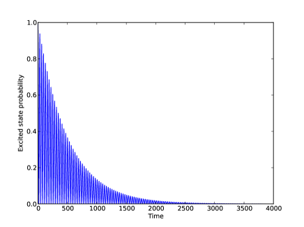
Figure 1: Rabi oscillation in Jaynes-Cummings model. Some parameters are $\chi=0$ and $\gamma=0.004$.

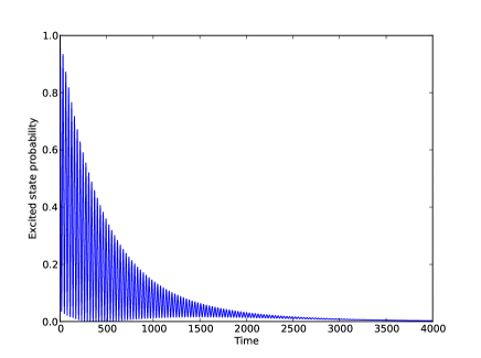
Figure 2: The probability $P_{e}\left(t\right)$ vs the time $t$, where the excite states ($|1+\rangle$ and $|1-\rangle$) own the different decay rate ($\gamma_{1-}=0.001$ and $\gamma_{1+}=0.007$) and $\chi=0$.04.

In Fig.$\,2$, the probability $P_{e}(t)$ versus time $t$ is plotted with parameters $\chi=0.04$, $\gamma_{1+}=0.007$ and $\gamma_{1-}=0.001$. Figure 2 shows that nonlinearity parameter $\chi$ and decay rates ($\gamma_{1+}\neq\gamma_{1-}$) modify the periodic structure of time oscillating in Rabi oscillation, which is obviously different from Figure 1.

Based on those results in Eq. (8,9), we find that nonlinearity parameter $\chi$ slows down the time-oscillating period of Rabi oscillation $T=\left(2\Omega\right)^{-1}$. In the following, we will study how nonlinearity parameter $\chi$ and decay rates ($\gamma_{1+}\neq\gamma_{1-}$) affect the temporal behavior in Rabi oscillation solely.

Firstly, assuming the same decay rates $\gamma_{1-}=\gamma_{1+}=\gamma$ and nonlinearity parameter $\chi\neq 0$, the probability in Eq. (8) becomes

$$P_{e}(t)=e^{-\frac{\gamma}{2}t}\left(\cos^{2}\theta+\sin^{2}\theta\cos^{2}\left(\Omega t\right)\right).$$ (10)

The dependence of the probability $P_{e}(t)$ on nonlinearity parameter $\chi$ is plotted in Fig.$\,3$. When $\cos^{2}\left(\Omega t\right)=0$, the minimum of the probability

$$P_{e}(t)=e^{-\frac{\gamma}{2}t}\cos^{2}\theta$$ (11)

decays exponentially, which is different from the well known Rabi oscillation in Fig.$\,1$.

Secondly, assuming no nonlinearity $\chi=0$ and different decay rates ($\gamma_{1+}\neq\gamma_{1-}$), the probability in Eq. (8) becomes

$$P_{e}(t)=\frac{1}{4}\left(e^{-\frac{\gamma_{1-}}{4}t}-e^{-\frac{\gamma_{1+}}{4}t}\right)^{2}+e^{-\frac{\gamma_{1+}+\gamma_{1-}}{4}t}\cos^{2}\left(gt\right).$$

The dependence of the probability $P_{e}(t)$ on different decay rates is plotted in Fig.$\,4$. When $\cos^{2}\left(gt\right)=0$, the minimum of the probability

$$P_{e}(t)=\frac{1}{4}\left(e^{-\frac{\gamma_{1-}}{4}t}-e^{-\frac{\gamma_{1+}}{4}t}\right)^{2}$$

shows that the difference of decay rates between $\gamma_{1-}$ and $\gamma_{1+}$ does not affect the short-time behavior and long-time behavior of Rabi oscillation obviously, which is seen in Fig.$\,4$.

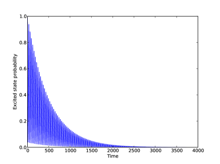
Figure 3: The probability $P_{e}\left(t\right)$ vs the time $t$, where the excite states ($|1+\rangle$ and $|1-\rangle$) own the same decay rate ($\gamma_{1+}=\gamma_{1-}=\gamma=0.004$) and nonlinearity parameter $\chi=0.04$.

Figure 4: The probability $P_{e}\left(t\right)$ vs the time $t$, the excite states ($|1+\rangle$ and $|1-\rangle$) of the qubit-resonator system own the different decay rate ($\gamma_{1-}=0.001$ and $\gamma_{1+}=0.007$) and nonlinearity parameter $\chi=0$.

Analytically, we can study the short-time behavior of Rabi oscillation, then the probability $P_{e}\left(t\right)$ becomes

$$P_{e}(t)=\exp\left\{-\left[\cos\theta\left(\frac{\gamma_{1+}}{4}-\frac{\gamma_{1-}}{4}\right)+\frac{\gamma_{1-}+\gamma_{1+}}{4}\right]t\right\}.$$ (12)

Ignoring the nonlinearity of nanomechanical resonator or the difference of decay rates, i.e., $\chi=0$ or $\gamma_{1-}=\gamma_{1+}$, the probability $P_{e}\left(t\right)$ becomes

$$P_{e}(t)=\exp\left\{-\frac{\gamma_{1-}+\gamma_{1+}}{4}t\right\}.$$ (13)

According to the results in Eq. (12) and Eq. (13), we find that both nonlinearity parameter $\chi$ and the difference of decay rates ($\gamma_{1+}\neq\gamma_{1-}$) affect dominate the short-time behavior of Rabi oscillation jointly. Also, these two factors speed up the decay of Rabi oscillation in short-time limit.

IV conclusions

In summary, we have studied the dynamics of the nanomechanical QED system consisting of a charge qubit and a nanomechanical resonator. The temporal behavior of Rabi oscillations is analytically studied while the intrinsic nonlinearity of nanomechanical resonator is considered. With the loss of nanomechanical resonator, microscopic master equation approach is used to calculate the excited-state probability of charge qubit in this nonlinear Jaynes-Cummings model. These results show that nonlinearity parameter and decay rates can affect time-oscillating and decaying of Rabi oscillation solely or jointly.