Generation of three-dimensional entanglement between two spatially separated atoms via shortcuts to adiabatic passage
Jing-bo Lin
Department of Physics, College of Science, Yanbian
University, Yanji, Jilin 133002, People’s Republic of China
Yan Liang
Department of Physics, College of Science, Yanbian
University, Yanji, Jilin 133002, People’s Republic of China
Xin Ji 111E-mail: jixin@ybu.edu.cnDepartment of Physics, College of Science, Yanbian University, Yanji, Jilin
133002, People’s Republic of China
Shou Zhang
Department of Physics, College of Science, Yanbian University, Yanji, Jilin
133002, People’s Republic of China
Abstract
Abstract
We propose a scheme for generating three-dimensional entanglement
between two atoms trapped in two spatially separated cavities
reapectively via shortcuts to adiabatic passage based on the
approach of Lewis-Riesenfeld invariants in cavity quantum
electronic dynamics. By combining Lewis-Riesenfeld invariants with
quantum Zeno dynamics, we can generate three dimensional
entanglement of the two atoms with high fidelity. The Numerical
simulation results show that the scheme is robust against the
decoherences caused by the photon leakage and atomic spontaneous
emission.
1. Introduction
Quantum entanglement plays a significant role not only in testing
quantum nonlocality, but also in a variety of quantum information
tasks
AKE ; CHB ; CHBS ; CHBG ; KMH ; MHVB ; SBZGCG ; GV ; SHT1997 ; MI2000 ; CD2000 ; JWDD1996 .
Recently, high-dimensional entanglement is becoming more and more
important since they are more secure than qubit systems,
especially in the aspect of quantum key distribution. Besides, it
has been demonstrated that violations of local realism by two
entangled high-dimensional systems are stronger than that by
two-dimensional systems DPMW2000 . So a lot of works have
been done theoretically and experimentally in generating
high-dimensional entanglement
WG2011 ; LP2012 ; WCYC2013 ; QCW2013 ; XQ201405 ; XQ201402 ; SL2014 ; YLS2015 ; AAGA2001 ; AGA2002 .
In order to realize the entanglement generation or population
transfer in a quantum system with time-dependent interacting
field, many schemes have been put forward. Such as pulses,
composite pulses, rapid adiabatic passage(RAP), stimulated Raman
adiabatic passage , and their variants
KHB1998 ; PIMS2007 ; NVTB2001 . STIRAP is widely used in
time-dependent interacting field because of the robustness for
variations in the experimental parameters. But it usually requires
a relatively long interaction time, so that the decoherence would
destroy the intended dynamics, and finally lead to an error
result. Therefore, reducing the time of dynamics towards the
perfect final outcome is necessary and perhaps the most effective
method to essentially fight against the dissipation which comes
from noise or losses accumulated during the operational processes.
Rencently, various schemes have been explored theoretically and
experimentally to construct shortcuts for adiabatic passage
XASA2010 ; KPYR2011 ; JXPP2011 ; ARXD2012 ; AFTS2012 ; AC2013 ; MYLJ2014 ; YHC2014 ; YLQ2015 ; YLC2015 ; YLX2015 .
Unfortunately, as far as we know, the research of constructing
shortcuts to adiabatic passage for generating entanglement has not
been comprehensively studied.
In this paper, we construct an effective shortcuts to adiabatic
passage for generating three dimentional entanglement between two
atoms trapped in two spatially separated cavities connected by a
fiber based on the Lewis-Riesenfeld invariants and quantum Zeno
dynamics (QZD). The time for generating three dimentional
entanglement in our scheme is much shorter time than that based on
adiabatic passage technique. Moreover, the strict numerical
simulations demonstrate that our scheme is insensitive to the
decoherence caused by spontaneous emission and photon leakage.
This paper is structured as follows: In Section 2, we give a brief
description about Lewis-Riesenfeld invariants and QZD. In Section
3, we construct a shortcuts for generating three dimentional
entanglement. Section 4 shows the numerical simulation results and
feasibility analysis. The conclusion appears in Section 5.
2. Preliminary theory
2.1. Lewis-Riesenfeld invariants
We first give a brief description about Lewis-Riesenfeld
invariants theory HRL1969 ; MAL2009 . A quantum system is
governed by a time-dependent Hamiltonian , and the
corresponding time-dependent Hermitian invariant satisfies
(1)
The solution of the time-dependent Schrödinger equation
can be expressed by a superposition of
invariant dynamical modes
(2)
where is time-independent amplitude, is the
Lewis-Riesenfeld phase, is one of the
orthogonal eigenvectors of the invariant , satisfying
, with
being real constant. And the Lewis-Riesenfeld phases
are defined as
(3)
2.2. Quantum Zeno dynamics
Quantum Zeno effect is an interesting phenomenon in quantum
mechanics. Recent studies PVGS2000 ; PS2002 ; PGS2009 show that
a quantum Zeno evolution will evolve away from its initial state,
but it remains in the Zeno subspace defined by the measurements
PVGS2000 via frequently projecting onto a multidimensional
subspace. This is known as QZD. We consider a system which is
governed by the Hamiltonian
(4)
where is the Hamiltonian of the investigated quantum
system and the is the interaction Hamiltonian
performing the measurement. is a coupling constant, and when
it satisfies , the whole system is governed
by the evolution operator
(5)
where is one of the eigenprojections of with
eigenvalues ().
3. Shortcuts to adiabatic passage for generating
three-dimensional entanglement of two atoms
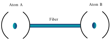
Figure 1: The schematic
setup for generating two atoms three-dimensional entanglement. The
two atoms are trapped in two spatially separated optical cavities
connected by a fiber.
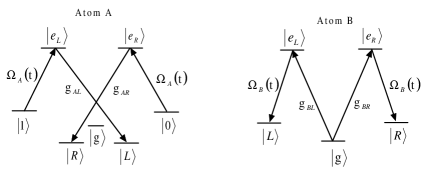
Figure 2: The level
configurations of atom A and B.
The schematic setup for generating three-dimensional entanglement
of two atoms is shown in Fig.1. We consider a
cavity-fibre-cavity system, in which two atoms are trapped in the
corresponding optical cavities connected by a fiber. Under the
short fiber limit , only the resonant mode of
the fiber will interact with the cavity mode SMB2006 , where
is the length of the fiber and is the decay rate of the
cavity field into a continuum of fiber modes. The corresponding
level structures of atoms are shown in Fig. 2. Atom A has
two excited states , and five ground
states , , , and
, while atom B is a five-level system with three ground
states , and , two excited
states and . For atom A, the
transitions and
are driven by classical
fields with the same Rabi frequency . And the
transitions and
are resonantly driven by
the corresponding cavity mode with -circular
polarization and the coupling strength is . For
atom B, the transitions
and are driven by
classical fields with the same Rabi frequency , and
the transitions and
are resonantly driven by
the corresponding cavity mode with -circular
polarization and the coupling strength is . The
whole Hamiltonian in the interaction picture can be written as
():
(6)
(7)
(9)
where is the coupling strength between cavity mode and the
fiber mode, is the annihilation operator for the fiber
mode with -circular polarization, is the
annihilation operator for the corresponding cavity field with
-circular polarization, and is the coupling
strength between the corresponding cavity mode and the trapped
atom.
In order to obtain the following two atoms three-dimensional
entanglement:
(10)
we assume atom A in the state
(11)
while atom B in the state , both the cavity modes and
the fiber mode in vacuum state
. Then we present how to
realize the evolutions of the atom state
to , to
, to
.
For the initial state
,
the whole system evolves in the subspace spanned by
(12)
Seting ,
then both the condition and the Zeno condition can
be satisfied ( and
correspond respectively to and in Eq.
(4)). By performing the unitary transformation
under condition , the
Hilbert subspace can be divided into five invariant Zeno subspaces
PS2002 ; PGS2009 :
(13)
with the eigenvalues , , ,
, and
, where we assume
for simplicity. Here
(14)
and the corresponding projection
(15)
Under the above condition, the system Hamiltonian can be rewritten
as the following form PGS2009 :
(17)
When we choose the initial state ,
the Hamiltonian reduces to
(18)
where and
.
In order to construct the shortcuts for generating
three-dimensional entanglement by the dynamics of invariant based
inverse engineering, we need to find out the Hermitian invariant
operator , which satisfies
. Since possesses SU(2)
dynamical symmetry, can be easily given by
MA2001 ; XCE2011
(19)
where is an arbitrary constant with units of frequency to
keep with dimensions of energy, and are
time-dependent auxiliary parameters which satisfy the equations
(20)
Then we can derive the expressions of and
easily as follows:
(21)
The solution of Shrödinger equation
with respect to the instantaneous
eigenstates of can be written as
,
where is the Lewis-Riesenfeld phase in Eq.
(3), , and
is the eigenstate of the invariant
(23)
In order to transfer the population from state to
, we choose the parameters as
(24)
where is a time-independent small value and is
the total pulse duration. After the precise calculation, we can
easily obtain
(25)
and
(26)
When ,
(28)
where ( are
the Lewis-Riesenfeld phases). We choose
, then
.
On the other hand, for the initial state ,
the whole system evolves in the subspace spanned by
(29)
The effective Hamiltonian in the subspace is
(30)
where
.
With the same way as above, we can realize the transition from
to .
Then we make one qubit operation on atom A to make
become with the help of laser pulses resonant
with A atomic transition
and
with the
corresponding Rabi frequencies and
. In this step, the Hamiltonian in the interaction
picture can be written as ()
(31)
With the same method as above, we can choose
(32)
Here we choose , and with the similar processes as above
we can realize the transformation from to
.
Up to now, the initial state
(33)
of the whole system has evolved into the state
(34)
Ignoring the global phase, the two atoms are in three-dimensional
entanglement, with the cavity-modes and the fiber mode in vacuum
state.
4. Numerical simulations and feasibility analysis
In the following, we present the numerical validation of the
mechanism proposed for the generation of three-dimensional
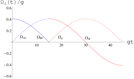
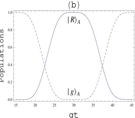
entanglement of the two atoms. Fig. 3 shows the
time-dependence laser pulse as a function of
for a fixed value , and . With
these parameters the Zeno condition can be met well. The
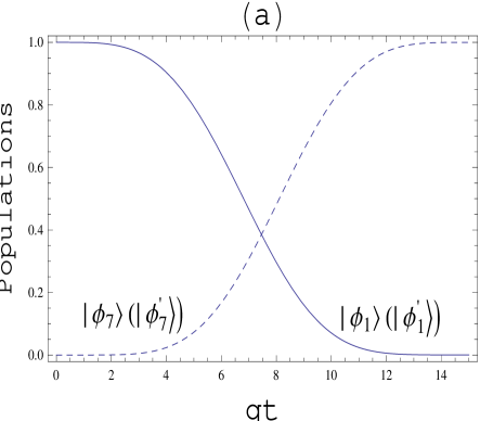
populations of states and
swap perfectly when
, as shown in Fig. 4(a), and the populations of
states and also swap perfectly
when as shown in Fig. 4(b).
Figure 3: Temporal
profile of the time dependence Rabi frequencies
versus with (dash blue line),
(solid blue line), (dash red
line), (solid red line).
Figure 4: (a) Time evolutions of the populations of the
corresponding system states with the initial states
. (b) Time evolutions of the
populations with the initial state . The system
parameters are set to be ,
with .
Figure 5: The effect of
atomic spontaneous emission on the fidelity of the
three-dimensional entanglement with different values of the photon
leakage rates of cavities or fiber.
In addition, whether a scheme is available largely depends on the
robustness to the loss and decoherence. so we consider the effects
of loss and decoherence on the entanglement generation. The
corresponding master equation for the whole system density matrix
has the following form:
(38)
where . is the photon leakage rate
of th fiber mode, is the photon leakage rate
of -circular polarization mode in th cavity,
is th atomic spontaneous emission rate
of cavity from the excited state to the
corresponding ground state .
,
and . For simplicity, we assume
,
. The initial condition . Fig. 5 shows
the fidelity as a function of
the dimensional parameter with different values of
by numerically solving the master equation (38).
From Fig. 5 we can see that, the fidelity for
three-dimensional entanglement is higher than when
and . It shows that our scheme is robust
against decoherence caused by photon leakage of cavities and
fiber, and atomic spontaneous emission.
Now we give a brief analysis of the feasibility in experiment of
our scheme. The appropriate atomic level configuration can be
obtained from the hyperfine structure of cold alkali-metal atoms
TWS2007 ; BWH2009 ; MLM2011 . Here we adopt the Cs.
5S1/2 ground level
corresponds to and
corresponds to
, respectively, while 5P3/2 excited
level corresponds to
. Other hyperfine levels in the
ground-state manifold can be used as for atom A. For
atom B, the states and
correspond to and
of 5S1/2 ground levels, respectively. And
corresponds to
of 5P3/2 excited level.
5. Conclusion
In conclusion, we have proposed a scheme for generating
three-dimensional entanglement of two spatially separated atoms
through the shortcut to adiabatic passage and QZD. We also study
the influences of system parameters, such as photon leakage of
cavities and fiber, and atomic spontaneous emission, on the
fidelity through numerical simulation. The numerical simulation
results show that our scheme is very robust against the system
parameters.
Acknowledgment
This work was supported by the National Natural Science Foundation
of China under Grant Nos. 11464046 and 61465013.
References
(1) A. K. Ekert, “Quantum cryptography based on Bell s theorem,” Phys. Rev. Lett. 67, 661-663 (1991).
(2) C. H. Bennett, F. Bessette, G. Brassard, L. Salvail, and J. Smolin, “Experimental quantum cryptography,” Journal
of Cryptology 5, 3-28 (1992).
(3) C. H. Bennett and S. J. Wiesner, “Communication via one- and two-particle operators on Einstein-Podolsky-Rosen states,” Phys. Rev. Lett. 69,
2881-2884 (1992).
(4) C. H. Bennett, G. Brassard, C. Crpeau, R. Jozsa, A. Peres, and W. K. Wootters, “Teleporting an unknown quantum state via dual classical and Einstein-Podolsky-Rosen channels,” Phys. Rev. Lett. 70, 1895-1899 (1993).
(5) K. Mattle, H. Weinfurter, P. G. Kwiat, and A. Zeilinger, “Dense coding in experimental quantum communication,” Phys. Rev. Lett. 76, 4656-4659 (1996).
(6) M. Hillery, V. Bužek, and A. Berthiaume, “Quantum secret sharing,” Phys. Rev. A 59, 1829-1834 (1999).
(7) S. B. Zheng and G. C. Guo, “Efficient scheme for two-atom entanglement and quantum information processing in cavity QED,” Phys. Rev. Lett. 85, 2392-2395 (2000).
(8) G. Vidal, “Efficient classical simulation of slightly entangled quantum computations,” Phys. Rev. Lett. 91, 147902 (2003).
(9) H. K. Lo, S. Popescu, and T. Spiller, Introduction to Quantum Computation and Information (World Scientific, Singapore, 1997).
(10) M. A. Nielsen and I. L. Chuang, Quantum Computation and Quantum Information (Cambridge University Press, Cambridge, 2000).
(11) C. H. Bennett and D. P. DiVincenzo, “Quantum information and computation,” Nature (London) 404, 247-255 (2000).
(12) J. J. Bollinger, W. M. Itano, D. J. Wineland, and D. J. Heinzen, “Optimal frequency measurements with maximally correlated states,” Phys. Rev. A 54, R4649-R4652 (1996).
(13) D. Kaszlikowski, P. Gnacinski, M. Żukowski, W. Miklaszewski, and A. Zeilinger, “Violations of local realism by two entangled
N-Dimensional systems are stronger than for two qubits,” Phys.
Rev. Lett. 85, 4418-4421 (2000).
(14) W. A. Li and G. Y. Huang, “Deterministic generation of a three-dimensional entangled state via quantum Zeno dynamics,” Phys. Rev. A 83, 022322 (2011).
(15) L. B. Chen, P. Shi, C. H. Zheng, and Y. J. Gu, “Generation of three-dimensional entangled state between a single
atom and a Bose-Einstein condensate via adiabatic passage,” Opt.
Express 20, 14547-14555 (2012).
(16) X. Wu, Z. H. Chen, M. Y. Ye, Y. H. Chen, and X. M. Lin, “Generation of multiparticle three-dimensional entanglement state via adiabatic passage,” Chin. Phys. B
22, 040309 (2013).
(17) Q. C. Wu and X. Ji, “Generation of steady three- and four-dimensional entangled states via quantum-jump-based feedback,” Quantum Inf. Process. 12, 3167-3178 (2013).
(18) X. Q. Shao, J. B. You, T. Y. Zheng, C. H. Oh, and S. Zhang, “Stationary three-dimensional entanglement via dissipative Rydberg pumping,” Phys. Rev. A 89, 052313 (2014).
(19) X. Q. Shao, T. Y. Zheng, C. H. Oh, and S. Zhang, “Dissipative creation of three-dimensional entangled state in optical cavity via spontaneous emission,” Phys. Rev. A 89, 012319 (2014).
(20) S. L. Su, X. Q. Shao, H. F. Wang, and S. Zhang, “Preparation of three-dimensional entanglement for distant atoms in coupled cavities via atomic spontaneous emission and cavity decay,” Sci. Rep. 4, 7566 (2014).
(21) Y. Liang, S. L. Su, Q.C. Wu, X. Ji, and S. Zhang, “Adiabatic passage for three-dimensional entanglement generation through quantum Zeno dynamics,” Opt. Express 23(4), 5064-5077 (2015).
(22) A. Mair, A. Vaziri, G. Weihs, and A. Zeilinger, “Entanglement of the orbital angular momentum states of photons,” Nature (London) 412,
313-316 (2001).
(23) A. Vaziri, G. Weihs, and A. Zeilinger, “Experimental two-photon, three-dimensional entanglement for quantum communication,” Phys. Rev. Lett. 89, 240401 (2002).
(24) K. Bergmann, H. Theuer, and B. W. Shore, “Coherent population transfer among quantum states
of atoms and molecules,” Rev. Mod. Phys. 70, 1003-1025
(1998).
(25) P. Král, I. Thanopulos, and M. Shapiro, “Colloquium: Coherently controlled adiabatic passage,” Rev. Mod. Phys. 79, 53-77 (2007).
(26) N. V. Vitanov, T. Halfmann, B. W. Shore, and K. Bergmann, “Laser-induced populstion transfer by adiabatic passage techniques,” Annu. Rev. Phys. Chem. 52, 763-809 (2001).
(27) X. Chen, A. Ruschhaupt, S. Schmidt, A. del Campo, D. Guéry-Odelin, and J. G. Muga, “Fast optimal frictionless
atom cooling in harmonic traps: Shortcut to adiabaticity,” Phys.
Rev. Lett. 104, 063002 (2010).
(28) K. H. Hoffmann, P. Salamon, Y. Rezek, and R. Kosloff, “Time-optimal controls for frictionless cooling in harmonic traps,” Europhys. Lett. 96, 60015 (2011).
(29) J. F. Schaff, X. L. Song, P. Capuzzi, P. Vignolo, and G. Labeyrie, “Shortcut to adiabaticity for an interacting Bose-Einstein condensate,” Europhys. Lett. 93, 23001 (2011).
(30) A. Ruschhaupt, X. Chen, D. Alonso, and J. G. Muga, “Optimally robust shortcuts to population inversion in two-level quantum systems,” New Journal of Physics, 14, 093040 (2012).
(31) A. Walther, F. Ziesel, T. Ruster, S. T. Dawkins, K. Ott, M. Hettrich, K. Singer, F. Schmidt-Kaler, and U. Poschinger,
“Controlling fast transport of cold trapped ions,” Phys. Rev.
Lett. 109, 080501 (2012).
(32) A. del Campo, “Shortcuts to adiabaticity by counter-adiabatic driving,” Phys. Rev. Lett. 111, 100502 (2013).
(33) M. Lu, Y. Xia, L. T. Shen, J. Song, and N. B. An, “Shortcuts to adiabatic passage for population transfer and maximum entanglement creation between two atoms in a cavity,” Phys. Rev. A 89, 012326 (2014).
(34) Y. H. Chen, Y. Xia, Q. Q. Chen, and J. Song, “Efficient shortcuts to adiabatic passage for fast population transfer in multiparticle systems,” Phys. Rev. A 89, 033856 (2014).
(35) Y. Liang, Q. C. Wu, S. L. Su, X. Ji, and S. Zhang, “Shortcuts to adiabatic passage for multiqubit controlled-phase gate,” 91, 032304 (2015).
(36) Y. Liang, C. Song, X. Ji, and S. Zhang, “Fast CNOT gate between two spatially separated atoms via shortcuts to adiabatic passage,” Opt. Express 23(18), 23798-23810 (2015).
(37) Y. Liang, X. Ji, H. F. Wang, and S. Zhang, “Deterministic SWAP gate using shortcuts to adiabatic passage,” 12, 115201 (2015).
(38) H. R. Lewis and W. B. Riesenfeld, “ An exact quantum theory of the time-dependent harmonic oscillator and of a charged particle in a time-dependent
electromagnetic field,” J. Math. Phys. 10, 1458 (1969).
(39) M. A. Lohe, “Exact time dependence of solutions to the time-dependent Schr?odinger equation,” J. Phys. A: Math. and Theor. 42, 035307 (2009).
(40) P. Facchi, V. Gorini, G. Marmo, S. Pascazio, and E. C. G.
Sudarshan, “Quantum Zeno dynamics,” Phys. Lett. A 275,
12-19 (2000).
(41) P. Facchi and S. Pascazio, “Quantum Zeno Subspaces,” Phys. Rev. Lett. 89, 080401 (2002).
(42) P. Facchi, G. Marmo, and S. Pascazio, “Quantum Zeno dynamics and quantum Zeno subspaces,” J. Phys: Conf. Ser. 196,
012017 (2009).
(43) A. Serafini, S. Mancini, and S. Bose, “Distributed quantum computation via optical fibers,” Phys. Rev. Lett. 96(1),
010503 (2006).
(44) A. Mostafazadeh, Dynamical Invariants, Adiabatic Approximation, and the Geometric Phase
(Nova Science Pub Incorporated 2001).
(45) X. Chen, E. Torrontegui, and J. G. Muga, “Lewis-Riesenfeld invariants and transitionless quantum driving,” Phys. Rev. A 83, 062116 (2011).
(46) T. Wilk, S. C. Webster, A. Kuhn, and G. Rempe,
“Single-atom single-photon quantum interface,” Science,
317, 488-490 (2007).
(47) B. Weber, H. P. Specht, T. Müller, J.
Bochmann, M. Mücke, D. L. Moehring, and G. Rempe,
“Photon-photon entanglement with a single trapped atom,” Phys.
Rew. Lett. 102, 030501(2009).
(48) M. Lettner, M. Mücke, S. Riedl, C. Hahn, S.
Baur, J. Bochmann, S. Ritter, S. Dürr, and G. Rempe, “Remote
entanglement between a single atom and a Bose-Einstein
condensate,” Phys. Rew. Lett. 106, 210503 (2011).