Structure in the 3D Galaxy Distribution: III. Fourier Transforming the Universe: Phase and Power Spectra

Abstract

We demonstrate the effectiveness of a relatively straightforward analysis of the complex 3D Fourier transform of galaxy coordinates derived from redshift surveys. Numerical demonstrations of this approach are carried out on a volume-limited sample of the Sloan Digital Sky Survey redshift survey. The direct unbinned transform yields a complex 3D data cube quite similar to that from the Fast Fourier Transform (FFT) of finely binned galaxy positions. In both cases deconvolution of the sampling window function yields estimates of the true transform. Simple power spectrum estimates from these transforms are roughly consistent with those using more elaborate methods. The complex Fourier transform characterizes spatial distributional properties beyond the power spectrum in a manner different from (and we argue is more easily interpreted than) the conventional multi-point hierarchy. We identify some threads of modern large scale inference methodology that will presumably yield detections in new wider and deeper surveys.

1 Introduction: Perspective and Assumptions

This paper takes the background established by two previous publications on the multiscale structure of the Universe (Way et al., 2011, 2015, Papers I and II, respectively) in a different direction: direct 3D Fourier analysis of the galaxy positions. The goal is to maximize three things: simplicity, extraction of information from the data, and independence from assumptions and models. The following list describes the principles underlying this work. These items are largely methodological clarifications and not cosmological assumptions as such. In many cases our approach differs from previous work, references to which are deferred to the next section.

1. A Limited Cosmological Sample. Testing models against finite-volume data usually involves consideration of cosmic variance. To avoid the need to postulate properties of unobserved data that is inherent in this notion, we here adopt a viewpoint nicely described (but not necessarily endorsed) by Peebles (1975a):

   “One can adopt the view that we have only one Universe, that we can see only part of it, and that the analysis ought to be based on that part alone.”

   See Section 5.2 for an approach to cosmic variance using resampling techniques.

2. Nearly Noise-free Data. For our purposes the uncertainty due to observational errors in the SDSS data is essentially negligible (Section 5). We thus do not follow the common practice of treating irregularities at small scales as noise (or as not “topologically persistent”) with smoothing or other practices that destroy information. Structure detected on all scales carries significant information about the Universe.

3. Point Distribution, not a Continuous Field. Galaxies are often assumed to trace some underlying continuous field – e.g. an averaged luminous or dark matter density, or a probability density for the presence of a galaxy. We address the spatial distribution of galaxies without reference to any continuous field, and treat galaxies as discrete entities whose spatial distribution carries information about the structure of the Universe. This approach is consistent with equal treatment of all galaxies – i.e. massive galaxies are not given more weight than light ones.

4. Summary Distributions. There are two qualitatively different approaches:

   • detailed representation and interpretation of local structures

   • estimation of a few summary, global distributional parameters

   again nicely spelled out in Peebles (1975a). In Papers I and II we opted for the former. Here we derive several Fourier analysis functionals with the goal of estimating important global parameters.

5. Gaussianity. We approach the search for signs of non-Gaussianity via the Fourier phase spectrum. A complete characterization of Gaussianity is contained in the power spectrum. The information about non-Gaussianity contained in the phase spectrum is organized in a form that is relatively easy to interpret (cf. Section 4.2).

6. Absolute Clustering. Most previous analysis has treated spatial correlations as departures from the mean density (e.g. Yu & Peebles, 1969; Landy and Szalay, 1993). In contrast density estimates here and in Papers I and II are absolute. In fact as discussed in Section 3.2 subtraction of a reference value, such as the mean, does not make sense for a direct Fourier transform as in Eq. (4). In addition our approach avoids some technical problems (Jones, Martinez, Saar and Trimble, 2004).

7. Explicit Deconvolution of the 3D Selection Function. Using standard Fourier transform methods we avoid constructs such as Monte Carlo simulations of “un-clustered” points within the selected volume. For example, Feldman, Kaiser and Peacock (1994) state: “Our approach is to take the Fourier transform of the real galaxies minus the transform of a synthetic catalog with the same angular and radial selection function as the real galaxies but otherwise without structure.” Perhaps this approach has meaning in the context of a model based on underlying randomness, but is not a prescription for deconvolving the selection function. Further, in consonance with item 1 and 2, we avoid interpreting such variance as a measure of uncertainty. While various deconvolution methods have been employed for both CMB and galaxy data, we believe the direct 3D Fourier deconvolution described in Section 3.5 is novel.

8. Use All the Data. In order to maximize the information gleaned from the analysis, where possible we use all of the data. For example we do not discard galaxies near the edges of the data space in order to simplify the shape of the window function (Section 3.3), but the next item indicates one case where we feel a cut on the data is justified.

9. Volume-Limited Samples. Throughout, as in Papers I and II, we use well defined volume-limited samples. This minor violation of the previous item is made for the good reason that it avoids bias corrections necessary for a magnitude-limited sample.

10. Omitted Effects. Due to the small radial depth of our relatively shallow volume limited sample (redshift $\leq 0.12$) and our interest in the simplest analysis, we have neglected many processes known to affect the data, including evolution and nonlinear cosmological terms, peculiar velocities, gravitational lensing, and local and non local GR terms depending on Bardeen potentials and their temporal derivatives (Raccanelli et al., 2015, especially Fig. 1).

The few of these viewpoints that are nonstandard are not meant as criticisms of other approaches. The goal here is limited to investigating the simplest possible way to extract spatial frequency information, largely avoiding model-specific assumptions and concentrating more on the phase spectrum and less on the power spectrum.

The organization of the rest of this paper is as follows: Following a brief survey of prior work in Section 2, Section 3 provides explicit details of two different ways to compute Fourier transforms – a direct unbinned approach and a fast Fourier transform of galaxy coordinates in 3D spatial bins – and a simple procedure for deconvolution of the sampling window from the estimated galaxy transform. Section 4 gives examples of application of the complex 3D Fourier transform, briefly dwelling on the amplitude (power) spectrum but focusing on the phase spectrum as a measure of Gaussianity. Section 5 briefly addresses uncertainties. The epilog in Section 6 provides a summary and pointers to three statistical techniques the should be useful in future research. Two appendices provide a check of the analysis and some MatLab code.

2 Previous Work

A small part of the earlier relevant literature can be found in Limber (1953); Gunn (1965); Yu & Peebles (1969); Peebles (1975a); Peebles and Hauser (1973, 1974b). The cosmological importance of power spectrum analysis has recently been extensively discussed in Carron, Wolk and Szapudi (2015), especially in the context of galaxy redshift surveys (e.g. Vogeley and Szalay, 1996, Sec. 1.1). Fourier phases have been studied in connection with cosmic microwave background data (see e.g. Chiang et al., 2003; Naselsky, Doroshkevich and Verkhodanov, 2003, 2004; Chiang, Naselsky and Coles, 2004; Naselsky, Chiang, Olesen and Novikov, 2005; Chiang and Naselsky, 2007; Kovács, Szapudi and Frei, 2013; Ferreira and Magueijo, 1997). More recently phase analysis is beginning to be applied to galaxy redshift data (Hikage et al., 2005; Matsubara, 2007; Wolstenhulme, Bonvin and Obreschkow, 2015; Eggemeier et al., 2015).

Some relevant work on non-Gaussianity, much in the context of CMB but with application to large scale – or more appropriately multi-scale – structure includes: Hikage et al. (2006) who provide a general overview, Sefusatti and Komatsu (2007) who discuss the bi-spectrum for high redshift galaxies, Hikage et al. (2008) who discuss the application of Minkowski functionals, Sánchez and Cole (2008) who estimate the power spectrum using Fourier methods based on work by Feldman, Kaiser and Peacock (1994), Martínez-González (2009) and Lentati, Hobson and Alexander (2014) for pulsar timing studies, and also Kovács, Szapudi and Frei (2013). See Coles et al. (2005) for application of Fourier methods to the 2dF galaxy redshift survey, employing the Fourier based method of Percival, Verde and Peacock (2004), a generalization of the minimum variance method of Feldman, Kaiser and Peacock (1994). Coles et al. (2005) derive power spectra and compare them to several empirical (e.g. Tegmark et al., 2004a) and theoretical results. See Kitaura (2012) for derivation of some statistics relevant to non-Gaussianity in galaxy clustering. Other work on non-Gaussianity can be found in (Coles and Chiang, 2000; Rocha et al, 2001; Watts, Coles and Melott, 2003; Tegmark et al., 2004b).

Efstathiou and Moody (2001) describe a method of recovering the three-dimensional power spectrum from measurements of the angular correlation function applied to the APM galaxy survey – one of the first large surveys using automatic plate measuring methods. See also Querre, Starck and Martínez (2002) for discussion of the galaxy distribution using multiscale methods in general, and 3D implementations of the á trous algorithm, and the ridgelet and beamlet transforms in particular. Percival, Verde & Peacock (2004, hereafter PVP) studied luminosity-dependent galaxy clustering with spherically averaged Fourier analysis. Coles et al. (2005) applied the Fourier based method of PVP to the 2dF galaxy redshift survey. This approach in turn is a generalization of the minimum variance method of Feldman, Kaiser and Peacock (1994). See recent papers (Slepian and Eisenstein, 2015a, b, c; Doré et al., 2015) for estimation of three-point correlation functions and their application to problems in dark matter cosmology. Alam, Ata, Bailey et al. (2016) give a recent summary of relevant literature and extensive analysis of data from the SDSS-III Baryon Oscillation Spectroscopic Survey.

3 3D Fourier Transforms

The sub-sections below describe the procedures used to compute the complex Fourier transform of the galaxy distribution – first reviewing the data and then outlining direct and binned transforms of the galaxy positions and the corresponding data window, concluding with a Fourier-based procedure to deconvolve the effect of this window function.

3.1 The Data

Below we Fourier analyze the SDSS DR7 data described in Papers I and II, namely the NASA/Ames Research Center SDSS Value Added Galaxy Catalog (AMES-VAGC). Data Release 7 of the SDSS was augmented using the New York University Value Added Catalog (see Appendix A of Paper II for details and references). As a reminder, redshift $\zeta$, right ascension $\alpha$ and declination $\delta$ were converted to rectangular Cartesian coordinates with the formulas

$$x=\zeta cos(\delta)cos(\alpha)$$

$$y=\zeta cos(\delta)sin(\alpha)$$ (1)

$$z=\zeta sin(\delta)$$

and no cosmological corrections were made in view of the low-redshift nature of the sample. The one small difference is that, since the analysis here does not involve Voronoi tessellation, the omission of the small sample of galaxies near the edges of the data space (Paper I, Section 5.2.2) is unnecessary. This slightly increases the sample size. More significant is the resulting improved definition of the edges of the data space, of importance for the transform of the data window described in Section 3.3.

3.2 Fourier Transform of the Galaxy Distribution

Let’s start with the Fourier transform of the data, keeping an eye toward preserving both directional and phase information. The Fourier transform of any function $f({\bf x})$ defined over a 3D volume $V$ in ${\bf x}=(x,y,z)$-space is, without specifying a normalization,

$$F_{f}(\bf{k})=\int_{V}f({\bf x})e^{-i\bf{k}\cdot\bf{x}}d\bf{x}$$ (2)

where $\bf{k}$ is the spatial frequency vector $\bf{k}=(k_{x},k_{y},k_{z})$ – chosen so that the linear scale (one full period of the sinusoid) corresponding to $k$ is $2\pi/k$.

Following Yu & Peebles (1969); Peebles (1975a); Peebles and Hauser (1973, 1974b) we account for the discreteness of the data by taking $f({\bf x})$ in Equation (2) as the sum of point locator functions, i.e. delta functions at the positions ${\bf x_{n}}$ of each of the galaxies:

$$f(\bf{x})=\sum_{n=1}^{N}\delta(\bf{x}-\bf{x}_{n})\ \ ,$$ (3)

where the sum is over the $N$ galaxies included in the volume limited sample. (See also Bardeen et al. (1986) for a similar representation in terms of peaks – local 3D maxima – of density.) The resulting galaxy Fourier transform is simply

$$F(\bf{k})=\int_{V}\sum_{n=1}^{N}\ \delta(\bf{x}-\bf{x}_{n})e^{-i\bf{k}\cdot\bf{x}}d\bf{x}=\sum_{n=1}^{N}\ e^{-i\bf{k}\cdot\bf{x_{n}}}\ ,$$ (4)

where the dot is the vector scalar product. In component notation

$$F(k_{x},k_{y},k_{z})=\sum_{n=1}^{N}\ e^{-i(k_{x}x_{n}+k_{y}y_{n}+k_{z}z_{n})}\ .$$ (5)

To examine the behavior of the transform for small frequencies, after defining the galaxy centroid as

$$<x>\equiv{1\over N}\sum_{n=1}^{N}\bf{x}_{n}\ ,$$ (6)

a simple computation gives

$$\underset{\bf{k}\rightarrow 0}{F(\bf{k})}\sim N[1-i\bf{k}\ \cdot<\bf{x}>+{1\over 2}<(\bf{k}\cdot\bf{x_{n}})^{2}>+\dots]$$ (7)

Thus the normalization is $F(0)=N$, and one sees that the transform is smooth at $\bf{k}=0$. With this form of the Fourier transform there is no analog of subtracting the mean value to bring the power spectrum to zero at zero frequency. The nearest thing to this procedure is to remove the linear term in Eqs. (7) by referring the coordinates to the centroid; but the higher order terms are still smooth at the origin.

The formula in Equation (5) is easily evaluated for any galaxy sample, in time of order $N\times N_{k}^{3}$, i.e. the product of the number of galaxies and the total number of frequencies ($N_{k}$ is the number of frequencies in a single coordinate direction). It treats all galaxies as identical points. Through its response to crowding together of galaxies in various regions it is sensitive to the local number density of galaxies, but by choice not to mass density. Figure 1 displays the 3D structure of the Fourier power spectrum $P({\bf k})=P(k_{x},k_{y},k_{z})=|F(k_{x},k_{y},k_{z})|^{2}$. Since the definition in equation (4) does not include a factor $1/V$, powers throughout are dimensionless and normalized to $P(0,0,0)=N^{2}$. Conversion to physical units (per unit volume) is easily made from the value $9.47\times 10^{7}Mpc^{3}$ for the volume of the convex hull of the data sample. The higher frequencies roughly speaking form an isotropic but somewhat irregular shell around the inner core (the black shape at the center of the plot) of low-frequency or large-scale structure. Spectral quantities derived using equation (5) will be called direct, as opposed to binned for those from the methods in Section 3.4. Appendix A describes the use of the inverse Fourier transform to check how well Eq. (5) represents the raw data.

Figure 1: Isosurface plot of the Fourier power spectrum. The x,y and z coordinates are proportional to the base-10 log of spatial frequency, but labeled with the value of $k$ in units of h/Mpc. The powers, in order of decreasing opacity of the iso-surface and expressed as fractions of the zero-frequency power $N^{2}$ are $0.8357,0.7612,0.7450$ and $0.7288$. These levels were chosen to make this display informative.

3.3 Fourier Transform of the Data Window

The data from a survey of a given volume $V$ can be thought of as the product of the actual 3D spatial distribution of galaxies multiplied by a 3D spatial window, or selection function, given by:

$$S(\bf{x})= 1\ \mbox{for}\ {\bf x}\in V$$

$$\ \ \ 0\ \ \mbox{otherwise}\ .$$

This window can be defined by the 2D footprint of the survey on the sky combined with the 1D redshift selection function. Here we use the corresponding volume in terms of rectangular coordinates $\bf{x,y,z}$. This approach ignores the variation of the redshift selection over the relatively narrow redshift range of our data. Of course any survey has this and additional selections, not considered here.

By the well known convolution theorem (Bracewell, 1999) the Fourier transformation of this product relation yields the fact that the Fourier transform of the survey data, Eq. (4), is the transform of the actual distribution convolved with the Fourier window function, defined as the transform of the selection function:

$$F_{\mbox{window}}(\bf{k})=\int_{-\infty}^{\infty}S(\bf{x})e^{-i\bf{k}\cdot\bf{x}}d\bf{x}=\int_{V}e^{-i\bf{k}\cdot\bf{x}}d\bf{x}\ \ .$$ (9)

In order to compute this integral exactly one could discard some of the data and redefine $V$ as a simplified subset of the actual data space, such as a figure with planar boundaries. Here we wish to compute $F_{\mbox{window}}(\bf{k})$ where $V$ is the actual 3D data space of the redshift survey. Note that the linearity of equation (2) means that the Fourier transform can be evaluated as a sum of transforms over the elements of any partition of $V$; i.e. for any $f$

$$F_{f}(\bf{k})=\sum_{n}\int_{V_{n}}f({\bf x})e^{-i\bf{k}\cdot\bf{x}}d\bf{x}\ ,$$ (10)

where {${V_{n}},\hskip 7.22743ptn=1,2,\dots$} is a set of disjoint volumes the union of which is the full observation space $V$. It is convenient here to partition $V$ into a set of rectangular parallelepipeds, or cuboids. The contribution of a cuboid $C$, i.e. the volume defined by

$$S(\bf{x}) =1 \ \ \ x_{a}\leq x\leq x_{b};\ y_{a}\leq y\leq y_{b};\ z_{a}\leq z\leq z_{b}$$

$$=0 \ \ \ \mbox{otherwise}\ ,$$

can be found exactly as a function of its bounding $xyz$ coordinates $x_{a},x_{b}$ etc. The Fourier transform of such a cuboid is just

$$F_{C}(\bf{k}) = \int_{C}e^{-i\bf{k}\cdot\bf{x}}d\bf{x}$$ (12)

$$= \int_{x_{a}}^{x_{b}}e^{-ik_{x}x}dx\int_{y_{a}}^{y_{b}}e^{-ik_{y}y}dy\int_{z_{a}}^{z_{b}}e^{-ik_{z}z}dz$$ (13)

$$= ({e^{-ik_{x}x_{b}}-e^{-ik_{x}x_{a}}\over-ik_{x}})({e^{-ik_{y}y_{b}}-e^{-ik_{y}y_{a}}\over-ik_{y}})({e^{-ik_{z}z_{b}}-e^{-ik_{z}z_{a}}\over-ik_{z}})$$ (14)

Now let’s approximate the data space with a refined partition as follows: Construct a grid of equal squares covering the projection of $V$ onto the x-y plane, with a fine spacing $\Delta=x_{b}-x_{a}=y_{b}-y_{a}$. To define a cuboid it remains to specify $z_{a}$ and $z_{b}$. We take these as the $z$-coordinates at which a vertical line through the center of the square and parallel to the $z$-axis intersects the convex hull of the full set of galaxy positions. It is easy to see that each such line intersects the convex hull in either 2 or 0 facets; in the latter case the cuboid is entirely outside the data set and is ignored.

Figure 2 shows relatively crude partitions of the actual data space with the long axes of the cuboids in two different directions. If the transverse dimensions of the cuboids are sufficiently small the partition approaches an exact coverage of the overall convex hull and the resulting window Fourier transform is independent of the cuboid orientation.

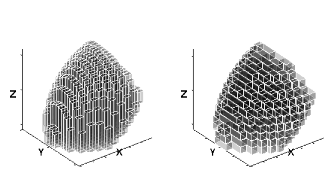
Figure 2: Two sample partitions of the convex hull of the SDSS data into cuboids with transverse size .01 redshift units. The long-axes of the cuboids are parallel to the z-axis and y-axis. These crude partitions are for illustration only; those used in the analysis are much finer.

For the grid size equal to .0001 redshift units (0.416 Mpc) the sum of the volumes of the cuboids matches the exact volume of the convex hull to one part in $10^{8}$, not surprising since this computation is equivalent to the elementary integral calculus procedure for computing the volume of the convex hull. Putting all this together, the result will be used to correct the galaxy Fourier transform for the effects of the data window – cf. Section 3.5. Appendix A describes a way to check how well the transform approximates the actual selection function, and Appendix B describes MatLab code implementing the Fourier transforms, including the deconvolution of the window transform, with a link to the code and data files in electronic form.

3.4 Fast Fourier Transform of the Binned Galaxy Distribution

Another way to estimate the Fourier transform is to construct a 3D histogram of the galaxy positions in a spatial grid of 3D bins, or voxels. To use the fast Fourier transform each voxel must be a cube with the same small size $\Delta x=\Delta y=\Delta z$. This procedure discards some information, due to rounding of galaxy coordinates and placing some close pairs in the same voxel. Table 1 summarizes statistics for three grid sizes. Columns 5-8, giving the maximum number of galaxies in any one voxel and the fractions with 0, 1, and 2 or more galaxies, are useful in assessing the information loss in this binning. Ideally the fraction with more than one galaxy would be zero, leaving coordinate truncation as the only error. Computation with 512 bins in each coordinate – case (c), with 135,005,697 voxels – seems to be the largest feasible with current personal computers. As the accuracy of the computation increases more and more voxels are empty, since the number not empty cannot exceed the number of galaxies. The last column gives the fraction of voxels empty because they are outside the survey volume; these values are large due to the shape of the survey and because we zero-padded it for good frequency resolution.

Table 1: Statistics for the Binned Fourier Transform

Case	$N_{\mbox{bins}}$	$N_{\mbox{vox}}$	$\Delta$	Max n	Fraction n=0	Fraction n=1	Fraction n $>$ 1	Fraction Outside
(a)	128	2.1 M	6.8	32	0.9693	.016519	.014221	0.8923
(b)	256	16.8 M	3.4	11	0.9938	.004882	.001300	0.9347
(c)	512	134.2 M	1.7	5	0.9991	.000869	.000062	0.9347

The Fourier transform of the window is simply that of this bin array with unity inside the sample volume and zero outside, cf. equation (3.3). Actually instead of the convex hull of the filled bins, for each dimension we assigned a unit value to each bin between the minimum and the maximum indices of bins containing galaxies in all of the corresponding x-columns, y-columns and z-columns. In practice this is essentially the same as the convex hull. The inverse transform of the Fourier transform computed this way is guaranteed to exactly reproduce the input counts-in-voxels, so there is no point in numerically demonstrating the accuracy of this representation as in Appendix A for the direct transform.

3.5 Deconvolution of the Data Window

We approach correcting for the selection function (or window) in a straightforward way. Functions of a 3D coordinate vector $\bf{x}$ related multiplicatively in the manner

$$q_{obs}({\bf x})=q_{true}({\bf x})q_{window}({\bf x})\ ,$$ (15)

have spatial Fourier transforms related by

$$Q_{obs}({\bf k})=Q_{true}({\bf k})*Q_{window}({\bf k})\ ,$$ (16)

where $Q_{obs}(\bf{k})$ is the Fourier transform of $q_{obs}(\bf{x})$, etc., and $*$ means 3D convolution on the vector $\bf{k}$. There are many deconvolution techniques for finding $q_{true}(\bf{k})$, thus correcting for the window function, but here the simple expedient of Fourier transforming Eq. (16) yields

$$q_{true}(\bf{k})=F^{-1}{F[Q_{obs}(\bf{k})]\over F[Q_{window}(\bf{k})]}$$ (17)

where $F$ and $F^{-1}$ are the forward and inverse Fourier transforms. In all numerical results presented here the MatLab (©MathWorks) multidimensional functions fftn and ifftn were used for both the direct and binned cases. This deconvolution method is sometimes avoided because of worries about noise amplification and/or issues when the denominator in eq. (17) is zero (or small in absolute value), but here these issues do not cause any serious problems.

4 Characterizing the Spatial Distribution of Galaxies

We are now ready to use the above Fourier transform methods for global characterization of the galaxy distribution. It is useful to compare results from the binned and unbinned Fourier transforms. Neither one is better in all aspects than the other. Of course they both have limited spatial frequency resolution, but their different data representations implement distinct approximations. The binned approach suffers from the information loss associated with quantization of the galaxy coordinates.

4.1 Fourier Power Spectrum

Figure 3 shows the deconvolved power spectra for both methods: direct as in Sections 3.2 and 3.3 and binned in Section 3.4. The powers projected in three orthogonal directions, $|F(k_{x},0,0)|^{2}$, $|F(0,k_{y},0)|^{2}$, and $|F(0,0,k_{z})|^{2}$, are distinguished by lines of different widths. These three power spectra share the same zero-frequency value, namely $|F(0,0,0)|^{2}=N^{2}$, and we have normalized the plotted curves to unity at zero spatial frequency – which of course is off-scale on these log-log plots. Comparison of the power spectra in different directions provides a simple measure of isotropy. The spectra at lower spatial frequencies approximate the power-law dependence characteristic of red noise (Aschwanden, 2011). The straight (dashed) lines in this figure are least-squares fits to the mean of the three power spectrum curves in the interval below the cutoff at log $k=-1.2$ mentioned in the caption; the log-log slopes indicated there are not far from the common red noise value of $\approx-2$. The scatter reflecting high variability at small scales motivates the vertical shifts in the higher frequency part of these plots, at the same cutoff used for the power-law fits.

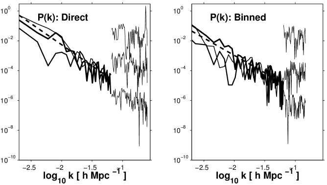
Figure 3: Power Spectra from deconvolved direct (left) and binned (right) Fourier Transforms: x, y and z powers in solid lines of increasing width. As in Fig. 1 the dimensionless power is shown divided by its zero-frequency value $N^{2}$ to yield P(0) = 1. Above log $k$ of -1.2 (spatial frequencies $>0.063$) the powers are multiplied by 3000, 10, and 0.1, respectively, for clarity. The dashed straight lines are power law fits to the low frequency data (averaged over the 3 directions) with slopes -2.8 and -2.3 respectively.

Figure 4 plots our power spectra against those from some other authors. In interpreting the figure and assessing this comparison the reader should bear in mind both the simplicity of our method – using the unadorned Fourier basis and avoiding the variety of known weighting schemes, corrections, and assumptions – and the differences in the data used. This figure compares the average of our three x, y and z projected spectra in Figure 3 with results from detailed analysis of very similar data by Tegmark et al. (2004b) and of a much larger sample by Percival, Nichol, Eisenstein et al. (2007).

Using a flux limited sample, instead of our more easily interpreted volume limited sample, the first authors address the selection function, redshift space distortions, bias effects and other systematic errors, using a Pseudo-Karhunen-Loeve expansion (Tegmark et al., 2004b). Figure 4 includes the data from the first two columns of their Table 2 in the form of open circles, without showing their rather large horizontal and vertical error bars. They refer to this as the real-space galaxy-galaxy power spectrum $P_{gg}$ in units of $(h^{-1}Mpc)^{3}$, and “recommend using column 2 for basic analysis.” Like ours this estimate treats the galaxies as equal points and accordingly is not corrected for bias, justified because bias appears to be largely luminosity and scale independent (their Figures 28 and 29, renormalizing to the linear $\Lambda$CDM model). It is noteworthy that their power spectra with and without correction for the Fingers of God (FOG) – their columns 2 and 3, respectively – would be indistinguishable had we plotted both. Even though the effect of FOGs seems insignificant here, redshift space distortions should be addressed in any serious scientific applications. Analysis of a much larger redshift survey, extending to much larger redshifts than our study, by Alam, Ata, Bailey et al. (2016), includes significant redshift-space distortion corrections. The results of a similarly detailed analysis by Percival, Nichol, Eisenstein et al. (2007) of a sample including both SDSS main galaxies and luminous red galaxies (LRGs) out to much larger redshifts ($z\sim 0.5$) than our sample, are plotted as plus-signs.

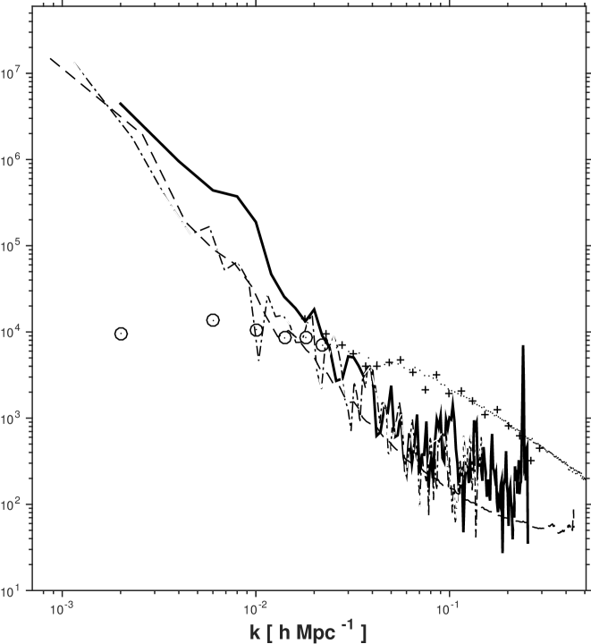
Figure 4: Power Spectrum Comparison. Solid line: power from average direct Fourier transform (eq. 5). Dots-dashes: average binned FFT. Dashes: average of the direct powers at all of the frequencies falling in a given 1D spherical volume in ${\bf k}$ space. Our power spectra are renormalized to units of $(h^{-1}Mpc)^{3}$ for comparison with the other authors, and corrected for the selection window (cf. Section 3.5). The spatial frequencies and powers from columns 1 and 2 of Table 2 in Tegmark et al. (2004b) are plotted as plus signs (+), and those of Percival, Nichol, Eisenstein et al. (2007) as small dots (but with the lowest 6 frequencies emphasized by circumscribed circles).

First compare the curves for the direct and binned transforms (solid and dot-dash lines). While the values at some frequencies, especially the lower ones, differ by nearly an order of magnitude, the rough similarity of the slopes and values at higher frequencies demonstrates that these two methods are crudely consistent with each other. As well, the similarity of some of the finer detail in the two representations support the notion that the effective spatial resolution is relatively good (probably better than that corresponding to Tegmark et al.’s horizontal error bars, not shown here). The differences between our spectra and the others, especially in the form of a vertical offset above about $k\approx.05$, are not surprising in view of the differences in the data and methods used.

Nominally the plotted points in our power spectra are independent of each other. Essentially no significant measurement errors propagate into this plot at any spatial frequency. The only large discrepancy in the plot is between Percival et al.’s and our powers at the longest scales, understandable in terms of the difference of the data samples and systematic effects at large scales. In the power spectra in Tegmark et al. (2004b) and ours, not surprisingly there is no evidence for baryon acoustic oscillation features. These important features do begin to appear at around $k=0.7Mpc^{-1}$ with the larger sample and the inclusion of the SDSS luminous red galaxies in (Percival, Nichol, Eisenstein et al., 2007).

A further avenue of investigation would invoke surrogate redshift surveys, such as galaxy catalogs derived from $N$-body simulations. The idea would be to compare simulated against actual distributions of variously grouped power or phase spectrum quantities. Using ensembles of synthetic catalogs to enable variance analysis is probably a fruitful path to reliable scientific conclusions. While such a study is beyond the scope of this paper, we have carried out a simple comparison against a single catalog, the Millennium Simulation (MS) of Springel et al. (2005). This $N$-body simulation (with $N=2160^{3}=1.0078\times 10^{10}$) contains data used to study multi-scale structure in Papers I and II. The $xyz$ positions of simulated galaxies were treated in the same way as the SDSS data – yielding a volume limited sample, and without discarding galaxies lying close to the edges of the data space. This MS analysis is described in Section 5.

4.2 Gaussianity

In modern cosmology it is often posited that the initial conditions of the Universe consisted of a random density distribution described as a Gaussian random field. It is not completely clear how the character of such an initial distribution may have evolved gravitationally, or how matter-to-galaxy biasing, integrated Sachs-Wolfe (ISW) effects, and gravitational lensing may complicate conclusions based directly on the galaxy distribution (Coles, 2000). Hence the interpretation of detected non-Gaussianity (NG) in the distribution of low redshift galaxies would not be straightforward. We find no NG signatures here, but if significant detections were to be made, e.g. in future large redshift surveys, the resulting parameters would be useful as additional constraints on precise cosmological evolution models. Hence we now describe some aspects of direct analysis of the Fourier phase spectrum.

Although Gaussian processes are well understood mathematically, the elusive nature of non-Gaussian (NG) processes has complicated and discouraged exploration of searches for their signatures. The infinite number of ways a process can depart from Gaussianity leads to a plethora of potential NG metrics, only a handful of which have been pursued. Here we describe a relatively straightforward class of NG tests based on metrics of Gaussianity applied to the complex Fourier data cube. The idea centers around metrics of how identically and independently (IID) the Fourier phases at different spatial frequencies are distributed.

Much previous work centers on parametric tests, valid only in the context of hypothetical physical or mathematical models and thus far short of general characterization of NG. Analyses using higher-order spectra and correlation functions, or function bases such as Karhunen-Loeve expansions (Vogeley and Szalay, 1996; Tegmark et al., 2004b) or harmonic oscillator eigenfunction expansions (Rocha et al, 2001) are closer to the spirit of non-parametric analysis with its greater generality and flexibility. On the other hand these methods are simply ad hoc ways to project an infinite dimensional function space into lower dimensions for modeling convenience. By contrast the approaches of Rocha et al (2001) and Contaldi et al. (2000) employ Bayesian frameworks that alleviate some of this ad hoc character. But the conclusions are still dependent on the correctness of a hypothetical model (e.g. the quantum mechanical harmonic oscillator in Rocha et al (2001)). More recently Kovács, Carron and Szapudi (2013) define generalized phases and apply this concept to characterize the coherence between WMAP and Planck CMB maps.

In the CMB context various authors have made suggestions for the two aspects of this problem, namely identification of: (a) phase subsets that are computationally practical but do not discard too much information, and (b) non-Gaussianity metrics for these sets (Chiang et al., 2003; Chiang, Naselsky and Coles, 2004; Naselsky, Chiang, Olesen and Novikov, 2005; Chiang and Naselsky, 2007). For one example Chiang, Naselsky and Coles (2004) discuss a number of general problems and propose an innovative procedure using return maps. This can be thought of as a way to quantitatively characterize joint distributions (cf. Scargle, 1990, e.g.). In another example Chiang and Naselsky (2007) propose ring-like sets in spatial frequency space. And more recently several authors have proposed phase analysis based on 3-point correlation functions of the Fourier transform of a whitened version of the density field (Wolstenhulme, Bonvin and Obreschkow, 2015; Eggemeier et al., 2015).

4.2.1 The Fourier Phase Spectrum

We utilize the Fourier transform as a convenient setting for quantitative characterization of the Gaussianity of the spatial distribution of galaxies. Keep in mind that the histograms constructed in pursuing this goal are simply distributions from the one data sample on hand – not probability distributions with respect to some stochastic ensemble. Several considerations motivate our focus on phases:

1. The phase spectrum captures much of the information on non-Gaussianity present in the data.

2. Phases of Gaussian data are identically and independently distributed (IID; see e.g. Naselsky, Chiang, Olesen and Novikov, 2005). Measures of dependency in the phase distribution are consequently measures of non-Gaussianity.

3. The oft used bi-spectrum and higher order spectra and correlation functions have many problems.

4. In most practical, largely non-astronomical, situations the Fourier phase information in 2D images is much more important than the amplitude information (Oppenheim and Lim, 1981; Coles, 2000; Chiang and Coles, 2000a). See also (Mannell, 1990) for a related discussion of phase in speech intelligibility.

In addition see comments in Section 6 regarding related statistical methods to be pursued in future work.

Point number 3 deserves more explanation. Several authors (e.g. Ferreira and Magueijo, 1997; Carron, 2011; Carron and Neyrinck, 2012; Carron and Szapudi, 2015) have disclosed a variety of fundamental problems with the multi-point correlation function hierarchy, including large computational complexity that grows rapidly with order, information mixing among the orders, and the fact that even including all orders only incomplete information is captured for a log-normal density field (Carron and Neyrinck, 2012) and only a tiny dramatically decaying fraction of the total information content of large fluctuations (Carron, 2011). A direct Fourier transform avoids to a large degree all of these problems: computational complexity is relatively small ($N\times$ the number of spatial frequencies), the amplitudes at different spatial frequencies are independent of each other, convergence is well understood, and the invertibility of the Fourier transform (Appendix A) assures that the combination of the power and phase spectra capture all of the information in the data. Most important, simple data cubes cleanly display phase as an explicit function of $\bf{k}$. Furthermore there are no special problems like those with generating representative sets of triangles and avoiding oddly shaped ones, as for 3-point estimators.

Coles (2000) gives a clear discussion of the background for these points, to which we add only a few remarks. Of course the basic notion is that the Fourier Transform appraises structure as a function of scale. The discrete estimate is a finite sampling of a potentially infinite number of degrees of freedom. But the Nyquist-Shannon sampling theorem guarantees that it captures all the information contained in the data, limited only by the data resolution. Since the inverse Fourier transform exactly recovers the raw data, it is clear that the (frequency dependent) amplitudes and phases contain complementary information, together yielding a complete description of the data. The Fourier power spectrum completely characterizes the Gaussian properties of the data; while non-Gaussianity information can appear in both amplitude and phase spectra, in many situations the latter dominates.

Driven by these comments our basic approach is to study phase distributions for non-uniformity. Perhaps the simplest possible approach is to examine the overall distribution of phases without regard to spatial frequency. Any structure in this distribution would suggest the presence of underlying non-Gaussianity.

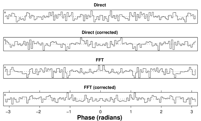
Figure 5: Distributions of phases for the four cases (Direct as in eq. (4), and simple FFT of binned data as in Section 3.4, both with and without correction for the window function, as labeled). Horizontal axis is phase in radians. The vertical axis is the 129-bin histogram population of phases from the $128\times 128\times 128$ 3D phase cube, with a horizontal dotted line at the expected rate of $128^{3}/2\pi=333,772.1$ counts per radian, the ranges of these plots are $12,000$ is the same units. Poisson count error bars for a typical bin are shown in the upper left corner of each plot.

Figure 5 shows simple histograms of all 16 million-plus phases for the four cases, with 256+1 spatial frequencies in all 3 dimensions. If these plots were scaled to include the zero of the ordinate the fluctuations would be invisible. There is here no evidence for any departure from uniformity, but these overall distributions are almost certainly insensitive to NG because they do not take account of frequency relationships, which are discussed in the next section.

It is perhaps notable that even the distributions for phases uncorrected for the data window (the first and third panels) do not reveal perceptible nonuniformity. This somewhat surprising result probably reflects that the data window truncates the Fourier components but does not change their phases.

4.2.2 Distributions of Phases Grouped by Spatial Frequency

A more refined approach is to aggregate phases into two or more sets and test whether the distributions in them are identical, as they should be in the Gaussian case. The model-independent and non-parametric way the phase spectrum neatly lays out the relevant information in a 3D data cube facilitates such segmented analysis. Accordingly we use the following procedure to study NG:

(a)

Compute the complex 3D Fourier transform $A(k)e^{i\phi(k)}$.

(b)

From (a) compute the 3D data cube $\phi(k_{x},k_{y},k_{z})$.

(c)

Specify a collection of subsets of (b) to be tested.

(d)

Evaluate differences of nearest-mode phases within each member of the collection (c).

(e)

Select an IID metric and compute it for each of the differenced arrays in (d).

(f)

Assess the statistical significance of the results of the collection of tests (e).

The first two steps are straightforward from the discussion in Section (3). Step (c) addresses the need to identify sets of frequencies related to each other in some germane way. For example phases at nearby frequencies would presumably show dependencies when those at well-separated frequencies might not. From among the many possible ways to take advantage of the organized way frequencies are arranged in a 3D phase-data cube, we adopt the following: Let $N_{k}$ be the size of the Fourier transform in each of its 3 dimensions. For each of the $N_{k}^{2}$ pairs $(k_{y},k_{z})$, for the array consisting of the corresponding $N_{k}$ phase values as a function of $k_{x}$ – we call this array an $x$-beam – compute a metric or test statistic $T_{x}$, and similarly for $y$-beams and $z$-beams.

Step (d) implements suggestions in (Chiang and Coles, 2000a; Coles and Chiang, 2000, 2001; Coles, 2000; Watts, Coles and Melott, 2003) emphasizing the potential effectiveness of studying the differences between phases at adjacent spatial frequency modes, as opposed to the phases themselves. Consider one dimensional first differences of the form

$$D_{k}=\phi_{k+1}-\phi_{k}\$$ (18)

where $k$ is a spatial frequency index, here taken in one of the three cardinal directions – x, y or z. The following analysis was done with un-differenced, first-differenced, and higher-order-differenced beams, the latter proving useful in unrelated sequential analysis problems (unpublished). But un-differenced or higher-order differences gave less clean results than first differences, so here we report only these results.

As noted by Watts, Coles and Melott (2003) if the phases are IID on the circle then so are their differences. This requires that the phase differences that lie outside $(-\pi,\pi)$ first be adjusted for “wrap around” as follows:

$$D_{k}^{m} \rightarrow+2\pi-D_{k}^{m}\ \ \mbox{for}\ \ D_{k}^{m}>+\pi$$ (19)

$$\rightarrow-2\pi-D_{k}^{m}\ \ \mbox{for}\ \ D_{k}^{m}<-\pi$$

This procedure is different from standard phase unwrapping based on changing absolute jumps greater than $\pi$ to their $2\pi$ complement (e.g. for the MatLab function unwrap; © the MathWorks Inc).

Step (e) amounts to the generation of a collection of estimates of a NG metric of a beam in the form

$$F_{x}(k_{y},k_{z})=T_{x}\phi(k_{x},k_{y},k_{z})\ \ k_{y}=1,2,\dots,N_{k};k_{z}=1,2,\dots N_{k}\ ,$$ (20)

where the subscript just indicates which variable $T$ operates on. At this point a huge range of possible definitions of $T$ opens up. There is no unique or universally best metric, and undoubtedly different metrics are suitable for different forms of NG. Item (2) in Section 4.2.1 motivates the use of a test statistic for the null hypothesis of IID phases. The formal definition of independence (joint distribution equals product of individual distributions) is difficult to turn in to a practical IID test (e.g. Scargle, 1981; Coles, 2000; Hyvärinen, Karhunen and Oja, 2001, and Section 6 below). Variance is a simple and easily interpretable statistic that might be sensitive to some types of NG. The Planck Collaboration studied both skewness and kurtosis (Ade et al., 2014) – measures of asymmetry of a distribution and of the relative importance of the center versus tails. Jin et al. (2005), based on detailed study of various methods of CMB non-Gaussianity detection, concluded that analysis of the kurtosis of wavelet coefficients is best. Based on an idea in Polygiannakis and Moussas (1995), Chiang and Coles (2000a) propose use of phase entropy for NG studies. Hyvärinen, Karhunen and Oja (2001) claim the optimality of entropy as an NG metric, but in practice use kurtosis as an approximation because of pitfalls in entropy estimation. Skewness did not seem to add any NG detective efficiency compared to kurtosis, so here we report studies of variance, kurtosis, and entropy. In every case these metrics were applied to first differences between phases at adjacent frequencies.

4.2.3 NG Metric Maps: Control Samples

Consider now the analysis of synthetic NG-free data for a sequence of three increasingly realistic sampling schemes, followed by analysis of the actual data. Maps of the beam metrics defined in Eq. (20) are presented as images with greyscales of the metric defined along one dimension, as a function of the two perpendicular dimensions in the phase data cube. Within each of the following figures the three panels present the analysis of the same data for beams in the x, y and z directions. When the data fall within the irregularly shaped volume we have used different spatial frequency arrays in the three directions. That is, the frequencies are integer multiples of a fundamental frequency defined by

$$k_{0}(n)={2\pi\over L_{(n)}}\ \$$ (21)

where $L_{(n)}$ is the range of the data in coordinate direction $n$. This choice gives slightly better deconvolutions. In contrast, for convenience the power spectra presented above in Section 3 refer to the same frequency array in all directions, namely corresponding to the largest of $L_{x},L_{y},$ and $L_{z}$.

Figure 6 contains maps generated from a single 3D random phase cube. Such images are used throughout this section to visually search for possible non-random patterns in the behavior of NG metrics computed along beams parallel to the coordinate axes. The rows of panels are for the three metrics – variance, kurtosis and phase entropy – applied to the first differences of the phases adjusted as in Eq. (4.2.2). The columns are for the statistics computed along the x, y and z directions. These unsmoothed

plots retain the discrete nature of the data to allow better appreciation of the randomness of the distributions. The data cube generating this figure consists of phases generated directly from an IID random number generator, not from a Fourier transform, and thus represents the simplest and most extreme form of the null hypothesis of IID phases. As expected there is no apparent structure in any of these panels.

Figure 6: Maps of NG metrics for random phases. All images are from the same 3D $128\times 128\times 128$ cube of data consisting of IID random numbers uniformly distributed on $(0,2\pi)$. Columns from left to right: beams in the x, y and z directions. Rows (top to bottom): variance, kurtosis and phase entropy. Coordinates are indices in the synthetic random arrays, not functions of spatial frequency as such, so axis labels are suppressed. Here and in subsequent figures the grayscale bars to the right of each panel depict the range of the metric.

Figure 7 shows the same type of map as in Figure 6 but here the phases are derived from the direct Fourier transform in Eq. (5) of random points distributed uniformly within a $xyz$ cube. This configuration is chosen to diagnose possible modification of the phase distribution inherent in the transform procedure, but with a window that is benign due to the simplicity of its boundaries. Deconvolution of the data window is not relevant, due to the simplicity of the boundaries of the data space. As expected there is no apparent structure in any of metrics presented in these panels.

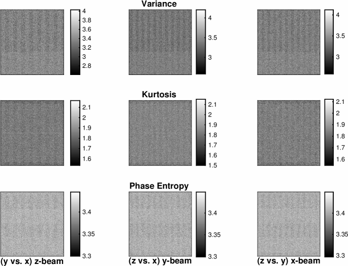
Figure 7: NG statistics maps for phases of the direct Fourier transform of a set of $100,000$ xyz points randomly and uniformly distributed within a cubic 3D volume, using equation (5). The identities of the panels are as in Figure 6. While the coordinates are now spatial frequencies, the units are fixed by the arbitrary size of the cube, and therefore are also arbitrary. The $128$ frequencies shown here cover the range $-f_{\mbox{0}}$ to $f_{\mbox{0}}$, where $f_{\mbox{0}}$ = $2\pi/L$ is the fundamental frequency and $L$ is the cube size; zero frequency is the point at the very center of the plot, as in all the subsequent figures.

Figure (8) presents phase analysis for xyz-data that are still synthetic random points but now distributed uniformly within the convex hull of the actual data. The idea is to diagnose possible structure in these maps induced by the irregular boundaries of the data space. The lack of structure here indicates that such distortion is minimal.

Figure 8: Variance (first two rows), kurtosis (middle pair of rows) and phase entropy (last two rows) maps for phases from the Fourier transform of 139,798 xyz points (the same as the number of galaxies in our SDSS data set) randomly distributed within the convex hull of the actual data. The members of each of these pairs are without and with data window deconvolution, respectively. Columns are the 3 projections as in previous figures.

4.2.4 NG Metric Maps: The Galaxy Data

Now turn to the actual galaxy data. Figure 9 presents the same analysis as carried out for the last of the control cases in the previous section. The maps in the first, third and fifth rows, depicting the statistics for the phase cube not corrected for the data window, show clear evidence of structure – most evident for the y-beam in the middle row.

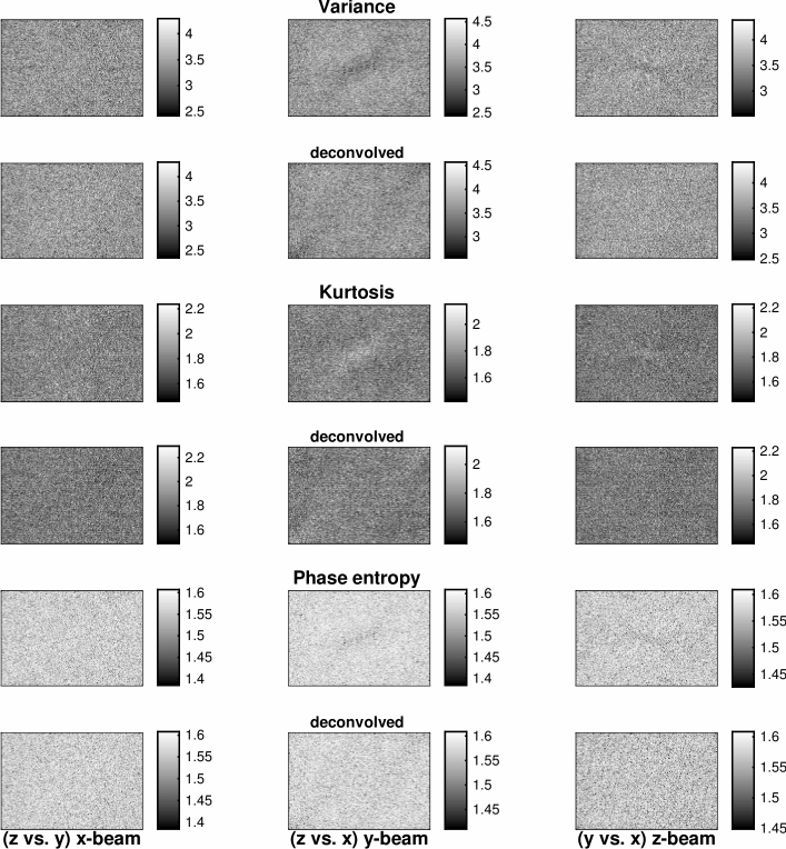
Figure 9: NG maps from the Fourier transform of the actual 139,798 galaxy positions, displayed as in Fig. 8. Note that the kurtosis structure is lighter than average, as opposed to the darker than average features in the other two cases. The centers of the linear scales of 128 frequencies are 0; the adjacent points are $\pm 0.002\mbox{Mpc}^{-1}$; the ends of the scale are $\pm 0.128\mbox{Mpc}^{-1}$.

The null results with the control samples in the previous section suggest that this structure is not due to the irregularity of the data window alone – no non-random structure is evident in Figure 8 – but rather to the combination of both the multi-scaled clustering in the point distribution and the irregular shape of the data window. In any case, the structure in all three beams (rows 2, 4, and 6) largely disappears when the data window has been deconvolved in the spatial frequency domain.

The subtle residual structure is possibly real, but more likely reflects imperfect deconvolution and is therefore not of astrophysical interest. This conclusion is reinforced by the similarity of the morphologies of the uncorrected and residual structure. Figure 9 is simply illustrative of an approach to a difficult scientific problem – perhaps useful in future studies with larger data sets – and is of course not a definitive comparison of the three statistics nor meant to imply that kurtosis or variance are superior metrics. Indeed Hyvärinen, Karhunen and Oja (2001) present evidence that entropy may be an optimal Gaussianity detector (cf. Section 6).

4.2.5 Phase non-Gaussianity due to Density Perturbations

Under gravitational evolution from even a perfectly Gaussian initial state the low-redshift galaxy distribution is likely to have developed some degree of departure from Gaussianity. Hence more realistic tests of NG detection methodologies would involve simulated density perturbations. This section explores the connection between the distribution of phase differences and nonlinear clustering (cf. Watts, Coles and Melott, 2003).

We generated synthetic data consisting of points randomly distributed in cylinders superimposed on a uniform background within a unit cube. These structures are not meant to be realistic models, for example of cosmic strings or other topological defects; they are constructed as pseudo-acoustic, transversely confined waves to introduce some degree of disturbance to the Fourier phases. Each cylinder contains points drawn randomly from normal distributions with variance $0.005$ in the transverse directions (x and y), and proportional to $1.1+\mbox{sin}(kz)$ longitudinally. Fig. 10 depicts these cylinders: one is parallel to the z-axis; a second is slightly tipped ($\approx 1^{\circ}$) and the third even more so ($\approx 6^{\circ}$)).

Figure 10: Density perturbations inserted into a unit 3D data cube. Coordinates of the end points of the three cylinders: #1: (0.5,0.5,0.0) - (0.5,0.50,1.0); #2: (0.5,0.7,0.0) - (0.5,0.72,1.0); #3: (0.8,0.7,0.0) - (0.9,0.72,1.0). Transversely within each cylinder the points have a normal distribution of standard deviation $0.005$. The longitudinal density modulations correspond to sinusoids $1.1+sin(kz)$ with $k=50,64$ and $45$ – i.e. approximate periods of 0.12, 0.10 and 0.14 units. For visual clarity only $1,000$ points per beam are shown; many more were used in the simulations as indicated in the figure captions below.

Realizations of this configuration were superimposed on a dense random background of uniformly distributed points, the former representing a perturbation of the latter. The columns of Fig. (11) display distributions of phase differences

$$D(k_{x}|k_{y},k_{z})=\phi_{k+1,k_{y},k_{z}}-\phi_{k,k_{y},k_{z}}$$

$$D(k_{y}|k_{x},k_{z})=\phi_{k_{x},k+1,k_{z}}-\phi_{k_{x},k,k_{z}}$$ (22)

$$D(k_{z}|k_{x},k_{y})=\phi_{k_{x},k_{y},k+1}-\phi_{k_{x},k_{y},k}$$

Figure 11: Normalized distributions of nearest mode phase differences for random points in a 3D data cube with various numbers of points drawn from the cylindrical configuration of Figure 10. The twelve thin lines represent the distribution for the following numbers of points in each cylinder: $10,32,100,317,1000,3163,10000,31623,100000,316228,1000000,3162278$, against a uniform background of $10,000,000$ uniformly distributed points. The thicker curves are for background only (top) and no background (bottom, $3162278$ points per cylinder). The curves are shifted vertically for clarity; mean and zero levels are indicated by horizontal dotted lines and circles at the curve endpoints, respectively. Compare with Fig. 1 of Watts, Coles and Melott (2003).

in the three indicated directions. From top to bottom the vertical sequences exhibit the evolution of the distribution with increasing NG signal strength. As expected, for weak signals the distributions are flat, but as as the NG signal strength grows the distributions are more and more distorted. At the seventh case (out of 12), with $10,000$ points in each of 3 cylinders, the distortion starts to become clearly significant.

Plotted in the same way as Figures 6-9, the maps in Figure (12) for the pure density signal (only points in the cylinders, no background), indicate that all three of these statistics reveal distinct spatial frequency structure. The maximum frequency in the Fourier transform gives a minimum scale somewhat larger than the approximate width of the cylinders; therefore the plots do not resolve these structures but reflect the larger scales associated with distances between the cylinders, etc.

Figure 12: Phase statistics maps for the toy three-cylinder density data described in Figure 10, displayed as in Figures 6-9. The axis scales comprise 65 frequencies, with 0 at the center; the spatial periods corresponding to the maximum $|k|$ are 0.0312 in units where the cube edges are of length $1$.

Figure (13) is for the case from the sequence in Fig. (11) where the weakest NG signal is just barely detectable in the difference distribution: $10,000$ points in each of the three cylinders, with a background of $10,000,000$ uniformly distributed points. The three cylinders together thus contain the fraction $0.003$ of the background. The volumes of the cylinders are approximately $\pi(2\times.005)^{2}$ – smaller than the cube’s volume by a factor of $3\times 10^{3}$ – so the point density in the cylinders is about $3$ times the mean density of the background.

Figure 13: Phase statistics maps for the toy three-cylinder density data described in Figure 10, displayed as in Figures 12. This figure illustrates what a barely detectable NG signature of the toy signal in Fig. 10 might look like, but of course is not a guide to realistic expectations.

This section developed a visual approach to assessing distributions of statistical parameters in a 3D data cube, and applied it to try to detect departures from the hypothesis of IID Fourier phases. In such displays the eye is famously good at perceiving patterns, but also easily fooled by noise fluctuations. Given the display issues of pixelization, contrast, range, color, non-linear scaling, etc., and the difficulty of rigorous analysis of statistical significance of perceived patterns in this kind of image, a more objective approach is called for, as addressed in the Epilog, Section 6.

5 Uncertainty

An estimate of the uncertainty of a scientific result is an important part of its value. At issue is how widely the result might vary on account of the inevitable accidental aspects of the measurement process. This can be addressed by appraising data values that could have been obtained but, by happenstance, were not. Cosmology often sidesteps its one-universe handicap by measuring uncertainty as the variance over a postulated distribution function of such hypothetical data. In this section we discuss uncertainty in our results using several ideas of what constitutes such “other data,” in turn considering observational, internal and external errors.

5.1 Observational Errors

One often has relatively good information about observational errors. E.g. normal distributions with well-determined parameters can often be theoretically justified and empirically tested and calibrated. Assessment of the corresponding uncertainty is then relatively straightforward. The only sources of observational error relevant to our analysis are fiber collision effects and random measurement errors in coordinates and redshifts. Paper II discussed our procedure for mitigating the former, and we now demonstrate that the latter are negligible.

We simulated 100 realizations of normally distributed heteroscedastic errors (zero mean and standard deviation as given for each galaxy in the data catalog) added to the actual right ascension, declination and redshift values. Power spectra for these data sets were carried out exactly as for the actual data. The relative errors were computed as the standard deviations of the resulting powers divided by the corresponding means. Figure 14 plots these results as functions of spatial frequency. These relative errors are maximum at the highest spatial frequencies, reaching at most $1\%$. Overall the effect of these errors is at least several orders of magnitude too small to have any relevance. At the same time this analysis has ignored systematic errors and the likely possibility of correlated errors induced by systematics. In principle a similar display of phase uncertainty is possible, but difficult to display and relatively uninformative, so we do not present it.

Figure 14: Relative uncertainty from propagation of the observational coordinate errors. The ratio of the standard error to the mean of the power spectrum is plotted against spatial frequency. Solid line with dots, dashed line with squares, and dot-dashed line with circles: power in the x, y, and z directions, respectively.

5.2 Internal Variance

An additional element of uncertainty arises because, not only could the measured galaxy coordinates be different (as discussed in the previous subsection) but the sample could have actually contained different galaxies. The view is that the galaxy samples are randomly drawn from a hypothetical spatial distribution. The relevant uncertainty is termed internal variance – that is, internal to the data space at hand. One can think of this process as 3D spatial shot noise. This term typically refers to random fluctuations in a measured light curve of a varying astronomical source, but here the discreteness refers to galaxies instead of photons.

One could compute variances in ensembles of random draws from a model of this distribution. Shortcomings of any such model-based approach include loss of information by imperfect representation of the data, imposition of incorrect information (e.g. by effective smoothing), and dependence on the correctness of the model form and its parameter values. Furthermore this procedure provides no evidence on what the distribution actually is. Hence we do not choose to follow this approach.

Happily, random resampling techniques such as bootstrap and jackknife methods (Efron and Tibshirani, 1993) enable straightforward model-independent estimation of internal variance. Like most purportedly powerful and easily implemented algorithms, these methods are sometimes misunderstood and used carelessly. Two common reactions are that they are “useless; they seem to get something for nothing” or “great; they capture all relevant statistical information from all kinds of data.” The truth is in between but closer to the latter. The following discussion shows what resampling can do here and what it can’t.

The referenced resampling methods use the empirical distribution function (EDF) to approximate the true distribution described above. This function, derived directly from the data, captures all information contained therein about the true distribution. Galaxy-by-galaxy resampling with replacement or leave-one-out cleanly implement the bootstrap or jackknife principle, respectively. Resampling has the advantages that it relies on only the data measured, needs no additional data, and makes no assumptions other than that the empirical distribution is a good approximation of the actual one.

The jackknife method uses a set of samples, each consisting of the full data set with with one point at random removed. The bootstrap method seeks the approximation mentioned above with random draws from the EDF, defined to be the set of 3D coordinates $\{\mbox{\bf x}_{1},\mbox{\bf x}_{2},\dots,\mbox{\bf x}_{N}\}$ each assigned the probability ${1\over N}$, much as in Equation 3. The result is simply a sample, typically $N$ in size, randomly drawn with replacement from the original data points. That is, the randomly drawn galaxies are not discarded and may occur two or more times in the bootstrap sample. In both cases one simply analyzes many realizations of these surrogate data samples in the same way as the actual data. The correctness of the results relies on the single assumption that the empirical distribution function fairly represents the underlying physical process. The bootstrap bias or jackknife bias are estimates of any bias inherent to the algorithm. They compare the resampled mean against the original mean. However they can say nothing about possible bias in the original data themselves.

For the current power spectrum analysis the leave-one-out procedure of the jackknife is almost trivial to implement; the $m$-th jackknife sample, i.e. with the $m$-th point left out, is from Eq. (4):

$$F_{\mbox{jackknife}}(\bf{k},m)=\sum_{n\neq m}^{N}\ e^{-i\bf{k}\cdot\bf{x_{n}}}=F(\bf{k})-e^{-i\bf{k}\cdot\bf{x_{m}}}$$ (23)

Thus Fourier transforms of the jackknife samples can be computed without the need to evaluate the full $n$-sum each time. Bootstrap samples are only slightly more complicated. These computational efficiencies allow the luxury of using $N$ resamples – the maximum possible for jackknife and certainly overkill for bootstrap.

One more computational detail deserves mention: The replacement aspect of bootstrap resampling yields the potential of algorithm problems with exact data point duplicates. E.g. the local event rate measure $1/(t_{n+1}-t_{n})$ in time series applications (cf. Scargle et al., 2013) is infinite for duplicate event times. Here there are no such singularities, as the corresponding terms in the Fourier sum simply add without difficulty. Any concern is further alleviated since our bootstrap results are essentially identical to those using the jackknife, which does not generate duplicates.

Reporting variance for a 3D spatial distribution is notoriously difficult; instead we choose to report it for power spectra. Figure (15) displays bootstrap means, variances and biases for our standard SDSS galaxy sample. It is clear that the bootstrap components of internal variance and bias are quite small, especially at low spatial frequencies. The bottom panels are similar plots for bootstrap analysis of the comparable Millennium Simulation sample detailed in Papers I and II. Crudely speaking the results are similar, although the synthetic data yield somewhat less noisy power – with smaller variance and bias.

Figure 15: Bootstrap mean, variance and bias of power spectra. Left: x, y and z projections of bootstrap mean power (in order of decreasing darkness and as labeled) are plotted as narrow lines embedded in greyscale bands depicting the $\pm 1\sigma$ bootstrap standard deviation. Right: fractional bootstrap bias. Top panels: 139,798 bootstrap samples of the galaxy data. Bottom panels: similarly for the Millennium Simulation data. Jackknife results are indistinguishable from these.

5.3 External Scatter: Cosmic Variance

Survey data from different regions of the Universe give different parameter estimates. Such cosmic variance refers to errors in cosmological parameter estimates for scales larger than covered by a given survey. This uncertainty is in addition to those discussed in the above sub-sections. To estimate the effect of cosmic variance on our results we Fourier analyzed ensembles of sub-sets of two data sets.

The first, drawn from the SDSS DR13 (SDSS Collaboration et al., 2016), is significantly larger than the original DR7 selection of Paper I. It was obtained with a very similar query from the SDSS skyserver casjobs web interface, except that the absolute magnitudes were obtained directly in the casjobs query, whereas in Paper I we had to obtain this information via a cross match to the SDSS NYU VAGC catalog (Blanton et al., 2005). To further increase the size of the sample, while mostly remaining within the precepts of the data selection of Paper I, we adopted a somewhat larger redshift range ($0.005\leq z\leq 0.15$), and defined the volume limited sample with a slightly fainter cut in absolute R magnitudes, at -19.8495 instead of -20.1 as in Paper I. In addition we discarded galaxies with anomalously large R magnitude errors, adopting a threshold of 0.2786. As in Paper I we selected only the contiguous north galactic cap region and applied the same procedure to address the fiber collision bias. The resulting data set consists of $N=370,847$ galaxies in a (convex hull) volume of $100.7\times 10^{7}\mbox{mpc}^{3}$.

The second data set is the same one used in the current paper and defined in Paper I, roughly $2.6$ times fewer galaxies in a volume $10$ times smaller: $N=139,798$ and (convex hull) volume of $9.4676\times 10^{7}\mbox{mpc}^{3}$. In both cases these main data sets were subdivided into 8 independent subsets: octants, with divisions at the median values of the xyz coordinates. Summary statistics for these subsets appear in Table 2.

The top panel of Figure 16 shows linear plots of the power spectra, averaged over the 8 octants (as well as the three coordinate projections). The error bars are the standard deviations, which serve as estimates of cosmic variance in the spatial power spectra. The DR13 sample has somewhat smaller scatter, as expected on account of its larger size. The relative size of these uncertainties (standard deviation divided by mean) is plotted as a function of spatial frequency in the bottom panel. The cosmic variance of the power values at a given frequency are rather large, but one expects the more cosmologically relevant normalizations and logarithmic slopes of the spectra to be less uncertain, because they essentially average over this scatter as a function of frequency.

Figure 16: Cosmic Variance. Top: Linear plots of mean power spectra (averaged over 24 values: 8 octants $\times$ projections in the three coordinate directions) and corresponding standard deviations. Bottom: the above standard deviations divided by the means, as a function of spatial frequency. In both panels thin and thick lines are for DR13 and DR7, respectively.

That this is the case can be seen in the information on these parameters in Table 2. The 8 numbered columns refer to the octants, i.e. the independent sub-samples of the survey data described above. For the two data samples three quantities are tabulated for each octant: the normalization and logarithmic slopes from least-squares fits (linear in log-log space) to the spatial power spectra, and the number of galaxies in the octant. The next two columns give the corresponding means and standard deviations – first averaging the $x-$, $y-$ and $z-$ projections and then over the 8 octants.

We are interested in the uncertainties for the results derived in this paper for the full DR7 sample. Accordingly, the standard deviation values for the octants in the penultimate column are adjusted downward by the factor $\sqrt{8-1}$ to account for the relative sizes of the full and sub- samples, and reported in the last column (under the heading “This Paper”). The difference between the values for DR13 and DR7 data indicates the approximate uncertainty of these determinations and their extrapolation. The fact that the percentage variance in normalization is smaller than in slope may be related to the comment in footnote 9.

It is useful to compare these results with the quantification of cosmic variance by Driver and Robotham (2010). These authors studied the variance of galaxy density across independent subsets of much the same SDSS as used here. They derived approximate formulas for the corresponding standard deviation as a function the volume and aspect ratio of the 3D survey region, and the number of independent sight lines. Their Equation (1) gives the values reported in the second part of the last column, for density cosmic variance for our full DR7 sample. The close agreement between our $6.5\%$ (power spectrum slope) and their $7.0\%$ (galaxy density) for the average of the DR13 and DR7 extrapolations is probably partly due to the similarity of the data used in the two works and partly fortuitous.

Table 2: Cosmic Variance: Power Spectra of Octants

Octant	1	2	3	4	5	6	7	8	Mean	$\sigma$	Full DR7 Estimate
SDSS DR13											This Paper    Driver
Normalization	1.170	0.912	1.071	0.988	1.012	1.020	0.911	0.988	1.009	0.084	3.0%
Slope	-2.282	-1.817	-2.126	-1.910	-2.030	-2.022	-1.823	-1.953	-1.995	0.157	5.6%              8.1%
N (370,847)	47181	40143	50153	47946	49092	49005	38995	48329	46356	4290
SDSS DR7
Normalization	1.019	1.057	0.965	1.004	0.946	1.030	0.956	1.051	1.004	0.0432	1.5%
Slope	-1.937	-2.208	-1.692	-1.942	-1.629	-2.027	-1.714	-2.100	-1.906	0.209	7.4%              6.0%
N (139,798)	20408	11973	21697	15821	15903	21615	11891	20490	17475	4129

6 Epilog: Summary and Suggested Future Analysis

The unadorned 3D Fourier transform of coordinates from a redshift survey can be used to characterize the spatial distribution of galaxies, as demonstrated here with the volume limited sample defined in Papers I and II. A simple Fourier sum over the galaxy positions compares well with the transform of the same points binned in small 3D voxels. The direct sum has no resolution limit other than that inherent to the data or due to computational limitations. We display 3D Fourier power spectra, as well as projections radially and in three orthogonal coordinate directions; projection in arbitrary directions could provide a straightforward way to study isotropy.

However the emphasis here is on Fourier phase information, of interest for example in the context of Gaussianity measures. The phase spectrum has much to recommend it over the more commonly used multi-point statistics and related methods. We display maps (projected to 2D) of variance, kurtosis and entropy of nearest-mode phase differences to quantify distributional nonuniformity. Such analysis of the SDSS data, taking into consideration simulated control samples and the MS simulation, has not provided any convincing evidence for non-uniformity in the distribution of phases. This result is somewhat surprising since structure on any scale must generate local Fourier non-uniformities and render the distribution of density values (in spatial voxels) non-normal (e.g. Schaap, 2007). Furthermore even perfectly Gaussian initial density perturbations should suffer evolutionary modifications leading to nonGaussianity in the current distribution. On the other hand, offsetting these effects are data-analytic issues such as the rather conservative measures (e.g. phase differencing) we have been driven to, the ill-defined nature of the target signal, and the plethora of possibly relevant analysis methods – only a tiny fraction of which has been explored here or in previous research by others. In addition the normalization principle underlying the central limit theorem is at work in samples of any size.

However we expect that improved data – more recent SDSS data releases, deeper selections of other existing surveys, new larger ones, compendia of several redshift surveys covering similar redshift ranges, etc. – and guidance from theory and simulations will elucidate these issues, perhaps using phase analysis techniques augmented with the following three promising new approaches:

6.1 Optimal Phase Bins via Bayesian Blocks

The first problem is finding a principle for defining sets of phases to analyze. In an exploratory data analysis setting – i.e. absent guidance from theoretical predictions – one should, in principle at least, consider the set of all possible subsets. A way to address the exponentially large size of such a collection is to use the Bayesian Block algorithm (Jackson et al., 2005; Scargle et al., 2013) in its higher dimensional mode (Jackson et al., 2010) to optimally partition the phases. This $O(N^{2})$ algorithm yields the optimal among the $2^{N}$ possible binnings, where here the block cost function to be optimized would be some NG metric for the data within each block, for example kurtosis. This leads to …

6.2 Independent Component Analysis

… the second problem: the choice of NG metric. The close connection between independence and nonGaussianity (cf. Section 4.2.1) suggests that independent component analysis (ICA) will be useful. The wide-ranging but comprehensive monograph by Hyvärinen, Karhunen and Oja (2001) elucidates all of the NG issues discussed here and then some. By elaborating its slogan “nonGaussian is Independent” this monograph provides a unified picture of many inter-related properties of statistical processes – including dependence, correlation, Gaussianity, non-linear correlation, kurtosis, cumulants, and sparseness. This book and the update (Hyvärinen, 2016) detail related algorithmic approaches such as sparse coding, projection pursuit, principal component and independent component analysis. The existence of practical, fast ICA algorithms should facilitate application of these ideas to statistical cosmology. We are thus led to …

6.3 Large-Scale Inference: Higher Criticism and False Discovery Rate Control

… address the last step, inference. Recent advances in statistics have opened up a number of opportunities for future analysis of cosmological data. What Brad Efron calls “scientific mass production, in which new technologies … allow a single team of scientists to produce [very large ] data sets … ” has given birth to the field Large-Scale Inference (LSI). Two monographs (Efron, 2011; Efron and Hastie, 2016) review the statistical science underlying this discipline, its historical development, and its role in big data contexts. Two LSI techniques extremely popular in applied statistics, False Discovery Rate Control (FDRC) and Higher Criticism (HC), address problems potentially of great importance for large-scale astronomical data analysis. In the generic setting, termed large-scale hypothesis testing, one is faced with a large number of data elements, each providing evidence for or against a hypothesis (or possibly a different hypothesis for each datum). The analysis techniques, much like the trials factor, focus on integrative issues such as assessing the probability of making even one false rejection of a hypotheses in simultaneous analysis of $N$ hypothesis tests – especially in cases where the signal is expected to be weak (individual ones may not be detectable on their own) or rare (occurring in $\ll N$ of the cases).

Higher Criticism, perhaps more informatively termed second-level significance testing, was introduced by Donoho and Jin (2004), following John Tukey’s parable of the young psychologist, further developed in (e.g. Donoho and Jin, 2004, 2008, 2015; Walther, 2011) and applied in cosmology (e.g. Cayón, Jin and Treaster, 2005; Jin et al., 2005). The HC statistic may provide rigorous significance analysis of the multiple tests which are implicit in phase maps – effectively providing a statistical trials factor correction. HC applied to numerous beams within the phase-cube could lead to HC analysis of the HC statistic itself – third-level significance testing or even higher criticism. With somewhat different goals the FDR formalism, by controlling the relative proportion of false discoveries, can lead to more discoveries – useful especially when follow-up of putative discoveries is practical.

Appendix A Checking the Formalism using the Inverse Fourier Transform

It is useful to check how well our Fourier transform estimates capture the information in the galaxy coordinate data. The discrete Fourier transform of evenly spaced voxels is exactly invertible and therefore lossless, and so is the direct transform in Eqs. (4) and (5) in the limit of an infinite number of frequencies. Nevertheless it is of some interest to see how this limit is approached by comparing its inverse transform against the raw data. For this limited purpose a rough visual check suffices, since a precise goodness-of-fit metric, involving comparison of an effectively continuous representation with point data, is difficult.

In the direct transform there is no binning of galaxy positions, so if the Fourier transform were to be evaluated at an infinite number of spatial frequencies the inverse transform would exactly reproduce the data. That is the function

$$F_{x}(\bf{x})=\int F({\bf k})e^{-i\bf{k}\cdot\bf{x}}d\bf{k}$$ (A1)

would vanish except for unit delta functions at each of the galaxy positions. Normalization is not important here, so the factor ${1\over(2\pi)^{3/2}}$ sometimes written in front of the right-hand side of this equation is omitted. Inserting Eq. (4) into this expression we have

$$F_{x}(\bf{x})=\sum_{n=1}^{N}\ \int e^{-i\bf{k}\cdot(\bf{x}-\bf{x_{n}})}d\bf{k}$$ (A2)

It is well known that this integral is equivalent to a $\delta-$function at $x_{n}$, yielding the desired result.

It is useful to investigate how well these exact results apply to necessarily finite numerical computations. To do so we evaluate the expression

$$f(x,y,z)=\sum_{k_{x},k_{y},k_{z}}F(k_{x},k_{y},k_{z})e^{-i(k_{x}x+k_{y}y+k_{z}z)}$$ (A3)

appropriately normalized, against the raw data in Figure 17. The total number of spatial frequencies increases as the third power of the number of frequencies in each dimension, but it is nevertheless feasible to use a frequency grid that well resolves the relevant spatial structure in all three directions. The spatial frequencies were taken to be the usual integer multiples of the fundamental frequency of ${1\over 1082}Mpc^{-1}$. This denominator is approximately twice the maximum of the x, y and z ranges of the data, to eliminate wraparound.

Since the forward transform can be evaluated at any set of spatial frequencies, it is expedient to use an FFT algorithm to evaluate the expression above. We reconstructed 3D data points at every location in the $N_{k}\times N_{k}\times N_{k}$ array ($N_{k}^{3}$ voxels) where the value of $f(x,y,z)$ in equation (A3) exceeds a threshold. This threshold value was chosen to yield the same number of points (139,798) as in the raw data. The figure shows xy-projections of the points contained in a 12.5 Mpc thick slice in the z-coordinate, isolating roughly 5,000 points in all three panels. The limited frequency range dictates that the reproductions are smoothed representations of the galaxy data. The sequence in this figure demonstrates that increasing the number of spatial frequencies reproduces the discrete raw data with improved accuracy. Note that panel (c) with $N_{k}=256+1$ seems to have more points than (d) for $N_{k}=512+1$; in fact both have the same number, those in (d) more closely following the narrow filaments and other structures (with a consequent increase in overplotting of points) and therefore more faithfully reproducing the data. The key point is that information about the discrete structure at a broad range of scales, limited only by the resolution of the computation, is contained in the Fourier transform in eq. (5).

Figure 17: Comparison of x-y projections of thin (12.5 Mpc.) z-slices for (a) the galaxy data; and the corresponding reconstruction with the direct Fourier Transform in Eq. (A3) using (b) 128 frequencies; (c) 256 frequencies, and (d) 512 frequencies. Coordinates are in redshift units (rsu). The effective resolutions of the reconstructions are 16.9, 8.5 and 4.2 Mpc, respectively. Plots of other projections are very similar.

Figure 18: Reconstruction of the selection function. Top row: projections of the raw galaxy coordinates along the x- , y- , and z-axes respectively (empty white spaces indicate the extended ranges employed in the Fourier transforms) for comparison with the corresponding reconstructions via the inverse Fourier transform in the bottom row. These are 2D projections of thin slices oriented as indicated by the axis labels, with the gray-scale representing the reconstructed density. Here the grid size is .001 redshift units, for which the relative volume error in the cuboid representation is about one part in ten thousand.

In the same way the projected density plots in Figure 18 demonstrate that the inverse transform of the selection function Fourier transform is essentially a uniform solid corresponding to the observational data space. This procedure accounts for incorporating only galaxies inside the window, but of course does not in any way replace or estimate data outside of the window.

Appendix B 3D Fourier Transforms: MatLab Code

MatLab code (doi:10.5281/zenodo.432820) computes the Fourier transform of the galaxy coordinates, the corresponding window function and its deconvolution. The former is a direct evaluation of Equation 5; the latter is based on a refined partition of the actual data space – here taken to be the convex hull of the galaxy positions – into cuboids with $x$ and $y$ coordinates in an evenly spaced rectangular grid, as described in Section 3.3. More details are available in the ReadMe file and commented MatLab scripts at https://doi.org/10.5281/zenodo.432820

References

- Ade et al. (2014) Ade, P. et al. 2014, Astronomy and Astrophysics, 571, A23
- Alam, Ata, Bailey et al. (2016) Alam, S., Ata, M., Bailey, S. et al. 2016, The clustering of galaxies in the completed SDSS-III Baryon Oscillation Spectroscopic Survey: cosmological analysis of the DR12 galaxy sample, arXiv: 1607.03155
- Aschwanden (2011) Aschwanden, M. 2011, Self-Organized Criticality in Astrophysics: The Statistics of Nonlinear Processes in the Universe, Springer: Heidelberg.
- Bardeen et al. (1986) Bardeen, J., Bond, J., Kaiser, N., and Szalay, A. 1096, ApJ, 304, 15.
- Blanton et al. (2005) Blanton, M.R. et al. 2005, AJ, 129, 2562
- Bracewell (1999) Bracewell, R. 1999, The Fourier Transform and Its Applications, 2nd Revised Edition, McGraw-Hill, Inc., New York
- Cayón, Jin and Treaster (2005) Cayón, L., Jin, J. and Treaster, A 2005, MNRAS362, 826
- Carron (2011) Carron, J. 2011, ApJ738, 86
- Carron and Neyrinck (2012) Carron, J. and Neyrinck, M. 2012, ApJ750, 28
- Carron and Szapudi (2015) Carron, J. and Szapudi, I. 2015, What does the N-point function hierarchy of the cosmological matter density field really measure ?, arXiv:1508.04838
- Carron, Wolk and Szapudi (2015) Carron, J., Wolk, M. and Szapudi, I. 2015, MNRAS453, 450
- Chiang et al. (2003) Chiang, L., Naselsky, P., Verkhodanov, O. and Way, M. 2003 ApJ, 590, L65
- Chiang and Naselsky (2007) Chiang, L. and Naselsky, P. 2007, MNRAS, 380, L71
- Chiang and Coles (2000a) Chiang, L. and Coles, P. 2000, MNRAS, 311, 809
- Chiang, Naselsky and Coles (2004) Chiang, L., Naselsky, P., and Coles, P., 2004, ApJ, 602, L1
- Coles and Chiang (2000) Coles, P. and Chiang, L. 2000, Nature, 406, 376
- Coles (2000) Coles, P. 2000, Large-Scale Structure, Theory and Statistics, p. 593, in Phase transitions in the early universe: Theory and observations. Proceedings, NATO ASI, International School of Astrophysics ’Daniel Chalonge’, 8th Course, de Vega, H. J., Khalatnikov, I. M. and Sanchez, N. G. eds., Dordrecht, Netherlands: Kluwer Academic, arXiv: 0103017
- Coles and Chiang (2001) Coles, P. and Chiang, L. 2001, ESO Symposium Mining the Sky, 289, Springer-Verlag, Berlin Heidelberg
- Coles et al. (2005) Coles, S., Percival, W. et al 2005, MNRAS, 362, 505
- Contaldi et al. (2000) Contaldi, C., Ferreira, P., Magueijo, J. and Górski, K. 2000. ApJ, 534, 25
-
Donoho and Jin (2004)
Donoho, D., and Jin, J. 2004,
Annals of Statistics 32.3, 962.
Software posted at:
http://www.stat.cmu.edu/~jiashun/Research/software/. - Donoho and Jin (2008) Donoho, D., and Jin, J. 2008, Proceedings of the National Academy of Sciences of the United States of America, 105, 14790
- Donoho and Jin (2015) Donoho, D., and Jin, J. 2015, Statistical Science, 30, 1
- Doré et al. (2015) Dore, O. et al. 2015, Cosmology with the SPHEREX All-Sky Spectral Survey, arxiv:1412.4872
- Driver and Robotham (2010) Driver, S. and Robotham, A. 2010, MNRAS407, 2131D
- Efron and Tibshirani (1993) Efron, B. and Tibshirani, R. 1993, An Introduction to the Bootstrap, Chapman and Hall/CRC Monographs on Statistics and Applied Probability
-
Efron (2011)
Efron, B., 2011,
Large-Scale Inference: Empirical Bayes Methods for Estimation,
Testing, and Prediction,
Cambridge University Press,
Cambridge.
http://statweb.stanford.edu/~ckirby/brad/LSI/monograph_CUP.pdf - Efron and Hastie (2016) Efron, B., and Hastie, T. 2016, Computer Age Statistical Inference: Algorithms, Evidence, and Data Science, Cambridge University Press, Cambridge.
- Eggemeier et al. (2015) Eggemeier, A., Battefeld, T., Smith, R., Niemeyer, J. 2015, MNRAS, submitted.