The Effect of Data Swapping on Analyses of American Community Survey Data

Abstract

Researchers from a growing range of fields and industries rely on public-access census data. These data are altered by census-taking agencies to minimize the risk of identification; one such disclosure avoidance measure is the data swapping procedure. I study the effects of data swapping on contingency tables using a dummy dataset, public-use American Community Survey (ACS) data, and restricted-use ACS data accessed within the U.S. Census Bureau. These simulations demonstrate that as the rate of swapping is varied, the effect on joint distributions of categorical variables is no longer understandable when the data swapping procedure attempts to target at-risk individuals for swapping using a simple targeting criterion.

1 Introduction

The U.S. Census Bureau is an important data source for government agencies and researchers with questions regarding the population of the United States. Providing these data with no safeguards against their misuse would be ideal for researchers who want the most accurate data possible; however, the full collected data cannot be released as this would endanger many residents. Data confidentiality edits are employed by the Census Bureau in order to minimize the possibility of potential adversaries using the data to identify and learn about individuals in the data, while managing the tradeoff with statistical utility. Data swapping is one such data confidentiality edit implemented by the U.S. Census Bureau.

This paper attempts to study the effect that the Census Bureau’s data swapping algorithm has on the joint distribution of a pair of categorical variables. More specifically, data swapping is simulated hundreds of times per swap rate for a range of swap rates, and the Cramér’s $V$ statistic is calculated for each table generated from the swapped data. These tables are created from Census Bureau data at a particular geography, e.g. the table of race by marital status for a certain block in Pittsburgh, Pennsylvania. There are also two kinds of data swapping performed in this analysis: non-targeted and targeted swapping, with targeted swapping being a more complex procedure than non-targeted swapping.

Within academia, one obstacle in the way of a proper analysis of the effects that data swapping has on statistical procedures is the necessary secrecy surrounding it: the entire data swapping algorithm used by the Census Bureau is not publicly accessible. However, several details of data swapping as it is implemented at the U.S. Census Bureau are described by Griffin et al. (1989); Hawala (2003); Zayatz et al. (2010). Swapping is also in use at the Office of National Statistics in the U.K.  Shlomo et al. (2011) investigate the effects of data swapping by comparing their versions of non-targeted and targeted swapping. Although the targeted data swapping scheme analyzed by Shlomo is unlikely to be the swapping scheme in use at the U.S. Census Bureau, they share an important property: “at a higher geographical level and within control strata, the marginal distributions are preserved.” This property holds because data swapping is done within a preset geographic level, i.e. within states, so although the contingency tables generated at the block level are affected by swapping, tables generated for sufficiently large areas (state and above) do not need to be protected and are not changed at all by swapping.

A case study done at the Census Bureau by Griffin et al. (1989), which considered the full 1980 Census data on New Jersey, convinced the Bureau that the distortion induced by data swapping is minimal. Since then, however, work by Alexander et al. (2010) has demonstrated a discrepancy in the distribution of age by gender in the ACS Public Use Microdata Sample (PUMS) dataset, and data swapping was determined to be a possible culprit. As they point out,

Newer [disclosure avoidance techniques], such as swapping or blanking, retain detail and provide better protection of respondents’ confidentiality. However, the effects of the new techniques are less transparent to data users and mistakes can easily be overlooked. Therefore these new techniques carry increased responsibility for both data users and data producers to vigilantly review the anonymized data.

Most recently, Crimi and Eddy (2014) also noticed that data swapping may be affecting the quality of estimates derived from the Census ACS PUMS dataset.

One way this paper extends the Census Bureau’s analyses is by studying the effect of swapping on a statistical procedure that is already familiar to users of the Census data: Pearson’s chi-square statistic. Specifically, the Cramér’s $V$ values are compared between unswapped and swapped tables; Cramér’s $V$ is the the chi-square statistic but rescaled to be between 0 and 1. It is calculated as

$$V=\sqrt{\frac{\chi^{2}/n}{\min\{k-1,r-1\}}},$$

for a given 2-way $k$ by $r$ contingency table with total count $n$, where $\chi^{2}$ is the chi-square statistic of the table. This particular measure was chosen because it captures the joint distribution between two categorical variables, and it simplifies the presentation of the results. The previously-cited work by Shlomo et al. (2011) also chose this measure of data utility, and demonsted that their version of swapping decreased Cramér’s $V$ values. Most recently, a study by Census researchers Lemons et al. (2015) demonstrated the effect of swapping on several common measures of statistical information, and at varying swap rates, but it does not contrast targeted and non-targeted swapping schemes.

Other academic research into data swapping has involved analyzing variants of the data swapping procedure, as this paper does. Lemons (2014) provides a comprehensive account of the motivations and history of data swapping research, and also contributes to the literature by analyzing the effect of a variant of swapping done at three swap rates, from the perspective of differential item functioning. Fienberg and McIntyre (2005) present a theoretical justification for data swapping. Carlson and Salabasis (2002) comprehensively analyze rank-based swapping. For a more general overview of disclosure avoidance at the Census Bureau, Zayatz et al. (1996) provide a summary of benefits of different data-masking procedures on microdata and tabular data. The targeted data swapping algorithm presented in this paper is similar to that of the Census Bureau in that it considers a set of variables to be preserved by swapping, and another set to be emphasized for protection. The analysis will be done at a comprehensive range of swap rates in order to capture the amount of instability observed in the joint distributions of the swapped data.

1.1 Data

This analysis utilizes the PUMS and Summary Files, both derived from ACS data. These are both public data products released by the U.S. Census Bureau. Table 1 is an example of a contingency table extracted from the ACS Summary Files that contains at-risk cells. In this analysis, swapping is also performed on ACS data that is only available on a need-to-know basis to Census Bureau employees and external researchers, and can only be accessed at the Census Bureau or at Research Data Centers. These data are desirable since they contain full geographic information for all records, and therefore the correct joint distributions between the variables. There is a possibility of the data swapping procedure applied to the ACS data differing from what was applied to the Decennial Census data, but in a publication describing the application of disclosure avoidance to Census 2010 and American Community Survey data, Zayatz et al. (2010) claim that the “procedures will remain virtually the same as those used for Census 2000 sample long form data.”

Age	Married	Widowed	Divorced	Separated	Never Married
$\leq 16$	3	0	0	0	30
17	0	0	0	0	35
18	$1^{*}$	0	0	0	194
19	$1^{*}$	$1^{*}$	0	0	269
20	$1^{*}$	0	0	0	188
21	4	0	0	$1^{*}$	153
22	$2^{*}$	0	0	0	111
23	$2^{*}$	0	0	0	80
24	14	0	$1^{*}$	$2^{*}$	58
$\vdots$	$\vdots$	$\vdots$	$\vdots$	$\vdots$	$\vdots$
93	0	9	0	0	$2^{*}$
$\geq 94$	3	16	$1^{*}$	0	$1^{*}$

Table 1: A table extracted from the Census Bureau ACS Summary Files which contains a significant amount of at-risk cells, denoted by $1^{*}$ and $2^{*}$.

1.1.1 Dummy data

Simplified simulations are first run on a dummy dataset that is not generated from any Census Bureau data, so as to establish some expectations for the more complex simulations on real data. The dummy dataset has as variables Age, Income, and Tract, and is designed to mimic a dataset with tract-level geography. For each tract $t$, a parameter $b_{t}$ is randomly generated so that each observation is generated by $\mathrm{Income}=b_{t}\mathrm{Age}+\epsilon$, where $\epsilon$ are independent noise terms from a Poisson distribution, so as to create a geography-dependent correlation structure in the dummy data. Individuals were assigned to 50 of these artificial Tracts, and there are 200 individuals in each Tract. They are all assumed to be in the same PUMA, so that swapping can happen freely between the Tracts.

In the dummy data, 62% of Tracts have a Cramér’s $V$ value generated from the table of Poor vs. Young lower than that of the “combined table” where we marginalize over Tract (Poor is just a binary variable defined so that about 23.5% of individuals in the dummy data are considered ”poor”, and similarity for Young, so that about 32.7% are ”young”). In other words, the data are such that most of the Tracts corresponded to Cramér’s $V$ values that are lower than that of the total contingency table generated by ignoring Tract information.

1.1.2 ACS data

The Census Bureau’s American Community Survey is designed to collect data beyond the few variables that are collected in the decennial census. The analysis in this paper is based on the ACS data that was collected between 2007–2011. The 5-year ACS data are used, as opposed to the 1-year or 3-year data, because the 5-year data includes finer geography and the greatest number of individual records. About 230 variables are provided in the public-use version of these data.

Publicly-available Summary Files from the ACS include contingency tables for certain combinations of variables. These public datasets are all created from data that have been swapped prior to the generation of any Summary Files and PUMS. There are potentially billions of different contingency tables available (for thousands of combinations of variables at many geography levels for all regions of the U.S.). The data in this study are restricted to be from Allegheny County, PA, which is a large enough county that it contains its own Public Use Microdata Areas (PUMAs, which are themselves always larger than census tracts). For this analysis, it will be assumed that any pairwise swap is performed between two households in the same PUMA.

The full, unswapped Census data can only be accessed by certain authorized researchers, contractors, and employees of the Bureau. Since the dataset must remain on Census servers, it cannot be taken out of the Bureau’s headquarters or the handful of Research Development Centers (RDCs). This dataset is useful since it contains full geographic information and full information within the survey variables. Specifically, for this analysis, knowledge of the actual tract that each individual resides in is necessary (this level of geographic detail is not provided in the PUMS dataset). Knowing the actual tracts means that the data will have accurate joint and geographic structure. Using just the PUMS, one can only generate synthetic data that will not contain correct joint distributions.

2 Methodology

2.1 Non-targeted versus targeted swapping

For this paper, non-targeted swapping will refer to swapping in the simplest case; the algorithm for this is given in Algorithm 1. Note that any swapped pair is required to to match on some predetermined set of attributes, but any household is as likely as any other to be swapped. No attempt is made to target the individuals who are likely to appear as a one in a contingency table generated from these data.

Data: Data frame of $n$ individual records, $s$ swap rate

Result: Swapped data

randomly select $n\times s$ individual records;

randomize the order of those records;

for $i$ in 1:$n$ do

       if Record $i$ is unswapped then

             Give record $i$ the physical address of another unswapped record in a household with the same number of people, given that they match on a set of attributes $S$;

             Give the other unswapped record the address of record $i$;

             Do the same for the rest of the household members;

            

       end if

      

end for

Algorithm 1 Pseudocode for the non-targeted swapping algorithm.

Data: Data frame of $n$ individual records, $s$ swap rate

Result: Swapped data

calculate the disclosure risk score for each record;

select only the top $n\times s$ records in terms of disclosure risk score;

randomize the order of those records;

for $i$ in 1:$n$ do

       if Record $i$ is unswapped then

             Give record $i$ the physical address of another unswapped record in a household with the same number of people, given that they match on a set of attributes $S$;

             Give the other unswapped record the address of record $i$;

             Do the same for the rest of the household members;

            

       end if

      

end for

Algorithm 2 Pseudocode for the targeted swapping algorithm, which is similar to the non-targeted swapping algorithm, except that the subset of individuals chosen for swapping have been chosen due to their disclosure risk score.

Psuedocode for targeted swapping is given in Algorithm 2. Intuitively, individuals who are most at risk for identification should be the focus of swapping, e.g. especially rich or old individuals. They can be protected by swapping them away from their current geographic areas since they are more likely to be ones in a contingency table for a suitably small area. The procedure for the targeting scheme analyzed in this study is to count the number of variables for which an individual has an extreme value. For instance, if an individual is in the top $q$th quantile of income and in the bottom $q$th quantile for number of toilets owned, but all other variables are outside of their respective top and bottom $q$th quantiles, then their count is two, since only two of their attributes is considered to be at-risk by this measure.

The targeting scheme used for this analysis ranks individuals according to the log of the relative frequencies of their variable values. For example, if in a dataset only 10 out of 50 individuals are married, and 25 out of 50 individuals are male, then a married male’s “disclosure risk score” is $\log(0.2)+\log(0.5)$. The lower the score, the more likely one is to be at risk for disclosure. When $m$ people are chosen for swapping, these are really the $m$ individuals with the $m$ lowest scores. Figure 1 demonstrates the effectiveness of the targeting procedure in protecting against potential unique combinations of levels, i.e. ones in a contingency table. These simulations were performed on the 5-year ACS PUMS with synthetically-generated tract information.

Figure 1: The two plots show the mean proportion (and standard error bars) of ones being changed to different values by swapping in the contingency table of age by marital status for one particular tract. Non-targeted (left) and targeted (right) swapping are shown. 200 simulations of each swapping scheme were done for each swap rate depicted to generate the above plots.

2.2 Analyzing the effect of data swapping with simulations

By simulating the data swapping procedure hundreds of times, effect of swapping on Cramér’s $V$ can be estimated as the swap rate is varied. The randomness in the simulations comes from the uncertainty in which compatible match is made for each pairwise swap. These simulated values are shown as plots of the average Cramér’s $V$ by swap rate. In addition, standard error bars are added, based on the sample standard deviation and the number of simulations; QQ plots of the observed Cramér’s $V$ values at each swap rate strongly indicated normality, justifying the use of normal error bars.

Within the simulations, swapping is done at a range of swap rates, typically between 5% and 15%. The granularity of the range of simulated swap rates varies as the simulations sometimes take on the order of days to run. Therefore, when generating plots that do not require very fine increments of the swap rate, I choose a small number of swap rates between 5% and 15%.

3 Results

3.1 Results from simplified simulations on dummy data

Using the dummy data, 150 simulations of a simplified swapping procedure were performed for 21 different swap rates (0%, 1%, 2%, …, 20%). This version of swapping does not attempt to match pairs of households or target at-risk households. In Figure 2, as the swap rate is increased from 0% (no swapping) to 20%, the tracts that originally had a low (high) Cramér’s $V$ value ended up with higher (lower) Cramér’s $V$ values as the swap rate increased. Low and high Cramér’s $V$ values correspond to values lower and higher than the Cramér’s $V$ value of the contingency table of the entire PUMA, respectively. Every tract has its Cramér’s $V$ value increasingly nudged towards a central value as the swap rate is increased: the clear separation in the red and blue trajectories demonstrates this. Figure 2 also demonstrates that these trajectories of Cramér’s $V$ values appear to be tending towards the average Cramér’s $V$ value across all of the PUMA’s tracts.

Figure 2: For the leftmost plot, each line represents one tract’s change in Cramér’s $V$ value for increasing swap rates. Each value plotted here represents the mean over 150 simulations of the data swapping procedure. The red paths represent tracts which had a lower Cramér’s $V$ value than the entire PUMA; likewise, the blue paths represent tracts with a higher value. For the rightmost plot, each trajectory represents one tract’s Cramér’s $V$ values as the swap rate is increased from 0 to 1 (i.e., from 0% to 100%). The green dashed line represents the mean Cramér’s $V$ value across all of the unswapped tracts. The convergence of the trajectories is evidently towards the green line. Both plots were generated with the same data, but only 50 simulations were done for each combination of tract and swap rate on the rightmost plot.

3.2 Results from simulations on the synthetic data

Recall that the synthetic dataset was generated from U.S. Census Bureau data, but with artificial tract-level geography since only PUMA-level information is provided in the public dataset. Two data swapping algorithms, the non-targeted and the targeted swaps, were applied to this dataset. In both cases, some variables were controlled for by ensuring that any two swapped households had to match on these variables. This differs from the more simplistic non-matched swapping that was performed while swapping the dummy data; note that a comparable matching stage is in the Census Bureau’s own version of swapping.

The trajectory of the Cramér’s $V$ values for the table of age and marital status as the swap is varied is plotted for two representative tracts in Figure 3. These are plots of the average Cramér’s $V$ versus swap rate. For instance, for the left plot, the trajectory represents the average Cramér’s $V$ (plus standard error bars) after performing non-targeted swapping 1,000 times at each swap rate, for the table of age and marital status for a particular tract. To explain the effect of the simplest case of data swapping, the non-targeted swap, note that the Cramér’s $V$ values of the different tracts seem to be converging to a common point as the swap rate increases. The blue horizontal lines denote the Cramér’s $V$ values for the unswapped tables, and the trajectories are moving away. Evidently, they are converging towards something like the average Cramér’s $V$ value across all of the tracts, as was observed in the analysis of the dummy data. In other words, the inclusion of a matching stage is not noticeably changing the nature of data swapping’s effect on joint distributions.

The same was done for the targeted swapping procedure, as shown in Figure 4. However, it no longer seems that the trajectories are tending towards a central value, at least not at this range of swap rates. Both procedures were identical except for the additional targeting stage. In both cases, gender and marital status were designated as matching variables, so that no two individuals with non-matching marital statuses and genders would be selected as swap candidates. By adding a simple and generic stage for targeting the individuals most at-risk for swapping, the joint distributions output by the swapping algorithm can no longer be reliably characterized or predicted. Furthermore, this effect does not seem to be attributable to instability in Cramér’s $V$ induced by sparsity in the tables since there is still as little explainable trend if the values are calculated from a condensed table where age is binned into only two levels so that the table contains only ten entries, as is seen in Figure 5.

Figure 3: The plots of Cramér’s $V$ by swap rate for two different artificial tracts. The curves are tending towards a central Cramér’s $V$ value. These two plots were generated on the synthetic dataset, and non-targeted swapping was used. The plots for the rest of the tracts essentially look the same; the story here is that some of the tracts experience a lowering of Cramér’s $V$ values, and some tracts experience the opposite, as the swap rate is increased.

Figure 4: Same setup as Figure 3, with the same two tracts, but with targeted swapping. In this case, there does not appear to be any general or explainable trend in the trajectories.

Figure 5: Same setup as Figure 4, with the same two tracts, except that the age variable is now binned so that it only has two levels, so as to minimize the potential for instability in the Cramér’s $V$ values due to small table counts. While the plots are no longer the same as Figure 4, there is still no explainable trend here.

3.3 Results from simulations on the unswapped data

Unlike the publicly available data, the unswapped data at the Bureau contain the true joint distributions within the collected data. Since the goal of this analysis was to study the effect of swapping on true underlying associations between variables, it was important to perform swapping simulations on this pristine dataset.

Targeted swapping was performed on these data. Figure 6 (simulations on martial status by age) and Figure 7 (marital status by race) demonstrates the amount of variability in the behavior of the Cramér’s $V$ values as the swap rate is increased. The instability in the joint distributions is observable in both the data with synthetic joint distributions and the data with the true sampled joint distributions. Each of the six different tracts shown in the plot titles is the largest (by population) tract for six different PUMAs in Allegheny County, out of its nine PUMAs. 1,600 simulated swaps were performed at each swap rate between 5% and 15% in increments of 0.5%.

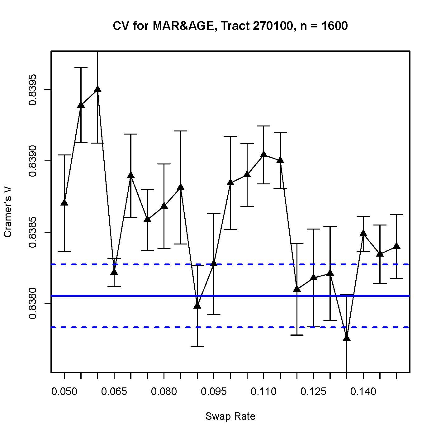
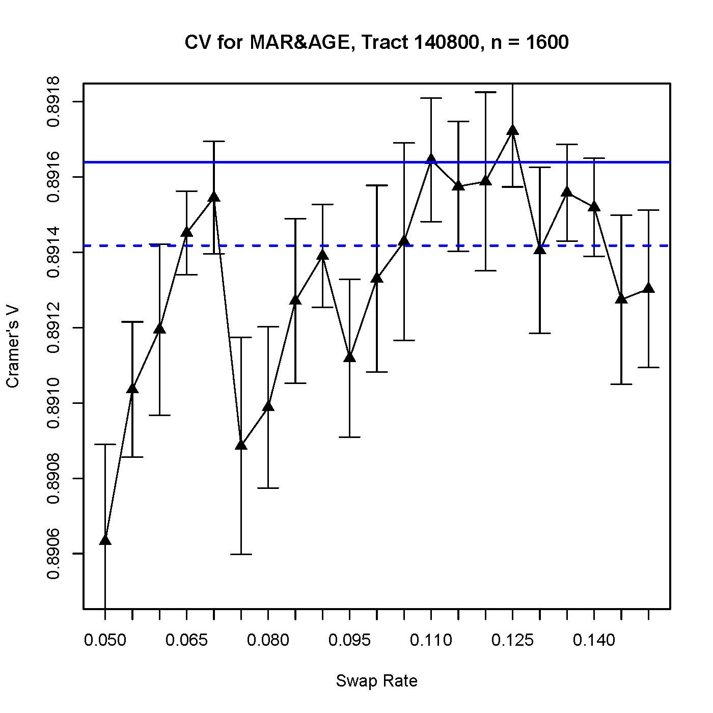
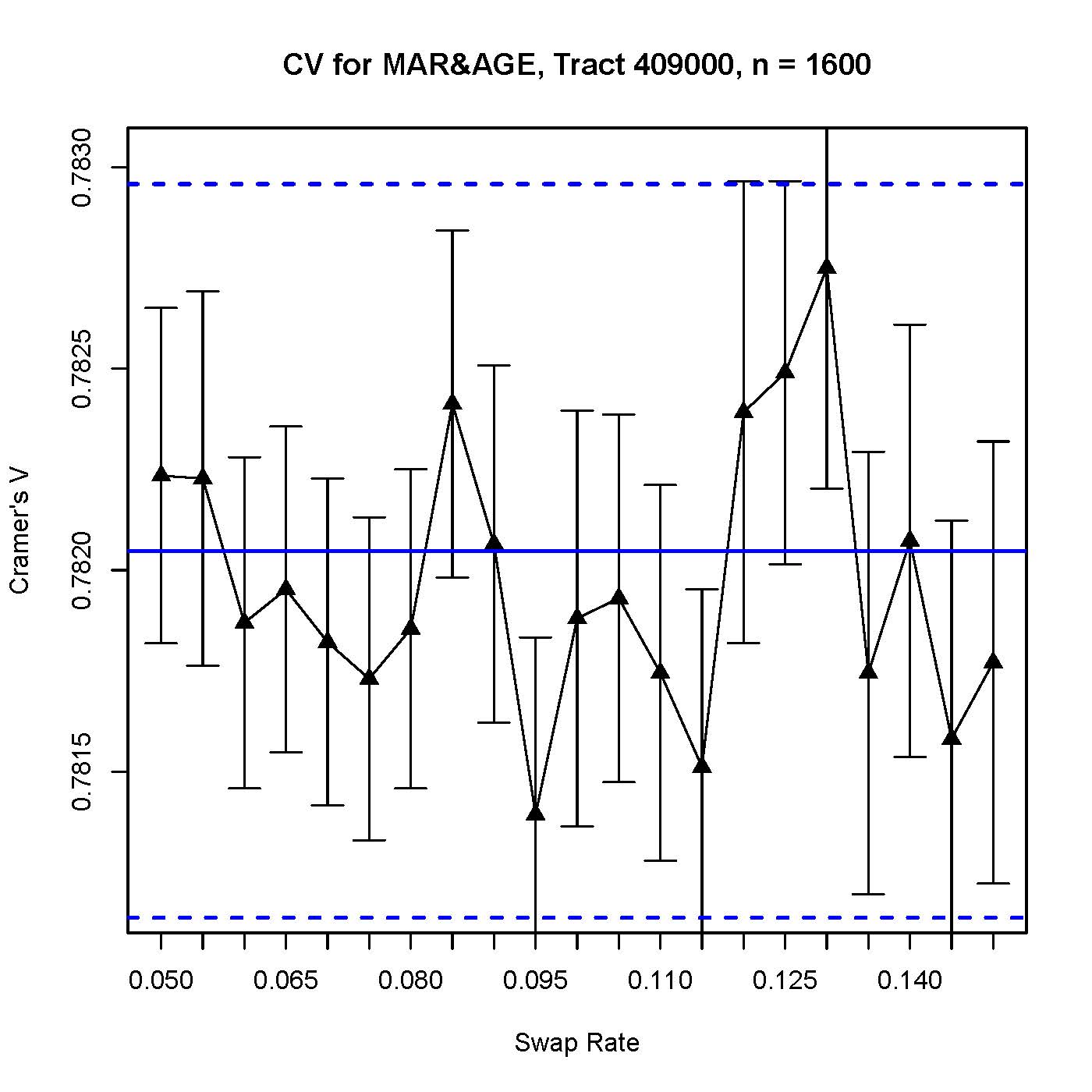
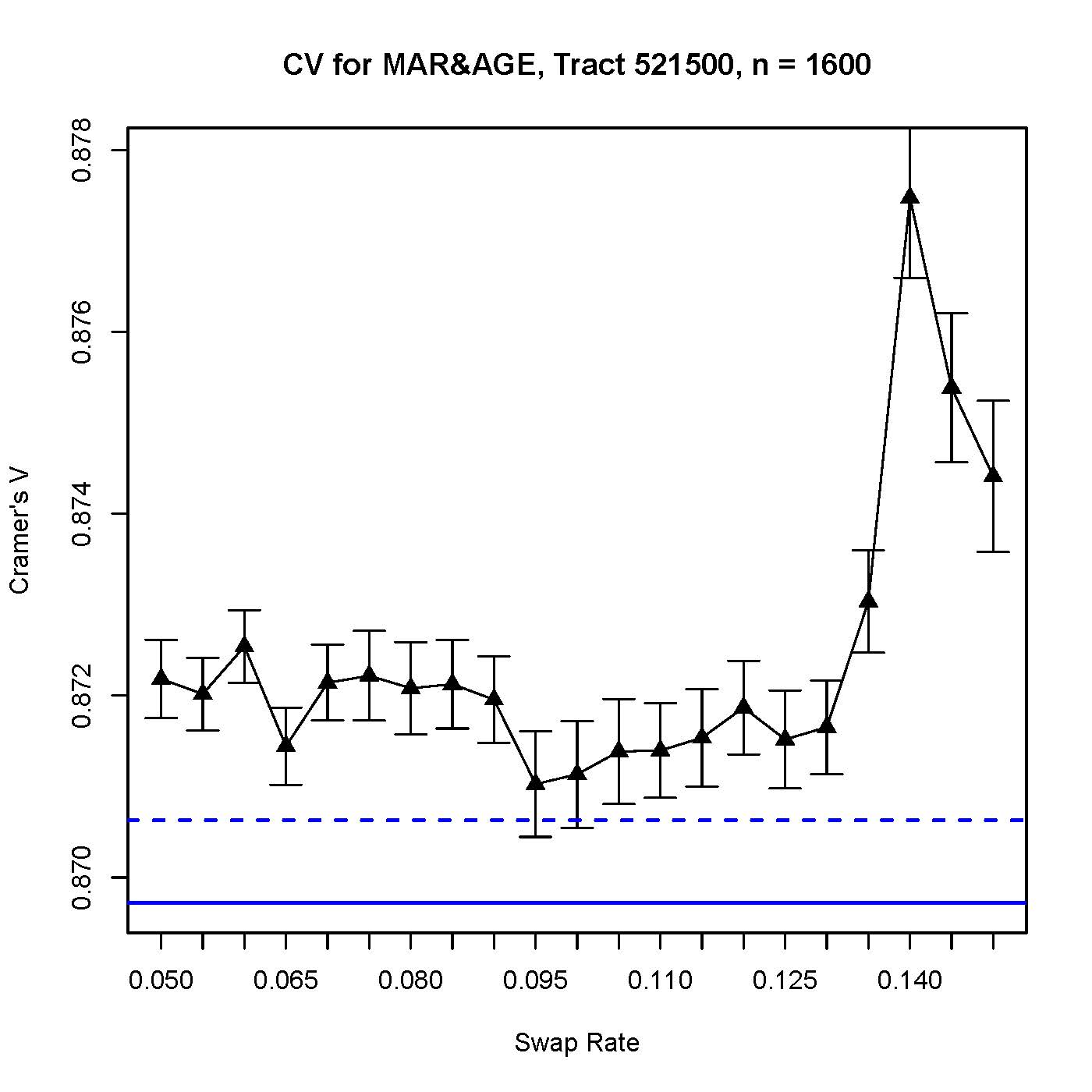
Figure 6: Cramér’s $V$ versus swap rates for the tables of marital status by age (very sparse but strong association).

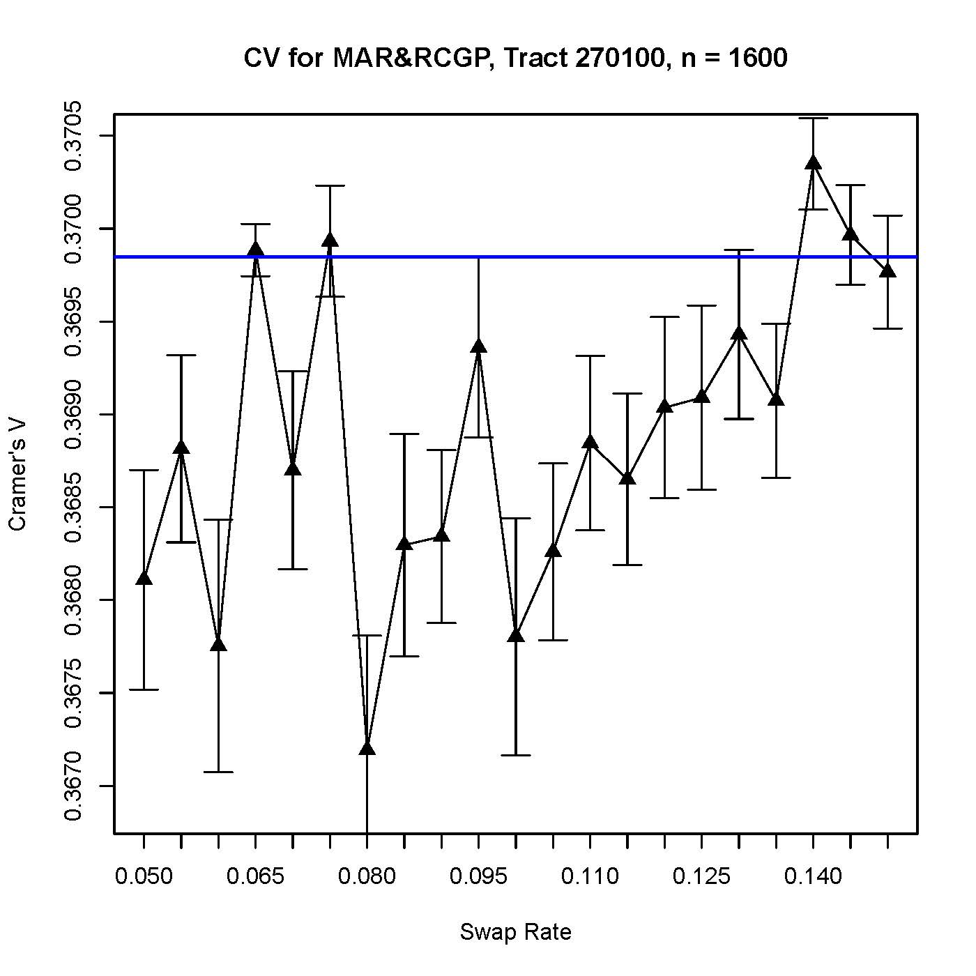
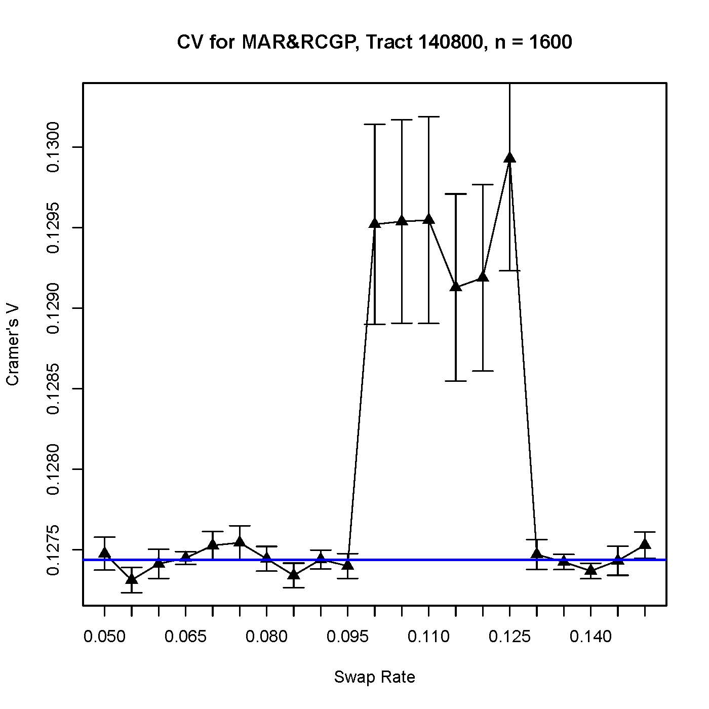
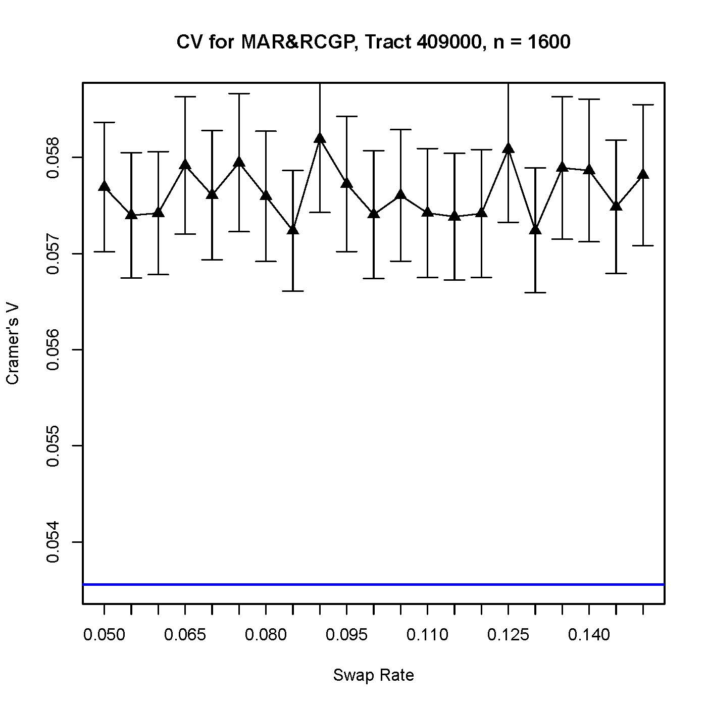
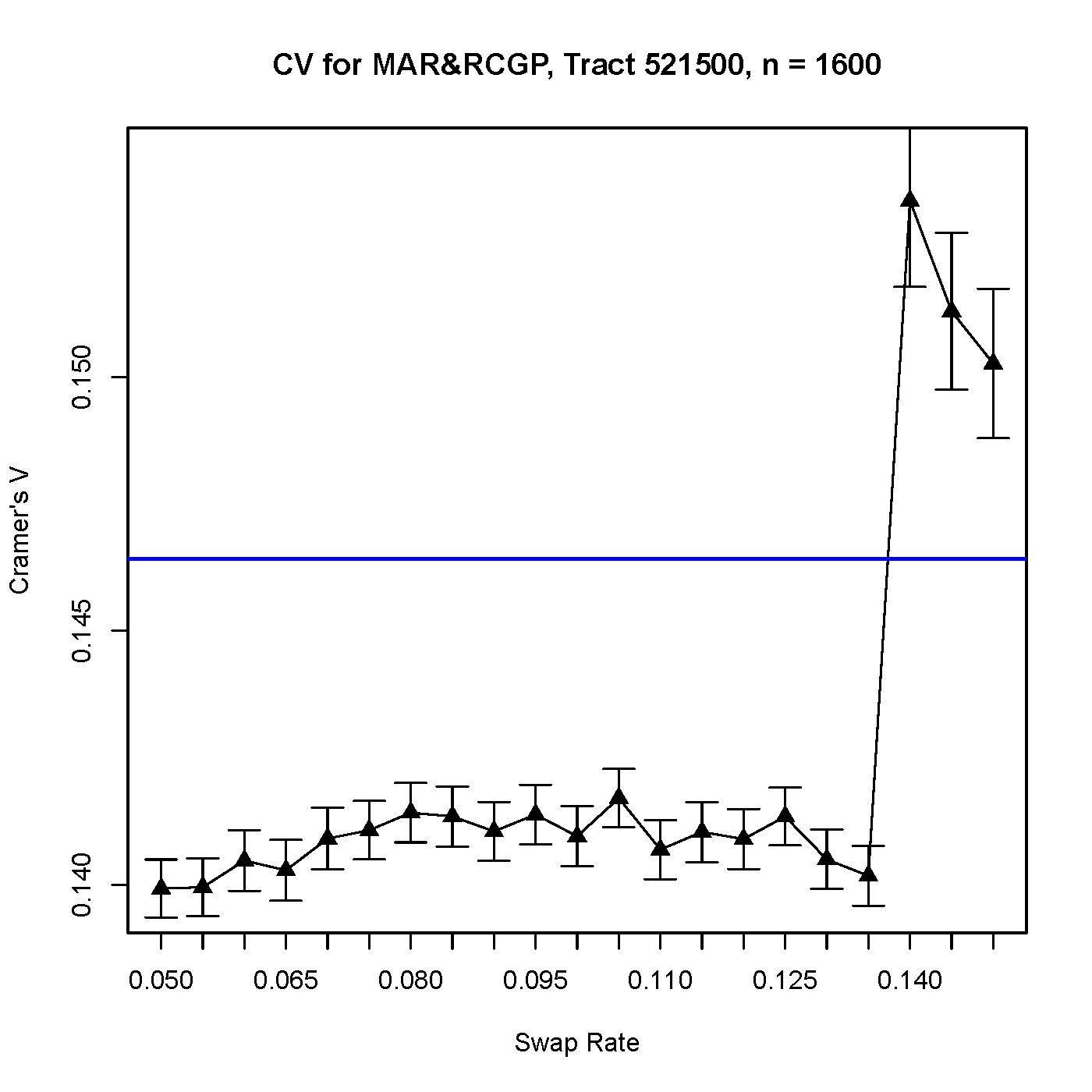
Figure 7: Cramér’s $V$ versus swap rates for the tables of marital status by race (not sparse, but weaker association).

4 Discussion

Data swapping in its simplest form, wherein a fraction of households is swapped at random, will “normalize” the strengths of the joint distributions of categorical variables, instead of lowering them. This effect is still observed even when a primitive matching stage is included, so that two households may only be swapped if they match on some predefined set of key variables. However, the further addition of a minimal targeting stage in the data swapping procedure is shown to impact the statistical quality of the data in an inconsistent way: by deciding to implement a generic selection criterium for at-risk households, even the expected direction of swapping’s effect on the joint distributions can no longer be predicted.

The goal of this simulation study was to understand the impact of data swapping on statistical analyses of U.S. Census data. One way this work only approximates this goal is that the specifics of this data swapping algorithm cannot perfectly match what the Census Bureau has, since the true details of that algorithm are hidden from the public. Inspiration was drawn from what is publicly known about the true data swapping method, but these results are only a step towards the right direction. The targeting stage of the algorithm would be a natural focus for a future analysis; it may be that a different choice of at-risk variables used for selecting the set of records to swap may lessen the effect noticed in this paper, at least for a particular set of variables whose joint distributions are of particular interest.

Another point of interest is in expanding the list of statistical measures considered their susceptibility to data swapping’s effects. Cramér’s $V$ was merely chosen due to its similarity to the ubiquitous Pearson’s chi-square, but many other measures and statistical procedures are of interest to researchers across fields. In particular, an analysis of more robust measures of association than Pearson’s chi-square (and by extension, Cramér’s $V$) would be of use in separating the effect of data swapping and data sparsity. In this analysis, collapsing variables served as a stand-in for a more robust measure whenever the data were deemed to be too sparse. A follow-up study may better capture the true effects of data swapping by considering a non-asymptotic statistic.

The $n$-Cycle swap procedure is based on the idea of data swapping, except groups of $n$ individuals are chosen simultaneously and their records are permuted. In other words, data swapping is $n$-Cycling in the case where $n=2$; the procedure and its benefits are explained in detail in an article by DePersio et al. (2012). Some extension of the approach outlined in this paper may be useful for understanding the effect of $n$-Cycling on statistical measures. The process of evaluating the distortions to statistical analyses should be updated in this time when researchers have ever-increasing access to public census data and computational resources.

References

- Alexander et al. (2010) J. Trent Alexander, Michael Davern, and Betsey Stevenson. The Polls–Review: Inaccurate Age and Sex Data in the Census Pums Files: Evidence and Implications. Public Opinion Quarterly, 74(3):551–569, 2010. doi: 10.1093/poq/nfq033. URL http://poq.oxfordjournals.org/content/74/3/551.abstract.
- Carlson and Salabasis (2002) Michael Carlson and Mickael Salabasis. A data-swapping technique using ranks – a method for disclosure control. Research in Official Statistics, (2):35–64, 2002.
- Crimi and Eddy (2014) Nicole Crimi and William F. Eddy. Top-Coding and Public Use Microdata Samples from the U.S. Census Bureau. Journal of Privacy and Confidentiality, 6(2):21–58, 2014.
- DePersio et al. (2012) Michael DePersio, Marlow Lemons, Kaleli A. Ramanayake, Julie Tsay, and Laura Zayatz. n-Cycle Swapping for the American Community Survey. In Josep Domingo-Ferrer and Ilenia Tinnirello, editors, Privacy in Statistical Databases, volume 7556 of Lecture Notes in Computer Science, pages 143–164. Springer Berlin Heidelberg, 2012. ISBN 978-3-642-33626-3. doi: 10.1007/978-3-642-33627-0˙12. URL http://dx.doi.org/10.1007/978-3-642-33627-0_12.
- Fienberg and McIntyre (2005) Stephen E. Fienberg and Julie McIntyre. Data Swapping: Variations on a Theme by Dalenius and Reiss. Journal of Official Statistics, 21(2):309–323, 2005.
- Griffin et al. (1989) Richard A. Griffin, Alfred Navarro, and Linda Flores-Baez. Disclosure Avoidance for the 1990 Census. Proceedings of the Section on Survey Research, pages 516–521, 1989.
- Hawala (2003) Sam Hawala. Microdata Disclosure Protection – Research and Experiences at the US Census Bureau. Workshop on Microdata, Stockholm Sweden, August 2003.
- Lemons (2014) Marlow Lemons. Predictive Modeling of Uniform Differential Item Functioning Preservation Likelihoods After Applying Disclosure Avoidance Techniques to Protect Privacy. PhD thesis, Virginia Polytechnic Institute and State University, Blacksburg, Virginia, March 2014.
- Lemons et al. (2015) Marlow Lemons, Aref Dajani, and Jiashen You. Measuring the degree of difference in perturbed data. In JSM Proceedings, Alexandria, VA, 2015. American Statistical Association.
- Shlomo et al. (2011) Natalie Shlomo, Caroline Tudor, and Paul Groom. Privacy in Statistical Databases, volume 6344, chapter Data Swapping for Protecting Census Tables, pages 41–51. Springer Berlin Heidelberg, 2011.
- Zayatz et al. (1996) Laura Zayatz, Richard Moore, and B. Timothy Evans. New Directions in Disclosure Limitation at the Census Bureau. Technical Report LVZ96/01, US Bureau of the Census, 1996.
- Zayatz et al. (2010) Laura Zayatz, Jason Lucero, Paul Massell, and Asoka Ramanayake. Disclosure avoidance for Census 2010 and American Community Survey five-year tabular data products. In Section on Survey Research Methods - JSM 2010, pages 2279–2288, Alexandria, VA, 2010. American Statistical Association.