Lightning Strikes and Attribution of Climatic Change

Abstract

Using lightning strikes as an example, two possible schemes are discussed for the attribution of changes in event frequency to climate change, and estimating the cost associated with them. The schemes determine the fraction of events that should be attributed to climatic change, and the fraction that should be attributed to natural chance. They both allow for the expected increase in claims and the fluctuations about this expected value. Importantly, the attribution fraction proposed in the second of these schemes is necessarily different to that found in epidemiological studies. This ensures that the statistically expected fraction of attributed claims is correctly equal to the expected increase in claims. The analysis of lightning data highlights two particular difficulties with data-driven, as opposed to modeled, attribution studies. The first is the possibility of unknown “confounding” variables that can influence the strike frequency. This is partly accounted for here by considering the influence of temperature changes within a given month, so as to standardise the data to allow for cyclical climatic influences. The second is the possibility suggested by the data presented here, that climate change may lead to qualitatively different climate patterns, with a different relationship between e.g. strike frequency and temperature.

I Introduction

Lightning strikes and the damage caused by them are generally expected to increase as global temperatures rise Mills ; Williams ; Price1 ; Price2 ; Price3 ; Michalon ; Toumi ; Romps . The mechanisms behind this are being determined Williams ; Romps , and despite changes in strike-frequency being dependent on geographical location, the observed trend is very clear Mills ; Williams ; Price1 ; Price2 ; Price3 ; Michalon ; Toumi ; Romps . Consequently, lightning strikes provide an example where the statistical connection between insurance claims, lightning strikes, and temperature changes is increasingly well understood. A well known example is the Hartford Insurance Co. lightning strike data presented in Ref. Mills , that shows a very strong correlation between claim frequency and temperature. However, it is difficult to determine whether the relationship between number of claims and temperature is a causal one, with an increased temperature causing an increased number of strikes (and claims), or a co-incidental correlation, with lightning strikes tending to occur during the summer period for example. This is one of the questions that are considered here, as we explore the effectiveness of this and similar data, for lightning-strike attribution studies.

Presuming that a quantitative relationship can be determined between climate change (through the proxy of temperature in this example), and strike frequency, then in principle it becomes possible for changes in the number (and cost) of insurance claims, to be paid for by the polluter through a carbon tax CTax0 ; CTax1 ; NYTimes or an insurance-led levy WebsterClarke ; Clarke . For this to happen an additional difficulty needs to be overcome - to devise a mechanism that fairly attributes (e.g.) insurance claim costs between climatic change and natural statistical chance Pielke ; Otto ; Hannant . This is considered in Section III.

In section II we will consider lightning strikes across the contiguous United States, and the extent to which monthly-averaged data such as that presented in Ref. Mills can be used for attributing changes in lightning strike frequency to climate change. This raises two interesting concerns for data-driven studies. The first is the influence of “confounding” variables that are not included in the study, but also influence e.g. strike frequency. The second is the possibility of qualitative changes in climate patterns making data-driven climate models unreliable. Section III considers two schemes for splitting the number of strikes so that one fraction is attributed to climate change and the other to natural statistical chance. The lightning strike data is used to give an example of the proposed attribution schemes in Section V, estimating the number of strikes that should be attributed to climate change.

II Lightning strikes

Figure 1: The average number of lightning strikes per month in the United States is plotted (vertical axis), versus the area-weighted yearly-averaged temperature. The first data point is for 1996 in the top left of the plot, the last is for 2014 near the bottom of the plot, and adjacent years are connected by a dashed line. The majority of points for 1996-2011 are clustered around 60-75 strikes per month at a temperature of 52-54 degrees Fahrenheit, but the last three years 2012-2014 appear to be separated from the group. We do not know whether this is due to changes in reporting, or if it indicates a qualitative change in climate behaviour.

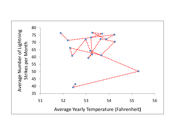
Here we reconsider the relationship between reported lightning strike damage and monthly averaged U.S. temperatures reported in Ref. Mills , using an enlarged database from 1996-2014, provided by the National Climatic Data Centre (NCDC). The temperature data is from the GHCN monthly climate indices for the area-weighted average temperature of the contiguous United States Menne . The lightning strike data is from the National Centre for Environmental Information’s Storm Events Database, that records lightning strikes that result in personal injuries and damage. In principle this includes strikes in Alaska, the Gulf of Mexico, Hawaii, and Hawaii waters, but these are comparatively small in number, and can be neglected when compared to the numbers recorded for the contiguous United States. We start by using this data to compare the average monthly strike rate and the year-averaged temperature (figure 1). Most of the data is grouped around 60-80 strikes per month with yearly-averaged temperatures of 52-54 degrees Fahrenheit, but the last 3 years 2012-2014 are clearly separated from this group. We do not know whether this is due to changes in the reporting of lightning strike events, whether it reflects a solar or other natural climatic cycle, or whether it is a symptom of a qualitative change in the climate. A straight line fit to figure 1 determines an increase in strike frequency that equates to approximately 2.9% per degree Celcius, or 3.0% per degree Celcius if the last three years 2012-2014 are omitted. These estimates are lower than the estimate of 12$\pm$5% per degree Celcius reported recently Romps , but not necessarily inconsistent with it. For example, if the strike frequency increases faster than linearly with temperature then the average number of strikes is likely to be greater than the number of strikes expected at the average temperature (or in mathematical notation $E[N(T)]\geq N(E[T])$, which is Jensen’s inequality Jensen ). In practice this means that if the expected strike rate is calculated with measurements that are averaged over shorter monthly time-scales, then we expect to find a higher estimate than that from figure 1. (In mathematical notation, if we sum over the months $i$ from $1$ to $12$ then provided $N(T)$ is a convex function, then, $(1/12)\sum_{i=1}^{12}N(T_{i})\geq N((1/12)\sum_{i=1}^{12}T_{i}$, and the total number of strikes in a year has $\sum_{i=1}^{12}N(T_{i})\geq 12\times N((1/12)\sum_{i=1}^{12}T_{i})$) This is one simple way in which an estimate based on yearly averages can be too low, others are discussed later, but it is related to a more serious concern that is discussed next.

Figure 2: For all years 1996-2014, the number of lightning strikes in a month is plotted (vertical axis), versus the average monthly temperature (horizontal axis). There is an approximately exponential increase in the rate of strikes with temperature. However September is clearly hotter than April, but there are generally less strikes in September, indicating that temperature cannot be the only variable that influences the number of strikes.

Figure 3: The average number of lightning strikes in a month January-December (vertical axis), is plotted versus the average monthly temperature (horizontal axis). January is the leftmost data point, July is top-right, and December is bottom-left, with adjacent months connected by a dashed line. There is a clear cyclical behaviour, indicating that initially the number of strikes increases more rapidly than temperature, and then subsequently falls more rapidly than temperature.

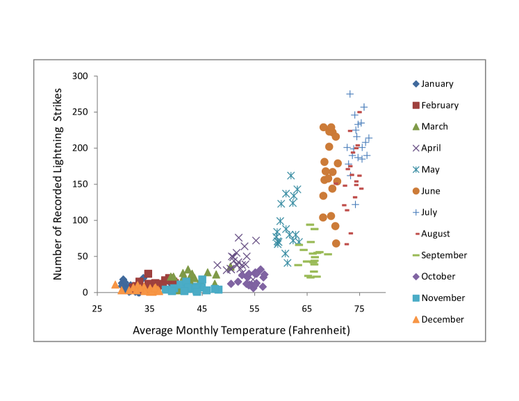
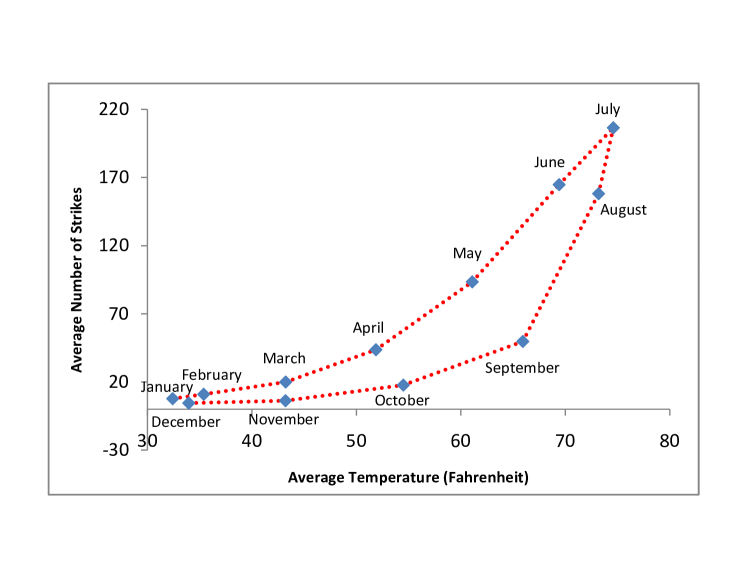
The Hartford Insurance Co. data Mills suggests a strong almost exponential relationship between the number of strikes and temperature. However, how can we be sure that the change in strikes is due to changes in temperature, and not a coincidence, with the conditions when strikes are more common being by chance at times of year when the temperature is hotter? To explore this possibility we plot the number of strikes versus average monthly temperatures, but grouped so that we know which strikes arise from a given month. If you compare April with September for example, it is clear that September has a higher average temperature than April, but the typical number of strikes is lower. The conclusion is that temperature is not the sole factor determining rate of strikes, there are other climate factors that must also be accounted for. This becomes particularly clear if we plot the average number of strikes in a given month versus the average temperature of that month (figure 3). This shows a clear cyclical behaviour with a higher rate of strikes at a given temperature in the spring than in the autumn. The cyclical plot is because the rate of increase in strike rate early in the year is faster than increases in temperature, and the rate of reduction in strike rate later in the year is slower than the rate of reduction in temperature. One interpretation is that the lightning strike rate has a more immediate response to an increase in heat (energy) being input into the climate system, whereas the temperature is slower to respond due to the large thermal inertia (specific heat capacity) of water and land mass.

To help separate the influence of other possibly cyclical climatic factors on strike rate from the influence of temperature, as far as is possible with monthly-averaged data sets, we consider the relationship between strike rate and temperature within each individual month. This approach is analogous to separating car drivers into different age groups when trying to assess the influence of wearing glasses on accident risk - older drivers are more likely to wear glasses than younger drivers, recording drivers age groups helps to standardise EpiUn the data so that the influence of age is separated from the influence of wearing glasses. The data available for each month is only 1/12 of that from the entire year, which increases the statistical variability of the data. Nonetheless, to make quantitative statements about the probability of events we would like a probability density function (“pdf”) for the monthly data for average temperature and number of strikes. A simple Bivariate probability density function (pdf) is used to fit the pairs of monthly data points $(N_{i},T_{i})$, with,

$$P(N,T)=\frac{1}{2\pi\sigma_{N}\sigma_{T}}\frac{1}{\sqrt{1-\rho^{2}}}\exp\left\{-\frac{\left[\left(\frac{N-\mu_{N}}{\sigma_{N}}\right)^{2}+\left(\frac{T-\mu_{T}}{\sigma_{T}}\right)^{2}-2\rho\left(\frac{N-\mu_{N}}{\sigma_{N}}\right)\left(\frac{T-\mu_{T}}{\sigma_{T}}\right)\right]}{2\left(1-\rho^{2}\right)}\right\}$$ (1)

The parameters $\mu_{N}$, $\mu_{T}$, $\sigma_{N}$, $\sigma_{T}$, and $\rho$, are here determined with a maximum-likelihood best fit Jensen . The Bivariate pdf is a generalisation of the normal distribution to two variables, and allows for a correlation between $N$ and $T$, that is quantified by $\rho$. This gives a probability density function (pdf) for $N$ and $T$, $P(N,T)$.

The Bivariate fit to the monthly data provides a pdf for pairs of $(N,T)$, but we would like to know the pdf for the number of strikes given the temperature, $P(N|T)$. Probability theory Jaynes requires that $P(N,T)=P(N|T)P(T)$, allowing us to obtain $P(N|T)$ from $P(N|T)=P(N,T)/P(T)$. If we approximate the pdf $P(T)$ for the (monthly-averaged) temperature of a given month with a Normal distribution, then we can solve for $P(N|T)$ in terms of the fitting parameters for $P(N,T)$, with,

$$P(N|T)=\frac{1}{\sqrt{2\pi}}\frac{1}{\sigma_{N}\sqrt{1-\rho^{2}}}\exp\left\{-\frac{1}{2}\frac{1}{\sigma_{N}^{2}(1-\rho^{2})}\left[N-\left(\bar{N}-\rho\bar{T}\frac{\sigma_{N}}{\sigma_{T}}\right)-\rho\frac{\sigma_{N}}{\sigma_{T}}T\right]^{2}\right\}$$ (2)

Because $N$ and $T$ are averages (over a month), the choice of Bivariate and Normal pdfs are suggested by the central limit theorem Jaynes , that with reasonable mathematical assumptions, requires the pdf for an average to have a Normal distribution (or Bivariate when generalised to two variables). Notice the form of the expression within the square brackets of Eq. 2, of $[N-a-bT]$, with

$$a=\bar{N}-\rho\bar{T}\frac{\sigma_{N}}{\sigma_{T}}$$ (3)

and

$$b=\rho\frac{\sigma_{N}}{\sigma_{T}}$$ (4)

The values of $a$ and $b$ are equivalent to those that would be obtained from a least squares best fit for $N(T)$, but now we additionally have an estimate for the standard deviation of $\sigma_{N}(1-\rho^{2})$, and more importantly a pdf for $P(N|T)$. The value of b determines how the expected number of claims will increase with temperature in a given month. If we average $b$ over all the months, we obtain an estimate of a 5.6% increase in claims per degree C.

It is not surprising that the monthly-averaged estimate is different to the yearly-averaged one discussed in Section II. Using the example discussed in Section II, if the relationship between strike rate and temperature were convex then an increased estimate is what we would expect from Jensen’s inequality Jensen , and the estimate would be expected to be increased further if we used weekly- or daily-averaged data. However the situation is more complicated, as is discussed shortly. The estimate of 5.6% is made using recorded observations of lightning strikes on the ground, and is closer to the value of 12$\pm$5% estimated from satellite data and climate modeling in Ref. Romps than the estimate using the yearly-averaged data in figure 1.

According to the data, the change in strike rate with temperature varies considerably for different months. The largest increases in strike rate are for August (averaging 158 recorded strikes per month, but estimated to increase by 25% per degree Celcius), and May (averaging 93 recorded strikes per month, but estimated to increase by 13% per degree Celcius). In contrast, for June there is an expected decrease in strike rate (averaging 165 recorded strikes per month, with a -9% expected change in strike frequency per degree Celcius). July presently has the most recorded strikes (averaging 207 per month), and these are expected to increase by about 7% per degree Celcius.

The average monthly changes in temperature from those in the 20th century are not uniform either. The data used here gives the average increase in temperature during the period 1996-2014 (across the spatially averaged contiguous United States), as 0.67 degrees Celcius (1.21 degrees Fahrenheit), from those in the 20th century. However the increase in monthly temperatures are greatest for the months from November to March, with an average increase of 0.90 degrees Celcius (1.63 degrees Fahrenheit), but smaller for the months from April to September whose average increase is 0.53 degrees Celcius (0.90 degrees Fahrenheit). Consequently the change in strikes with temperature will not simply be 5.6% per degree Celcius, because the temperature changes expected in each individual month can be very different to the average across all months. An average increase in temperature by 0.67 degrees Celcius from the 20th century average would give an estimated increase in strikes of 0.67$\times$5.6=3.8%. In contrast, if we use the 20th century average monthly temperatures to estimate the equivalent number of strikes for 20th century climate, then we estimate a reduction in the average number of strikes per year from 784 during 1996-2014 to 758. This suggests that the number of strikes has increased by 3.4% since the 20th century (100$\times$25.7/758.1). This is slightly less than the 3.8% increase that was estimated using the average value of $b$ and the average change in temperature. It equates to a 5.1% increase in strikes per degree Celcius increase in average temperature. Because this latter estimate more accurately accounts for non-uniform changes in monthly temperatures, in principle it would be expected to be more accurate than estimates using the average monthly response (average $b$), to an average change in temperature.

The average yearly standard deviation in the number of strikes can be estimated from $\sum_{i=1}^{12}\sigma_{N}(i)\sqrt{1-\rho^{2}(i)}$, where $\sigma_{N}(i)$ is the standard deviation of the number of strikes in the $i$th month, and $\rho(i)$ is the correlation coefficient for the $i$th month. Normalising this by the total average yearly number of strikes gives an estimated variation of 29%, which is considerably higher than the expected increase in temperature per degree, independent of whether an estimate of 5.6% or 5.1% are used.

III Attribution of climate change

The climate is only statistically predictable. The average expected temperature can be predicted, but the specific temperature cannot. Consequently the average number of claims due to climate change are in principle predictable, but not the actual number. Therefore if a carbon tax for example were used to pay for the increase in claims, then an immediate question is whether it should contribute to the expected increase in claims, or the actual number that is observed? Two options that we will explore in more detail shortly are:

• Pay a predetermined rate as a carbon tax CTax0 ; CTax1 ; NYTimes or insurance levy WebsterClarke ; Clarke , possibly annually, that is based upon the expected number of claims.

• Pay for a fraction of the total claims that actually occur, with that fraction determined in a way that reflects the relative likelihood for that number of claims occurring in the presence (and absence) of climate change.

The advantage of (B) is that the actual number of claims made are subsidised, so the insurance industry does not profit in good years, and is fully compensated in bad years. The disadvantage of (B) is that the subsidy paid to the insurance industry (and claimed from e.g. carbon emitting industries), will fluctuate in response to the natural statistical variability of the climate. Similarly, a disadvantage of (A) is that the subsidy paid or received (some claims might reduce due to climate change), would only on average be expected to match the actual changes in claim size; although the uncertainty in the average change in claim size can be estimated. An option (C) is to “split the difference”, so that half the costs are paid by method (A) and half by method (B), with the advantages and disadvantages shared by both the insurance industry and whoever is paying the subsidy. In practice this might involve the payer of the subsidy paying extra to insure themselves against such cost increases. This suggests a simpler alternative that is similar to (A), whereby the subsidy payer pays an additional premium to acknowledge that the burden of uncertainty has been passed to the insurance companies. This situation is virtually equivalent to (C), but would operate like a simple modification of (A), and is the simplest scheme that captures the consequences of both the expected increase in claims and the extra costs due to fluctuations of the actual claim sizes. The simplicity of this is attractive, but it does require the insurance industry to be able to absorb any large fluctuations of the claim sizes from their expected values, whereas with scheme (B) the costs would be spread more broadly across both the insurance industry and those contributing to a carbon tax CTax0 ; CTax1 ; NYTimes (or insurance levy WebsterClarke ; Clarke ).

IV Attribution pricing mechanisms

Two simple attribution pricing mechanisms for schemes (A) and (B) are described next. The main purpose is to show that simple, pragmatic, pricing schemes can be formulated, and to highlight some of their properties, and some properties required of them. A variety of alternative pricing schemes could no-doubt be proposed. For simplicity we discuss the total number of claims made, as opposed to their total value, but the approach is easily modified.

Scheme (A)

Let $P(N|T)$ be the probability of $N$ claims given a change in temperature from $T_{0}$ to $T$, with $T_{0}$ corresponding to the 20th century average temperature for a particular month for example. With greater generality we could have used atmospheric carbon dioxide levels in place of temperature $T$, but for clarity temperature is used here. Then we can write $P(N|T)$ as,

$$P(N|T)=P(N|T_{0})+\left[P(N|T)-P(N|T_{0})\right]$$ (5)

which is an exact identity. Multiplying (5) by $N$ and integrating from $0$ to $\infty$ with respect to $N$, gives,

$$E\left[N|T\right]=E\left[N|T_{0}\right]+\delta E[N|T]$$ (6)

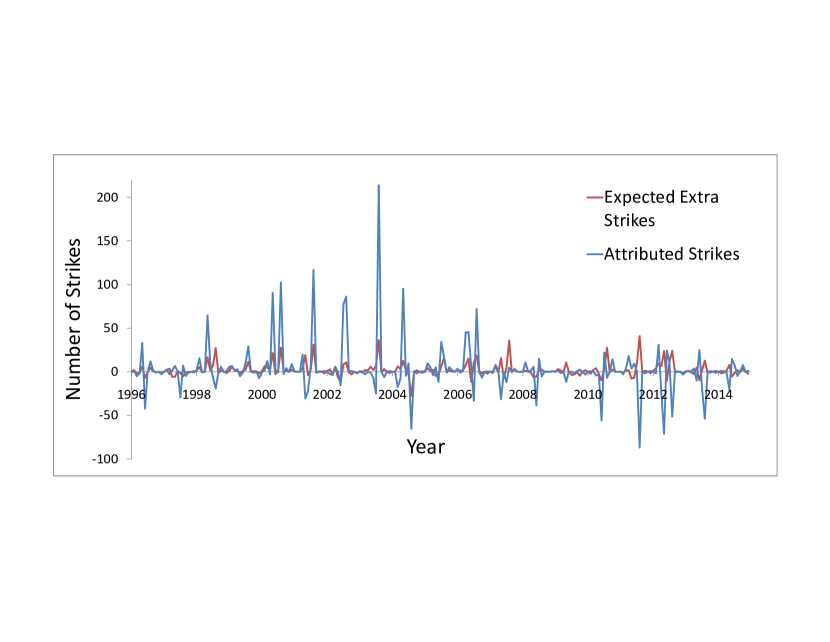
where the notation $E[N|T]$ denotes the expected value of N obtained by integration, and $\delta E[N|T]\equiv\int_{0}^{\infty}dN[NP(N|T)-NP(N|T_{0})]$ denotes the change in the expected number of claims due to a change in temperature from $T_{0}$ to $T$. In principle $\delta E[N|T]$ can be positive or negative, depending on whether $P(N|T)$ is greater or less than $P(N|T_{0})$, i.e. depending on whether climate change makes a claim more or less likely. An advantage of this simple approach is that $\delta E(N|T)$ can be calculated in advance using a climate model, and the estimate would then be determined in advance and would not fluctuate, unlike the actually observed values. The expected size of fluctuations about $\delta E(N|T)$ can also be estimated comparatively easily with varying degrees of sophistication. Alternatively, Eq. 6 can be used with the observed temperature data to give the expected number of extra strikes for the temperature $T$, compared with the expected temperature $T_{0}$ for that month, this is done later in figures 4-7. Note that depending on the values of $T$ and $T_{0}$, $\delta E[N|T]$ can be either positive or negative; it is possible that climate change can lead to less lightning strikes, certainly within individual months. Another advantage of this approach are its mathematical similarities to methodologies used in financial analysis, such as Modern Portfolio Theory (MPT) MPT and Credibility Theory Buhlmann , suggesting that it could easily be incorporated into financial models.

Scheme B

Scheme B requires that the total cost of actual claims that occur is paid partly from a carbon tax CTax0 ; CTax1 ; NYTimes or an insurance-led levy WebsterClarke ; Clarke , and partly by the individual insurance companies. This needs to be done fairly, and must recognise that statistically, any number of claims could in principle occur, independent of whether climate change happens or not. It also needs to recognise that statistically at least, climate change will modify the number of claims that are expected to occur, and it should be able to estimate the increased (or decreased) proportion of claims so that they can be correctly paid for by a carbon tax for example.

If we divide (5) by $P(N|T)$, and then multiply it by the observed number of claims $N$ then we have,

$$N=N\frac{P(N|T_{0})}{P(N|T)}+N\left(1-\frac{P(N|T_{0})}{P(N|T)}\right)$$ (7)

This equation (7) is exact, and has the property of splitting the claims so that $N=N\alpha+N(1-\alpha)$ with $\alpha=P(N|T_{0})/P(N|T)$. When the expected number of claims $N$ is independent of climate change with $P(N|T_{0})=P(N|T)$, then $\alpha=1$, a situation that would correspond to zero subsidy being paid. However if the expected number of claims has dramatically increased due to climate change, with $P(N|T)$ much larger than $P(N|T_{0})$, then $\alpha\rightarrow 0$, a situation corresponding to all the claims being paid for by a carbon tax (or insurance levy). The split between the payments is determined by $\alpha=P(N|T_{0})/P(N|T)$, that is determined by a quantitative model for the relative probability $\alpha$ of observing $N$ claims when climate change is, or is not, present. In the example here $P(N|T)$ is estimated from the observed data for lightning strikes, $T_{0}$ is the equivalent 20th century average monthly temperature, and $T$ is the observed monthly average temperature; but in principle there is no reason why a more sophisticated climate model should not be used. In principle $P(N|T)$ and $P(N|T_{0})$ can be determined from climate models, to give the relative probability of observing $N$ claims when climate change is, or is not, present. Actuaries will be familiar with the form of Eq. 7, because it is the same as the widely used credibility theory estimators Buhlmann . The fraction $(1-\alpha)=\left(P(N|T)-P(N|T_{0})\right)/P(N|T)$ will also be familiar to epidemiologists, because it is very similar to the “excess fraction” ModEp of extra incidences that result from exposure to new climate conditions. This latter point suggests that similar schemes could be used for other applications, such as quantifying the contribution an individual may have to a team’s performance for example. A difference between $(1-\alpha)$ and the excess fraction used in epidemiological studies, is that here the ratio $\alpha=(P(N|T_{0})/P(N|T)$ is the inverse to what would usually define an excess fraction in epidemiology EpiUn ; ModEp . This is deliberate and the reason why is explained below.

The excess fraction that we define considers $P(N|T_{0})/P(N|T)$, whereas the excess fraction used in epidemiological studies would consider $P(N|T)/P(N|T_{0})$ EpiUn ; ModEp . Why have we done this, and which is correct in this instance? On average, we would like the expected value of the attributed fraction of claims to equal the expected increase in claims as estimated by scheme (A). Therefore given the temperature and climate conditions and the probability density $P(N|T)$ associated with the temperature and climate conditions at the present (or future time), then we would like $E[N(1-\alpha)|T]$ to equal $E[N|T]-E[N|T_{0}]$. For the excess fraction that we define this is exactly the case,

$$\begin{array}[]{ll}E[N(1-\alpha)|T]&=\int_{0}^{\infty}N\left(1-\frac{P(N|T_{0})}{P(N|T)}\right)P(N|T)dN\\ &=E[N|T]-E[N|T_{0}]\end{array}$$ (8)

and the expected value of the fraction of claims attributed to climate change $N(1-\alpha)$, at the present or future climate conditions with temperature $T$, equals the expected increase in claims due to climate change. The requirement of $E[N(1-\alpha)]=E[N|T]-E[N|T_{0}]$ is the reason why the excess fraction that we have defined with $\alpha=P(N|T_{0})/P(N|T)$, is the correct one to use in this case, but is the inverse of the excess fraction usually used in epidemiology studies that would instead consider $P(N|T)/P(N|T_{0})$ EpiUn ; ModEp .

The separation of payments into those paid by the insurance company ($N\alpha$), and those paid by a climate change price ($N(1-\alpha)$), has all the properties we would want of a pricing scheme: i) Equation (7) is exact, there will be no over (or under) repayments in any given year, ii) The split in payments is determined in a quantitative way using probability theory, iii) The possibility that any given claim could statistically have occurred by chance is implicit, as is the recognition that the likely claim size can be modified by climate change, iv) Its expected value is the same as the expected increase in claims due to climate change, i.e. its average expected value is the same as scheme (A), v) It is simple to understand, and intuitively fair.

Figure 4: The attributed increase in lightning strikes compared to that expected for the 20th century are plotted (vertical axis), versus year (horizontal axis), for two attribution schemes (A) and (B). The expected increase in strikes (“Expected Extra Strikes”) are calculated from Eqs. 2 and 6, using the temperature data from 1996-2014 and the average 20th century temperature data. The number of strikes attributed to climate change using scheme (B) (“Attributed Strikes”), are calculated from $N(1-\alpha)$ with $\alpha=p(N|T_{0})/P(N|T)$ and using Eq. 2 with 1996-2014 and 20th century average monthly temperatures, and the observed numbers of strikes $N$. As expected, there are larger fluctuations with scheme (B) because they are proportional to the actually observed numbers of strikes. Because natural statistical variations can make the temperature less than 20th century averages, there are some years where the “Attributed” and “Expected” strikes are negative. As discussed in Figure 1, the years 2011-2014 have an unexpectedly low number lightning strikes.

Figure 5: Similarly to figure 4 the attributed increase in lightning strikes compared to that expected for the 20th century are plotted (vertical axis), but now versus each month in 1996-2014 (horizontal axis), for the two different attribution schemes (A) and (B).

V Example: Attribution of U.S. Lighting Strikes

As described in Section II, we estimate an average increase in strikes of 5.6% per degree Celcius, or 5.1% if the estimate compares the observed number of strikes during 1996-2014 with the estimated number of strikes for average 20th century monthly temperatures. We can estimate the cost of increased strike frequency by estimating the equivalent 20th century strike rate (estimated in Section II to be 758 strikes per year), and the damage cost estimates recorded in the NCDC storm events database that give an average cost per claim for the period 1996-2014 of $57800 (not adjusted for inflation). A 5.6% increase per degree corresponds to an estimated cost of $1.6M for the 0.67 degrees Celcius increase in average temperature in 1996-2014 above the average 20th century temperature. At the present estimated warming rate of 0.19 degree C per decade, in ten years the costs are estimated to rise to roughly $2.1M due to climate change (no adjustments for inflation in these estimates). If the estimate of a 5.1% increase in strikes per degree Celcius is used, then the estimated cost increases would become $1.5M for 1996-2014, increasing to $1.9M within ten years. Although the increase in (reported) costs are comparatively small compared with the US economy, they correspond to an increased strike frequency of approximately 4.8% and 4.4% (above those expected for 20th century temperatures).

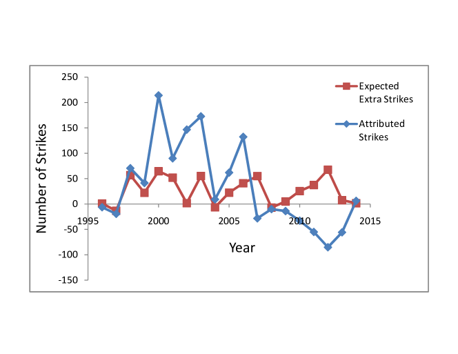
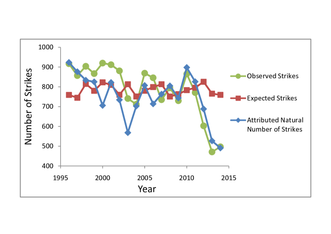
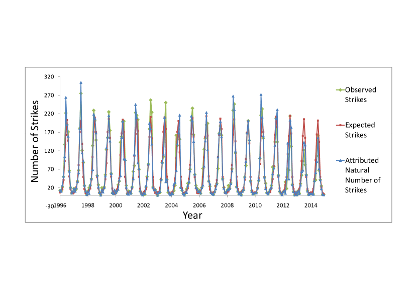
Section IV discussed two alternative attribution pricing mechanisms, scheme (A) that used the expected change in strike frequency, and scheme (B) that attributes a fraction of the total observed strikes to climate change. The number of strikes attributed to climate change is plotted for both methods in figures 4 and 5, that show the values averaged over a year and for individual months respectively. As expected, the variation in attributed numbers of strikes is greater for scheme (B) than for (A), which would make it more difficult to anticipate the costs using scheme (B). Another advantage of scheme (A) is that climate modeling could be used to estimate or define the expected number of attributed strikes in advance. However there are different benefits for scheme (B) over (A). Figures 6 and 7 plot the actual number of claims, and the number of naturally expected claims given the observed temperatures using schemes (A) and (B), averaged over a year and for individual months respectively. The oscillations seen in figure 7 are due to seasonal variations in climate and temperature over a yearly cycle. The advantage of scheme (B) is easiest to see from figure 6. Whereas the expected number of naturally occurring strikes remains comparatively stable, the attributed number of naturally expected strikes remains similar to the number of observed strikes. This helps to avoid subsidising claims that do not occur, and to ensure that if a large number of claims do occur, that they are fairly compensated. Arguably scheme (B) more accurately reflects the actual costs (or not), of climate change, but the costs are less predictable than for scheme (A). This is particularly true at present, because the natural yearly statistical variation in the number of strikes (estimated in Section II to be of order 29%), is much greater than the expected change in strike frequency due to climate change (the largest estimate here is a 5.6% increase in frequency).

The average number of strikes per year attributed to climate change during 1996-2014 by scheme A is 26, corresponding to a 3.4% increase compared with those expected for 20th century averages. This is equivalent to a 5.1% increase in strikes per degree Celcius, and is an identical calculation to the estimate in Section II that compared observed strike rates in 1996-2014 with those expected for 20th century temperatures. The average number of strikes per year in 1996-2014 that are attributed to climate change by scheme B is 34, corresponding to a 4.4% increase above the number expected for average 20th century temperatures. This equates to a 6.6% increase per degree Celcius. If the last three years 2012-2014 are excluded, scheme B would estimate that an average of 48 strikes per year should be attributed to climate change, a 6.4% increase, or 9.5% increase per degree Celcius. The estimates of scheme A remain fairly insensitive to whether the last three years 2012-2014 are included or not. The estimates reflect the qualitative remarks made earlier, with a greater volatility in estimates by scheme B than for scheme A. However scheme B more accurately reflects the number of strikes that actually occur. As discussed in Section IV, over a long enough time period, the estimates using schemes A and B will converge to the same average value.

Figure 6: The observed lightning strikes are plotted (vertical axis) versus year, along with the expected number of strikes as calculated using the observed temperature data and Eq. 2, and the number of strikes that would be attributed as “naturally” occurring ($N\times P(N|T_{0})/P(N|T))$. The different advantages of schemes (A) and (B) are clear - scheme (A) gives a less volatile estimate, but scheme (B) remains closer to the actually observed values.

Figure 7: Similarly to figure 6 the observed lightning strikes are plotted (vertical axis), but now versus month in years 1996-2014, along with the expected number of strikes as calculated using the observed temperature data and Eq. 2, and the number of strikes that would be attributed as “naturally” occurring ($N\times P(N|T_{0})/P(N|T))$. The monthly data clearly shows the periodic variation in frequency of lightning strikes through the year from winter to summer, with the majority of strikes occurring in the warmer spring and summer months.

VI Conclusions

Using monthly-averaged US temperature and lightning strike data as an example, we have considered two different schemes for determining how many lightning strikes should be attributed to climate change. Scheme (A) has the advantage of smaller fluctuations in the number of attributed strikes than scheme (B), but scheme (B) has the advantage of more accurately reflecting the actual number of observed strikes. Therefore, if a carbon tax CTax0 ; CTax1 ; NYTimes or insurance levy WebsterClarke ; Clarke were used to pay for the change in claim frequency (due to climate change), then scheme (B) would avoid over or under compensating claims attributed to climate change. The excess fraction used by scheme (B) uses a ratio $P(N|T_{0})/P(N|T)$ that is the inverse of what you would expect from analogous epidemiology studies. This is deliberate, and is shown to be necessary to ensure that the expected number of claims attributed to climate change will equal the expected change in the number of claims.

The recorded number of lightning strikes are not determined solely by the temperature but also have a clear seasonal dependence. To partially account for this, the dependence of lightning strikes on temperature was assessed within each individual month from January through to December. This led to an estimated average increase in claims per month of 5.6% per degree Celcius. It was also possible to use the monthly 20th century average temperatures to estimate how the number of strikes in 1996-2014 have increased from the 20th century average, finding a 5.1% increase per yearly-averaged temperature rise (in degrees Celcius). The increases are much less than the typical 29% variation in the observed number of strikes per year. If US temperatures continue to increase at 0.19 degrees Celcius per decade, then within ten years the estimates predict claims to increase from those expected for average 20th century temperatures by 4.8% and 4.4% respectively, with estimated increases in cost (for the claims reported in the NCDC storm events database), of roughly $2.1M and $1.9M (not adjusted for inflation). The lower estimate is the same as would be attributed to climate change by scheme A, and more comprehensively accounts for non-uniform changes in average monthly temperatures (as opposed to reporting a uniform average response), and therefore it seems likely to be a more accurate estimate. Scheme B attributes a 6.6% increase in strikes per degree Celcius to climate change, which is higher than scheme A, but over a sufficiently long time period estimates A and B will converge to the same value. All the estimates here are less than the estimate of 12$\pm$5% increase in strikes per increase in average temperature by one degree Celcius that is reported in Romps . The cause of this difference unclear. It could be caused by limitations in the data-driven analysis, such as the use of monthly-averaged data for example.

We end with a strong caveat originating from figure 1. Figure 1 suggests that there may have been a qualitative change in the climate in the past three years. It is possible that this is a naturally occurring change, or that it is due to a change in the reporting of strikes, in which case it does not reflect changes in climate and could be ignored. However, if it reflects a qualitative change in the climate then it is possible that the estimates here could become irrelevant for future studies. Because of Taylor’s theorem Arfken , a small linear response of (statistically averaged) climate properties would be expected in response to small changes in temperature, but if there is a strong non-linear response then data-based studies such as the one described here will become unreliable and climate modeling will be required. Nonetheless, studies such as the one here provide a useful baseline from which to compare future behaviour, and allow a discussion of how best to quantitatively estimate and attribute the cost of climate change.

Acknowledgments

Richard Clarke observed the exponential relationship between lightning strikes and temperature that triggered this work and stimulated a number of interesting discussions, some of which are expanded on in Refs. WebsterClarke ; Clarke . Thanks to Katie Webster for commenting on an earlier draft of this paper.

References

- (1) E. Mills , Science, 309, 1040, (2005).
- (2) E.R. Williams, Science, 256, 1184-1187, (1992).
- (3) C. Price, D. Rind, J. Geophys. Res., 97, 9919-9933, (1992).
- (4) C. Price, D. Rind, Mon. Weather Rev., 122, 1930-1939, (1994).
- (5) C. Price, D. Rind, J. Geophys. Res., 99, 10823, (1994).
- (6) N. Michalon, A. Nassif, T. Saori, J.F. Royer, C.A. Pontikis, Geophys. Res. Lett., 26, 3097-3100, (1999).
- (7) N. Reeve, R. Toumi, Q. J. R. Meteorol. Soc., 125, 893-903, (1999).
- (8) D.M. Romps, J.T. Seeley, D. Vollaro, J. Molinari, Science, 346, 851-854, (2014).
- (9) L.H. Goulder, Environmental Taxation and the “Double Dividend”: A Reader’s Guide, National Bureau of Economic Research (NBER), Working Paper # 4896, Oct, (1994).
- (10) G.E. Metcalf, D. Weisbach, The Design of a Carbon Tax, Harvard Environmental Law Review, 33, 2, 499-556, (2009).
- (11) New York Times, The Case for a Carbon Tax, http://nyti.ms/1FFvpZS, (2015).
- (12) A.J. Webster, R.H. Clarke, An Insurance-Led Response to Climate Change, submitted to Climatic Change, (2015).
- (13) R.H. Clarke, The Price of Carbon - A Market Led Approach for Tackling Climate Change, in preparation.
- (14) R.A. Pielke Jr. The Rightful Place of Science: Disasters and Climate Change, Arizona State University’s Consortium for Science, Policy, and Outcomes, ed. G.P. Zachary, Nov. (2014).
- (15) R. James, F. Otto, H. Parker, E. Boyd, R. Cornforth, D. Mitchell, M. Allen, Nature Climate Change, 4, 938, (2014).
- (16) A. Hannart, A. Carrassi, M. Bocquet, M. Ghil, P. Naveau, M. Pulido, J. Ruiz, P. Tandeo, DADA: Data assimilation for the detection and attribution of weather - and climate - related events, (submitted to Climatic Change), arXiv:1503.05236, (2015).
- (17) M.J. Menne, C.N. Williams Jr, R.S. Vose, Bull. Amer. Meteor. Soc., 90, 993–1007, (2009).
- (18) H. Hsu, Schaum’s Outline of Probability, Random Variables, and Random Processes, 2nd edition, The McGraw-Hill Companies Inc. (2011).
- (19) D. Coggon, G. Rose, D.J.P. Barker, Epidemiology for the Uninitiated, Fourth Ed., BMJ Publishing Group, (1997).
- (20) K.J. Rothman, S. Greenland, T.L. Lash, Modern Epidemiology, Third Edition, Lippincott Williams & Wilkins, Philadelphhia, USA. (2008).
- (21) E.T. Jaynes, Probability Theory the Logic of Science, (Cambridge University Press, (2003)).
- (22) E.J. Elton, M.J. Gruber, Journal of Banking & Finance, 21, 1743-1759, (1997).
- (23) H. Buhlmann, A. Gisler, A course in credibility theory and its applications, Springer, (2005).
- (24) G. Arfken, “Mathematical Methods for Physicists”, (San Diego, CA: Academic Press, (1985)).