Anisotropic singularities
in chiral modified gravity

Abstract

In four space-time dimensions, there exists a special infinite-parameter family of chiral modified gravity theories. All these theories describe just two propagating polarizations of the graviton. General Relativity with an arbitrary cosmological constant is the only parity-invariant member of this family. We review how these modified gravity theories arise within the framework of pure-connection formulation. We introduce a new convenient parametrisation of this family of theories by using certain set of auxiliary fields. Modifications of General Relativity can be arranged so as to become important in regions with large Weyl curvature, while the behaviour is indistinguishable from GR where Weyl curvature is small. We show how the Kasner singularity of General Relativity is resolved in a particular class of modified gravity theories of this type, leading to solutions in which the fundamental connection field is regular all through the space-time. There arises a new asymptotically De Sitter region ‘behind’ the would-be singularity, the complete solution thus being of a bounce type.

1 Introduction

We seem to live in four space-time dimensions, and so should take the structures available in this number of dimensions seriously. One of these is chirality. In the sense used here, this is related to Lorentz group having two different types of spinor representations. An object is called chiral if its spinor description uses more spinor indices of one type than of the other. In particular, self-dual 2-forms are chiral objects; see Appendix for a short review.

Chiral description of gravity

A remarkable phenomenon occurs in General Relativity (GR) in four space-time dimensions. This phenomenon is so stunning that we would like to refer to it as the chiral miracle. It is well-known to experts. Still, even after almost 40 years since its appearance in the literature, it has not become part of the background of all GR practitioners. This is why we start our discussion with a review of this phenomenon.

The miracle is related to a decomposition of the Riemann curvature. In view of its symmetries, the Riemann curvature $R_{\mu\nu\rho\sigma}$ can be thought of as a symmetric $\Lambda^{2}\otimes\Lambda^{2}$-valued matrix, where $\Lambda^{2}$ denotes the space of 2-forms. In four dimensions, we can decompose 2-forms into their self-dual and anti-self-dual parts $\Lambda^{2}=\Lambda^{+}\oplus\Lambda^{-}$, and so we have the decomposition of the Riemann curvature relative to the decomposition $\Lambda^{2}=\Lambda^{+}\oplus\Lambda^{-}$ :

$${\rm Riemann}=\left(\begin{array}[]{cc}A&B\vskip 3.0pt plus 1.0pt minus 1.0pt\\ B^{T}&C\end{array}\right)\,.$$ (1)

Here, $A$ and $C$ are symmetric $3\times 3$ matrices that can be referred to as the self-dual–self-dual and anti-self-dual–anti-self-dual parts of the Riemann curvature, respectively. For real metrics of Lorentzian signature, the matrix $C$ is the complex conjugate of $A$, and the matrix $B$ is a Hermitian $3\times 3$ matrix $(B^{T})^{*}=B$. The Bianchi identity $R_{[\mu\nu\rho\sigma]}=0$ implies that the traces of $A$ and $C$ are equal. In particular, for real Lorentzian metrics, this implies that the trace is real.

The above decomposition turns out to encode the irreducible pieces of the Riemann curvature with respect to the Lorentz (or orthogonal in the case of Riemannian signature) group. The trace of $A$ or $C$ is the scalar curvature. The trace-free parts of $A$ and $C$ are the self-dual and anti-self-dual parts of the Weyl curvature, respectively. The matrix $B$ encodes the trace-free part of the Ricci curvature.

Now comes the key point. In view of the above decomposition of the Riemann tensor, the Einstein condition is equivalent to

$$R_{\mu\nu}=\Lambda g_{\mu\nu}\qquad\Leftrightarrow\qquad\left\{\begin{array}[]{rcl}B&=&0\,,\vskip 3.0pt plus 1.0pt minus 1.0pt\\ {\rm Tr}\,A&=&\Lambda\,.\end{array}\right.$$ (2)

This relation uses only the first row of the matrix in (1). One could, of course, use the second row equally well. Thus, to impose the four-dimensional Einstein condition, it is sufficient to have access just to half of the Riemann curvature. This is the chiral miracle occurring in four-dimensional GR.

It is sometimes erroneously thought that this phenomenon has to do with complexification. Indeed, imposing some equation on a complex-valued quantity is equivalent to imposing two equations on two real quantities — the real and imaginary parts. However, this is not what happens here. The best way to see this is to consider the Riemannian, or all-plus signature. Most of the things stated above still apply, except that the two factors in the decomposition $\Lambda^{2}=\Lambda^{+}\oplus\Lambda^{-}$ are no longer complex conjugates of each other, both now being real (the Hodge star now satisfies $*^{2}=1$, with eigenvalues $\pm 1$, so the eigenspaces are real). In this case, the matrices $A$, $B$, and $C$ in (1) are all real-valued, and $C$ is related to $A$ only by the trace condition ${\rm Tr}\,A={\rm Tr}\,C$ that still follows from the Bianchi identity. The Einstein condition is still encoded in this case as given in (2). This makes it very clear that the fact that the Einstein condition is encoded in half of the Riemann curvature has nothing to do with complexification, as it still holds in the case of Riemannian signature, where the decomposition is real.

Reflection on the meaning of (2) leads to the following important theorem:

Theorem 1 (Atiyah–Hitchin–Singer ’78).

Let $X$ be a 4-manifold with an Einstein metric. Then the induced connection on the bundle $\Lambda^{+}$ of self-dual 2-forms is self-dual. Conversely, if the induced connection on $\Lambda^{+}$ is self-dual, then the metric is Einstein.

Here, a connection is called self-dual if its curvature is self-dual as a 2-form. The above theorem was discussed in [1] for metrics of Riemannian signature, but it continues to hold equally well for Lorentzian metrics.

The above theorem is the basis of what can be called chiral descriptions of the four-dimensional GR. There are several related versions of these, to be reviewed in the main text. The main idea is that some chiral (hence, complex-valued in the case of Lorentzian signature) object is used for the description of geometry, instead of the real-valued non-chiral metric on which the usual description is based. As can be anticipated from the fact that only half of the Riemann curvature is needed, such chiral descriptions are more economical than the metric GR, which justifies interest in them.

Chiral modifications of GR

While the chiral miracle described above is certainly known to differential geometers specialising in Einstein manifolds, there is another related miracle that is almost completely unknown to the community. It is the fact that the four-dimensional Einstein condition can be non-trivially deformed in a chiral way.

It is well known that GR can be modified, the simplest example of such a modification being the $R^{2}$ gravity, of relevance, e.g., as a good model of inflation [2, 3]. This model is equivalent to GR coupled to an additional scalar field, and so propagates not just the two polarisations of the graviton as in GR, but also a scalar. One can consider more involved modifications of GR with higher powers of the curvature added to the Lagrangian. One can quickly convince oneself that, because of the higher derivatives present in these modified theories, they all propagate more degrees of freedom (DOF) than does GR. If one insists on second-order field equations, then GR is the unique theory, at least in four dimensions. It thus seems impossible to modify GR without adding extra propagating DOF to it. This is the content of several GR uniqueness theorems available in the literature.

It then comes as a big surprise that it is indeed possible to modify GR without adding extra DOF if one starts from one of its chiral descriptions. The resulting chiral modified gravity theories continue to have second-order field equations. A complete count of the number of degrees of freedom by the Hamiltonian analysis shows that they have the same number of propagating degrees of freedom as in GR — the two propagating polarisation of the graviton. And, as will be reviewed below, there is an infinite-parametric class of such chiral modified gravity theories, in which GR is just a special member.

Once GR gets embedded into an infinitely large class of gravity theories all with similar properties, one is forced to ask a number of questions: What makes GR unique as compared to all these other theories? Why is the real world described so well by GR? Is it described by GR perfectly, or is this only an approximate truth? To put it differently, the very fact that such chiral modified gravity theories exist makes one obliged to understand them.

One, however, faces the following difficulty. In the chiral description of GR with Lorentzian signature, the metric ceases to be a fundamental field variable. One rather deals with a complex-valued field subject to appropriate ‘reality conditions’ to ensure the reality of the metric that this field defines. In GR, this procedure is (reasonably) well understood. In the case of chiral modifications of GR, the fundamental complex-valued field and the general structure of the theory remain intact; only the field dynamics gets modified continuously without appearance of new degrees of freedom. What remains much less understood, however, is how one is to modify the ‘reality conditions.’ Note that, since the metric is a derived field in the theory, it may no longer be required to remain real-valued in all cases in a chiral modification of GR. It appears that one cannot establish proper general ‘reality conditions’ before one considers coupling of gravity with matter, — the problem that lies beyond the scope of the present paper and still awaits for its solution.

Having said that, we should also remark that there are many situations where the chiral modified gravity theories behave perfectly sensibly and admit the usual interpretation in terms of a real-valued space-time metric. Moreover, one can also formulate these modified theories as theories of Riemannian signature metrics. In this case, all objects involved are real-valued, and the issues referred to above simply do not arise.

We should also stress that the type of modifications of gravity we are interested in here is unique in the following sense. One can inspect the proofs of the GR uniqueness, notably the modern proofs that deal with the scattering amplitudes, and note the particular assumptions in those proofs that are violated by our chiral theories. Removing those assumptions, one can see that there results a new ‘uniqueness’ theorem stating that these chiral modifications are the only ones that describe propagating gravitons with second-order field equations; see [4] for an argument of this sort.

All this encourages us to investigate these chiral modifications of GR in detail.

This paper

In this paper, as a step towards a better understanding of these modified gravity theories, we study them in a particular setup of Bianchi I space-times. Already in the case of GR, this is a rich setup, exhibiting the famous Kasner singular behaviour. The Kasner behaviour is widely expected to capture the essence of a generic spacelike singularity of General Relativity.

Our present work is related to earlier works by some of us [5, 6] (see also [7]), where the spherically symmetric problem was analysed. It was found that there is a peculiar mechanism that resolves the singularity inside a black hole in terms of the fundamental connection fields. Homogeneous and isotropic cosmological solutions in the modified gravity theory under investigation coincide with those of general relativity. The effects of modifications on the theory of cosmological perturbations were under investigation in [8].

Previous works on the physics of these modified gravity theories used a first-order formulation. The corresponding computations involved many auxiliary fields and were quite cumbersome. One of the aims of this paper is to put to use the recently developed and much more economical pure-connection formulation. As compared to previous works on the subject, this simplifies the analysis tremendously.

Our main result is that a generic class of modified gravity theories of the type studied here resolves the Kasner singularity of the GR solution of the Bianchi I model. This resolution occurs in a way similar to the case of black hole mentioned above: although the metric field based on this solution still contains singularities and experiences changes of signature, the fundamental connection field is everywhere regular.

To avoid misunderstanding, we would like to stress that in the family of modified gravity theories that we study modifications can be arranged so as to become important only in regions of large Weyl curvature. In the Bianchi I setup that we study this is the region near the would-be singularity. In regions of small Weyl curvature the modifications are negligible and these gravity theories behave indistinguishable from GR. To put it differently, the chiral modified gravity theories are continuously deformable to GR. So, by choosing the parameter(s) controlling the modification to be sufficiently small the modified theories will behave as GR on large scales, while exhibit behaviour very different from GR at small distances. The scale where modification becomes important can be chosen to be close to the Planck scale, and so one can view the setup that we study as a classical theory of gravity where gravity gets strongly modified close to the Planck scale, while remaining indistinguishable from GR at large distances.

New description of chiral modified gravity theories

Apart from direct application to Bianchi I models, this paper develops a new parametrisation of the underlying modified gravity theories. The new description uses not just a connection, but also a number of auxiliary fields assembled into a $3\times 3$ matrix. We refer to a description with auxiliary fields as ‘mixed’ in the main text, because it is half-way between the first-order formulation of the theory with even more fields, and the pure-connection formulation. The new mixed description turns out to be quite powerful. In particular, it allows for a description of GR with zero cosmological constant in an essentially pure-connection setting, something which is impossible if one works just with connections.

Although the new ‘mixed’ description of our modified gravity theories has been originally developed specifically for the present analysis of the Bianchi I setup, it later proved to be very powerful for a variety of other problems. Two recent papers [9] and [10], devoted to different issues, are substantially based upon this ‘mixed’ description.

Organisation of the paper

In Section 2, we describe the so-called pure-connection formulations of gravity. Modifications of gravity of the type studied in this paper are easiest to introduce in this pure-connection setup. We start with the Plebanski first-order description of GR. We then show how the chiral pure-connection formulation of GR arises, and motivate the modified theory as its certain generalisation. In this section, we also present the ‘mixed’ new parametrisation of the modified theory. In Section 3, we specialise to the sector of interest, which is that of Bianchi I connections. We introduce the evolution equations for the connection components and obtain the metric described by this connection. In Section 4, a convenient choice of the time variable is made, which allows us to solve the evolution equations for our theories in full generality, without making any assumption about the function that controls the modification. We also establish some general properties of the solution. Section 5 specialises to the case of GR with non-zero cosmological constant. We describe the connection components in this case, and obtain the Kasner behaviour of the metric, which is realised near the singularity. In Section 6, we analyse the solution in the case of a particular one-parameter family of modifications. It is here that we will see how the modification resolves the Kasner singularity. We end up with a discussion.

There is a number of appendices at the end of the paper. In the first Appendix, we review some basic facts about spinors and self-duality in four dimensions. The second Appendix starts with a more general assumption about the connections of interest, and derives the ansatz used in the main text. In the third Appendix, for completeness, we derive the GR solution working in physical (proper) time. This is possible, but is considerably more involved than the derivation presented in the main text. In the last Appendix, we derive the Bianchi I solution in GR with $\Lambda=0$ working in the ‘mixed’ parametrisation with auxiliary fields.

2 The pure-connection formulation(s) of gravity

One of the simplest ways to understand modifications of gravity of our type is to first formulate GR as a theory of connections. We will describe how this is done below. For now, let us just say that the connection plays the role of the potential for the metric, schematically $g=\partial A$, so that the metric is constructed from the first derivative of the connection. The gravity Lagrangian is constructed as an algebraic function of the curvature of the connection. A particular such function gives dynamics equivalent to that in GR, see below.

In the pure-connection formulation, GR can be straightforwardly modified by considering an arbitrary function of the curvature as the Lagrangian. This is guaranteed not to change the second-order character of field equations. Sometimes it also does not change the number of propagating degrees of freedom of the theory; see below.

At the very basic level, the way this approach works is as follows. There is some action principle with the only field appearing in the Lagrangian being the connection $A$. The arising Euler–Lagrange equations are second order partial differential equations for the connection, which schematically can be expressed as $\partial^{2}A=A$. For an arbitrary connection, not necessarily satisfying its field equations, one can construct a certain metric $g_{A}$ from (the first derivatives of) $A$. The Ricci tensor of $g_{A}$ is then of third order in derivatives of $A$. By using the connection field equations, $\partial^{2}A=A$, the Ricci tensor gets converted into an object of first order in derivatives of $A$. For the case of GR in this framework, this is just a multiple of the metric itself, and we obtain the vacuum Einstein equations. Thus, schematically,

$${\rm Ricci}[g_{A}]=\partial^{2}g_{A}=\partial^{3}A\underset{\hbox{\small on-shell}}{=}\partial A=g_{A}\,.$$ (3)

This explains how the field equations for the connection imply the Einstein equations for the metric $g_{A}$. Another similar line of identities can be written for the Weyl curvature of the metric $g_{A}$. In this case, the connection field equations imply that this Weyl curvature becomes (on-shell) identical to the curvature $F[A]$ of the connection itself:

$${\rm Weyl}[g_{A}]=\partial^{2}g_{A}=\partial^{3}A\underset{\hbox{\small on-shell}}{=}\partial A=F[A]\,.$$ (4)

The on-shell identification of the Weyl curvature with the curvature of $A$ makes it clear that an interesting class of modifications of gravity can be obtained in this formulation by simply appending the Lagrangian of GR with various scalars constructed from $F[A]$. These modifications will become important in regions where the Weyl curvature is large, and will thus have a chance to change the qualitative behaviour of solutions near anisotropic singularities. At the same time, such modifications of the Lagrangian for gravity do not lead to an increase in the order of field differential equations, which remain to be second-order partial differential equations for $A$.

The above discussion makes it clear that this approach to modifying GR is available in any ‘pure-connection’ formulation. There are several possible such formulations, as we shall now review. However, the above argument only guarantees that the order of field differential equations is unchanged, but it does not guarantee that the number of propagating degrees of freedom remains the same after modification. And indeed, the argument with scattering amplitudes [4] suggests that most of such modifications will introduce additional degrees of freedom.

After a brief review of the known pure-connection formulations, we will focus on the chiral pure-connection formulation, which is capable of modifying gravity without introducing new degrees of freedom.

2.1 Eddington–Schrödinger formulation

This is the pure-connection formulation of GR that is as old as the Einstein–Hilbert theory itself. As with all pure-connection formulations, a particularly simple way to get it is to start with the first-order formulation in which one has both the connection and the metric as independent variables. In the case of GR, this is the Palatini formulation, with the affine connection $\Gamma_{\mu\nu}{}^{\rho}$ and the metric $g_{\mu\nu}$. One then ‘integrates out’ the metric $g_{\mu\nu}$, i.e., solves the field equations for $g$ and substitutes the solution back into the action. This is only possible to do in the presence of a non-zero cosmological constant. As a result, an action principle is obtained that contains only $\Gamma_{\mu\nu}{}^{\rho}$. In the Eddington–Schrödinger case it is constructed from the (symmetric part of the) Ricci tensor

$$R_{\mu\nu}[\Gamma]:=R_{(\mu\alpha\nu)}{}^{\alpha}[\Gamma]\,,$$ (5)

where $R_{\mu\nu\rho}{}^{\sigma}[\Gamma]$ is the curvature of $\Gamma_{\mu\nu}{}^{\rho}$, the latter being assumed to be symmetric in its lower two indices. The pure-connection action principle is then

$$S[\Gamma]=\frac{1}{8\pi G\Lambda}\int\sqrt{{\rm det\,}\left(R_{\mu\nu}[\Gamma]\right)}\,d^{4}x\,.$$ (6)

It is not hard to check that the square root of the determinant of $R_{\mu\nu}[\Gamma]$ has the correct density weight so that the integral over the spacetime is well-defined.

The field equations that result from (6) are

$$\nabla_{\rho}R^{\mu\nu}[\Gamma]=0\,,$$ (7)

where $R^{\mu\nu}[\Gamma]$ is the inverse of $R_{\mu\nu}[\Gamma]$. If one now makes a definition

$$g_{\Gamma}:=\frac{1}{\Lambda}R_{\mu\nu}[\Gamma]\,,$$ (8)

then equation (7) tells that $\Gamma_{\mu\nu}{}^{\rho}$ is the $g_{\Gamma}$-compatible connection. The definition (8) of $g_{\Gamma}$ is then the vacuum Einstein equation.

The above description shows that this pure-connection formulation only makes sense when $\Lambda\not=0$. Another feature of this formulation is that the field equations (7) are highly non-polynomial in the derivatives of $\Gamma$, containing the inverse of $R_{\mu\nu}[\Gamma]$. Both these features are shared by any pure-connection description of gravity.

Theory (6) can be modified by considering more general functionals of $\Gamma$. For example, one can imagine dropping the symmetrization in (5) while keeping the same action (6). One can also take another contraction $R_{\mu\nu\alpha}{}^{\alpha}$ and form the same Eddington functional from it. More generally, any scalar density of weight one constructed from the Riemann tensor $R_{\mu\nu\rho}{}^{\sigma}(\Gamma)$ can serve as Lagrangian. It would be interesting to classify the freedom available here, and also to study the arising modifications. As we have already indicated above, it should be expected that modifications of the Eddington formalism will describe more degrees of freedom compared to those in GR.

2.2 The spin-connection formulation

To get this formulation, one proceeds in a similar way starting from a different first-order description. We can take it to be the Einstein–Cartan tetrad formulation. The trick of integrating out the vielbein from the first-order formulation can be carried out in $(2+1)$ dimensions [11]. This is best explained in Section 3.4 of [12]. Again, the nonzero cosmological constant is essential, and again one obtains a Lagrangian built from the square root of the determinant of the matrix of curvatures, which is characteristic of these approaches.

We are not aware of any pure spin-connection formulation in four spacetime dimensions. To obtain such a formulation, one would need to integrate out the tetrad, which in this case amounts to solving the equation

$$\epsilon^{IJKL}\theta^{J}\wedge F^{KL}[\omega]=\Lambda\epsilon^{IJKL}\theta^{J}\wedge\theta^{K}\wedge\theta^{L}\,,$$ (9)

where $\omega^{IJ}$ is the spin connection, $\theta^{I}$ is the tetrad, and the capital indices are the ‘internal’ four-dimensional ones. One would need to solve the above equation for the tetrad to obtain an algebraic function of the curvature $F^{IJ}_{\mu\nu}$. The pure-connection Lagrangian is then the determinant of the resulting tetrad. In contrast to all cases already considered where the solution presents itself readily, equation (9) is very non-trivial to solve, although it is not impossible that the corresponding pure-connection formulation does exist. It would be interesting to find it.

After the first version of the present manuscript has appeared on the arXiv, an interesting paper [13] appeared. In particular, this paper shows how (9) can be solved perturbatively, in terms of an expansion around a given background tetrad. The resulting pure-connection action has also been computed.

Another line of attack on this problem can be to replace the object $\theta^{I}\wedge\theta^{J}$ in the Einstein–Cartan Lagrangian by a 2-form object $B^{IJ}$. One can then add a term with a Lagrange multiplier field imposing the constraint that $B^{IJ}$ is of the type $\theta^{I}\wedge\theta^{J}$; see [14]. After that, one can integrate out $B^{IJ}$ as well as the Lagrange multiplier field, as we do later in the case of the chiral formulation. It would be interesting to perform this exercise and to compare the result with that of [13].

2.3 The chiral Plebanski formulation

In the chiral approach, one starts with the Plebanski formulation of GR [15] (see also [16, 17]). This is a first-order formulation, with an ${\mathfrak{s}u}(2)$ Lie-algebra-valued two-form field and a connection as independent variables. This formulation gives a concrete Lagrangian realisation of the Atiyah–Hitchin–Singer theorem reviewed in the Introduction. Let us start by describing this formulation, which is going to be the basis for all constructions in the present paper.

We denote the Lie-algebra indices by lower-case Latin letters $i,j,k,\ldots=1,2,3$. The basic fields are a Lie-algebra-valued two-form field with components $B^{i}$ and a connection one-form with components $A^{i}$. There is also a Lagrange multiplier field $\Psi^{ij}$, which is symmetric and traceless. The action of the theory is

$$S[B,A,\Psi]={\rm i}\int B^{i}\wedge F^{i}-\frac{1}{2}\left(\Psi^{ij}+\frac{\Lambda}{3}\delta^{ij}\right)B^{i}\wedge B^{j}\,.$$ (10)

Here, $\Lambda$ is the cosmological constant, which may be zero. The imaginary unit ${\rm i}=\sqrt{-1}$ in front of the action is needed in order to make it real for fields satisfying the reality conditions as appropriate for Lorentzian signature; see below. One would not need this pre-factor in either Riemannian or split signature.

Let us consider the field equations stemming from (10). First, varying with respect to $B^{i}$, we get

$$F^{i}=\left(\Psi^{ij}+\frac{\Lambda}{3}\delta^{ij}\right)B^{j}\,.$$ (11)

The Euler–Lagrange equation for the connection is

$$d_{A}B^{i}=0\,.$$ (12)

Finally, there is the equation obtained by varying with respect to $\Psi^{ij}$ :

$$B^{i}\wedge B^{j}\sim\delta^{ij}\,.$$ (13)

This equation can be understood as telling that $B^{i}$ ‘come from a tetrad’ in the sense that $B^{i}$ satisfying this equation contain no more information than that provided by the metric plus a choice of an ${\rm SO}(3)$ frame at every spacetime point. Equation (12) can be solved for $A^{i}$ in terms of derivatives of $B^{i}$ whenever $B^{i}$ are non-degenerate (that is, the three two-forms $B^{i}$ are linearly independent). In particular, equation (12) can be solved if the two-forms $B^{i}$ satisfy (13), in which case the solution $A^{i}$ can be shown to be just the self-dual part of the Levi-Civita connection for the metric described by $B^{i}$. Equation (11) then becomes a statement that the curvature of the self-dual part of the Levi-Civita connection of a metric is self-dual as a two-form. Atiyah-Hithich-Singer theorem stated in the Introduction guarantees this to be equivalent to the Einstein condition, which shows that (10) is indeed a description of GR. When all field equations are satisfied, i.e., on-shell, the field $\Psi^{ij}$ is identified with the self-dual part of the Weyl curvature. For more details on this formulation, the reader is referred, e.g., to [17].

2.4 The metric

In the above description, we have mentioned the fact that $B^{i}$ satisfying (13) contain no more information than that available in the metric (up to gauge rotations). This metric is determined by the two-form fields directly, as we now review.

The main point is the geometric idea that, in four dimensions, one knows the conformal class of the metric (i.e., the metric modulo multiplication by an arbitrary function) if one knows which two-forms are self-dual. Therefore, by declaring the triple of two-forms $B^{i}$ to be self-dual, one fixes the conformal class of the metric uniquely. Explicitly, the conformal class is given by the following representative due to Urbantke [18]:

$$g_{\mu\nu}\sqrt{{\rm det\,}g}\sim\tilde{\epsilon}^{\alpha\beta\gamma\delta}\epsilon^{ijk}B^{i}_{\mu\alpha}B^{j}_{\nu\beta}B^{k}_{\gamma\delta}\,.$$ (14)

Here $\tilde{\epsilon}^{\alpha\beta\gamma\delta}$ is the anti-symmetric tensor density of weight one which in any coordinate system has components $\pm 1$, and the proportionality means equality up to an arbitrary positive coordinate-dependent scalar factor. To fix the metric completely, it suffices to fix this factor, or to specify the associated volume form. In the case of the Plebanski theory that described GR, the associated volume form ${\mathcal{V}}$ is fixed uniquely from the requirement that the metric be Einstein. The correct volume form then turns out to be:

$$3!\,{\rm i}\,{\mathcal{V}}=B^{i}\wedge B^{i}\,.$$ (15)

The content of the previous subsection can then be summarised by saying that when field equations (11)–(13) are satisfied, the metric determined by (14) with the associated volume form determined by (15) is Einstein.

The above discussion applies to complexified GR, in which case all fields in the Plebanski Lagrangian are considered to be complex-valued. Different so-called ‘reality conditions’ are to be imposed to get different metric signatures. The easiest choice is the split signature, for which one simply takes all fields to be real. In terms of the gauge group, this corresponds to the real form ${\rm SL}(2,{\mathbb{R}})$ of ${\rm SL}(2,{\mathbb{C}})$. The Riemannian signature is obtained by taking the real form ${\rm SU}(2)$. Finally, to get the metrics of Lorentzian signature, one needs to work with complex-valued fields but impose the reality conditions (here and below, an overbar denotes complex conjugation)

$$B^{i}\wedge\bar{B}^{j}=0$$ (16)

together with the condition of reality of the volume form (15). The reality conditions (16) guarantee that the complex conjugate forms $\bar{B}^{i}$ are wedge product orthogonal to $B^{i}$. Given that we want to identify $B^{i}$ with self-dual two-forms, and self-dual two-forms are wedge product orthogonal to anti-self-dual ones, equation (16) is the correct reality condition because it simply states that anti-self-dual two-forms are complex conjugates of self-dual ones. In other words, the reality condition (16) guarantees that the conformal metric determined by (14) is real Lorentzian.

2.5 Modified Gravity

A particular family of modified gravity theories, inspired by the Plebanski formulation, was motivated and described in [19]. In one possible parametrisation, the modification is to allow the cosmological constant in (10) to be an arbitrary ${\rm SO}(3)$-invariant function of the field $\Psi^{ij}$ :

$$S[B,A,\Psi]={\rm i}\int B^{i}\wedge F^{i}-\frac{1}{2}\left(\Psi^{ij}+\frac{\Lambda(\Psi)}{3}\delta^{ij}\right)B^{i}\wedge B^{j}\,.$$ (17)

It can be shown [20] by the Hamiltonian analysis that this theory continues to propagate just two degrees of freedom, similarly to GR. At the same time, this is a modified theory of gravity, in which modification becomes important in spacetime regions where the function $\Lambda(\Psi)$ significantly deviates from a constant. A particularly simple one-parameter family of modifications is obtained by considering the function $\Lambda(\Psi)$ in the form of a quadratic polynomial in $\Psi^{ij}$ :

$$\Lambda(\Psi)=\Lambda_{0}-\frac{\alpha}{2}{\rm Tr\,}(\Psi^{2})\,,$$ (18)

where $\alpha$ is an arbitrary parameter with dimensions $L^{2}$ (i.e., inverse curvature). For this family of modified theories, one expects strong deviations from GR when the field $\Psi$ (encoding the Weyl curvature in GR) becomes of the order of $1/\alpha$.

Having specified the Lagrangian, we need to say something about the metric that these modified theories might describe. As in the case of unmodified Plebanski theory, one may declare the two-forms $B^{i}$ to be self-dual, which fixes the conformal class of the metric to be the Urbantke one (14). However, now there exist many different choices for the volume form. The most natural choice seems to be the one suggested by the pure-connection formulation, which is to be described below.

Lagrangian (17), with all fields taken complex-valued, describes modified complexified GR. For Riemannian and split signatures, one makes the same respective choice of reality conditions as in the unmodified Plebanski theory. Thus, in these signatures, the modified gravity theories under investigation have an honest existence. For Lorentzian signature, one might hope that choice (16) remains to be compatible with the dynamics of the theory after its modification. However, this is known to be not true in many situations. Thus, no general reality conditions are known at present that would allow for a physical interpretation of the modified theories (17). However, in some special situations, conditions (16), requiring the reality of the metric, are compatible with the dynamics. In these cases, one does obtain real metrics with Lorentzian signature as solutions to modified theories. These solutions exhibit interesting properties, and this is the reason why it looks justified to study them. Whether solutions of this kind can be imbedded into some future physical theory, to be defined by an appropriate generic choice of the reality conditions, is still an open problem.

The family of theories (17) was previously studied in [5, 6, 7, 8]. Due to a large number of independent field components present in (17), calculations with this theory are quite cumbersome. The pure-connection formulation introduced in [21] and [22] simplifies equations by eliminating most of the field components. It thus simplifies the study of these modified gravity theories considerably. The present paper is the first one where the effects of the modified gravity are analysed directly in the simpler pure-connection formulation.

2.6 An alternative parametrisation

As a step towards the pure-connection formulation, we now describe an equivalent, but slightly different parametrisation of the modified theories (17). Lagrangian (17) can be written as

$$S[B,A,M]={\rm i}\int B^{i}\wedge F^{i}-\frac{1}{2}M^{ij}B^{i}\wedge B^{j}\,,$$ (19)

where the symmetric nondegenerate matrix $M^{ij}$ is subject to the constraint

$${\rm Tr\,}M=\tilde{\Lambda}(M)\,.$$ (20)

Here, $\tilde{\Lambda}(M)$ is some ${\rm SO}(3)$-invariant function of the matrix $M$. It can be assumed without loss of generality that $\tilde{\Lambda}(M)$ only depends on the two invariants ${\rm Tr\,}(M^{2})$ and ${\rm Tr\,}(M^{3})$, because if it also depended on ${\rm Tr\,}M$, then the constraint equation (20) written in the form

$${\rm Tr\,}M=\tilde{\Lambda}\left({\rm Tr\,}M,{\rm Tr\,}(M^{2}),{\rm Tr\,}(M^{3})\right)$$ (21)

could be solved with respect to ${\rm Tr\,}M$, giving birth to a new equation of the form (21), in which a new function $\tilde{\Lambda}(M)$ would be (${\rm Tr\,}M$)-independent.

To make a link to the previous parametrisation, we introduce a new matrix variable $\Psi$ via the relation

$$\Psi^{ij}=M^{ij}-\frac{1}{3}\tilde{\Lambda}(M)\delta^{ij}\,.$$ (22)

This turns constraint (20) into the relation ${\rm Tr\,}\Psi=0$, and establishes equivalence between theories (19), (20) and (17) with $\Lambda(\Psi(M))=\tilde{\Lambda}(M)$. Because of this equivalence, we can identify $\Lambda(\Psi)$ and $\tilde{\Lambda}(M)$ and remove the tilde from the latter to simplify the notation.

2.7 The pure-connection formulation

The pure-connection formalism for GR, as well as for the modified theories (17), was developed in [21, 22]. Here, it will be instructive and useful to derive it from the first-order description (19), (20), which is equivalent to (17).

The pure-connection formulation of (17), or, alternatively, of (19), is obtained by integrating out all the fields apart from the connection. As the first step, one solves for the two-form fields:

$$B=M^{-1}F\,,$$ (23)

where $M^{-1}$ is the matrix inverse of $M^{ij}$. Substituting this back into (19), we obtain

$$S[A,M]=\frac{{\rm i}}{2}\int{\rm Tr\,}\left(M^{-1}F\wedge F\right)\,.$$ (24)

By choosing an arbitrary volume form ${\mathcal{V}}$, we define a matrix $X^{ij}$ of scalars related to the curvature wedge products as follows:

$$F^{i}\wedge F^{j}=X^{ij}{\mathcal{V}}\,.$$ (25)

The action then becomes

$$S[A,M]=\frac{{\rm i}}{2}\int{\rm Tr\,}\left(M^{-1}X\right){\mathcal{V}}\,.$$ (26)

Now we can integrate out the matrix $M$ by solving its (algebraic) field equation obtained by varying this action subject to constraint (20). This leads to the pure-connection action

$$S[A]=\frac{{\rm i}}{2}\int{\rm Tr\,}\left(M^{-1}(X)X\right){\mathcal{V}}\,.$$ (27)

This can alternatively be written as

$$S[A]=\frac{{\rm i}}{2}\int f(X){\mathcal{V}}\,,$$ (28)

which is the usual form of the pure-connection formulation as it is described, e.g., in [21]. From these expressions, we can identify the function $f(X)$ of the pure-connection formulation as

$$f(X)={\rm Tr\,}(M^{-1}(X)X)\,.$$ (29)

Since action (27) is stationary with respect to variations of $M$ [this gives the equation used to determine $M^{-1}(X)$], we also see that

$$\frac{\partial f}{\partial X}=M^{-1}(X)\,.$$ (30)

Thus, the only remaining unsolved field equation of (19),

$$d_{A}\left(M^{-1}(X)F\right)=0\,,$$ (31)

becomes the pure-connection formulation field equation

$$d_{A}\left(\frac{\partial f}{\partial X}F\right)=0\,.$$ (32)

This is a second-order partial differential equation for the connection.

Note that the SO(3)-invariant function $f(X)$ defined in (29) has an important property of being a homogeneous function of its argument: $f(zX)=zf(X)$ for any complex number $z$. This is because $X$ enters the action (26) linearly, so that the solution $M^{-1}(X)$ in (29) is invariant with respect to a rescaling of $X$. In view of this property, and using definition (25), we can express the Lagrangian in (28) symbolically as

$$f(X){\mathcal{V}}=f\left(F\wedge F\right)\,.$$ (33)

General Relativity (with a non-zero cosmological constant $\Lambda_{0}$) corresponds to a particular choice of the function $f(X)$ in (28); see [22]:

$$f_{\rm GR}(X)=\frac{1}{\Lambda_{0}}\left({\rm Tr\,}\sqrt{X}\right)^{2}\,.$$ (34)

Another choice of a homogeneous SO(3)-invariant function $f(X)$ gives modification of General Relativity. Such modifications can be regarded as GR with arbitrary function of the curvature $F$ added to the Lagrangian, as discussed above.

2.8 The metric from the connection

To clarify the statement that Lagrangian (34) describes GR, we should specify the metric $g$ that solves Einstein equations when $A$ satisfies its Euler-Lagrange equations. This can be done directly in the pure-connection language, without referring to the original Plebanski construction involving the two-form fields $B^{i}$.

As in the first-order Plebanski formalism, the metric is constructed in two steps. First, we notice that, when the field equations (23) are satisfied, the conformal class of metrics in which $B^{i}$ are self-dual is the same as the one in which $F^{i}$ are self-dual, since both sets of two-forms span the same three-dimensional subspace in the space of all two-forms. Thus, instead of using (14), we can obtain the conformal class of the metric directly from the curvature of the connection:

$$g_{\alpha\beta}\sqrt{{\rm det\,}g}\sim\tilde{\epsilon}^{\mu\nu\rho\sigma}\epsilon_{ijk}F^{i}_{\mu\nu}F^{j}_{\rho\alpha}F^{k}_{\sigma\beta}\,.$$ (35)

For complex-valued connection components $A^{i}$, the conformal class obtained is, in general, complex (i.e., does not contain any real-valued metric). The reality conditions that ensure that the conformal class is that of a real Lorentzian metric can be stated as

$$F^{i}\wedge\bar{F}^{j}=0\,.$$ (36)

All this parallels the above discussion; we have only replaced the two-forms $B^{i}$ by $F^{i}$.

In the second step, one specifies a particular metric in the conformal class already defined. To do so, it suffices to fix the associated volume form. The volume form ${\cal V}_{A}$ that gives the metric satisfying the Einstein equations in the case of theory (34) is determined by

$$-2{\rm i}\Lambda_{0}^{2}{\cal V}_{A}=\Lambda_{0}f_{\rm GR}(F\wedge F)\,.$$ (37)

The factor of the imaginary unit is needed in this relation for the same reason as in (28). Thus, in the case of pure-connection description of GR, the action of the theory (28) is just the total volume of the space, which is very appealing.

For a modified gravity theory with a general function $f\left(F\wedge F\right)$ as a Lagrangian, we do not yet know what the correct ‘physical’ metric would be. However, by analogy with GR, we could assume that the action is again the total volume calculated with respect to this metric. This would imply that the metric volume form is a multiple of $f\left(F\wedge F\right)$. It is this metric that we are going to study below.

2.9 Mixed parametrisation

It is not hard to pass from the Plebanski formulation of GR with $\Lambda\not=0$ to the pure-connection formulation of GR and to obtain the Lagrangian function (34). It turns out to be surprisingly hard, however, to characterise modifications even of a simple type (18) in the pure-connection language. It is also clear from (34) that the pure-connection description involves the operation of taking the square root of a matrix, which requires specifying its branch. Another issue with the pure-connection formulation is that it only makes sense for $\Lambda\not=0$.

To overcome these difficulties, in this subsection we introduce a new, ‘mixed’ parametrisation that lies half-way between the Plebanski first-order description (19) and the pure-connection description (28) and that combines the advantages of both. The idea is to avoid solving the field equations for $M$, and work with both $M$ and $A$ as independent variables.

Let us see how this can work in practice. As a first step, we replace the constrained variational problem for $M$ in (26) by an unconstrained one, with an additional Lagrange multiplier $\mu$ imposing the constraint:

$$S[A,M,\mu]=\frac{{\rm i}}{2}\int\left[{\rm Tr\,}\left(M^{-1}X\right)+\mu\left({\rm Tr\,}(M)-\Lambda(M)\right)\right]{\mathcal{V}}\,.$$ (38)

In the context of unmodified GR, the idea of using a Lagrange multiplier to impose the tracelessness constraint, to our knowledge, was first implemented in [23]. Variation with respect to $M$ then gives the equation

$$M^{-1}X=\mu\left(M-\frac{\partial\Lambda(M)}{\partial M}M\right)\,.$$ (39)

To get to the pure-connection formulation, we are supposed to solve this, and the constraint equation (20), for $M$ and $\mu$ in terms of $X$. However, this is very difficult to do in general. Only in the case of GR, where $\Lambda$ does not depend on $M$, one can do this and immediately obtain (34). For this reason, let us instead solve equation (39) with respect to $X$. Taking the trace of this equation, and using the constraint on $M$, as well as definition (29), we can eliminate the Lagrange multiplier $\mu$ and get

$$X=f(X)\frac{M^{2}-M\frac{\partial\Lambda(M)}{\partial M}M}{\Lambda(M)-{\rm Tr\,}\left[\frac{\partial\Lambda(M)}{\partial M}M\right]}\,.$$ (40)

Thus, the matrix $X$ is determined by $M$ up to scale. Then, if we interpret the field equation

$$d_{A}(M^{-1}F)=0$$ (41)

as a partial differential equation for $M$ and solve it, we will find $X$ from (40). This is the strategy we will follow below to solve the field equations in the case of homogeneous anisotropic cosmology.

Let us also give the form of relation (40) in the case of parametrisation by using variable (22) and function $\Lambda(\Psi)$ in (17). We have

$$X=f(X)\frac{\left(\Psi+\frac{1}{3}\Lambda(\Psi){\rm Id}\right)^{2}\left({\rm Id}-\frac{\partial\Lambda}{\partial\Psi}\right)}{\Lambda(\Psi)-{\rm Tr\,}\left(\frac{\partial\Lambda}{\partial\Psi}\Psi\right)}\,,$$ (42)

where Id denotes the identity matrix. In obtaining the above formula we have used the fact that the matrices $\Psi$ and $\partial\Lambda/\partial\Psi$ commute.

The case $\Lambda(\Psi)\equiv 0$, which corresponds to GR without the cosmological constant, needs to be considered separately. This theory does not have pure-connection formulation, but one can still solve the field equations in the mixed parametrisation proposed here. In this case, equation (39) gives

$$\Psi^{-1}X=\frac{1}{3}\Psi\,{\rm Tr\,}(\Psi^{-2}X)\,.$$ (43)

In particular, this equation implies that the function $f(X)={\rm Tr\,}(\Psi^{-1}(X)X)\equiv 0$ in the case of GR without the cosmological constant. We analyse the Bianchi I cosmology for this case in the Appendix.

In either of the two cases, one needs to solve the coupled system of equations (40), (41) or (43), (41) (with $M=\Psi$) and find the components of the connection. So, this is still a connection formulation with the connection playing the role of the main field. However, there are now additional auxiliary fields $\Psi$. One of the benefits of this mixed formulation is that, even in the case of GR, there is no need to take square roots. And, as we shall see below, the coupled system of equations can be solved, at least in special situations.

2.10 Gravitational Instantons

Before we proceed to the analysis of the homogeneous anisotropic field configurations as described by our modified gravity theories, we make one further remark about the gravitational instantons in our formalism. This subsection can be skipped on the first reading.

Let us rewrite the mixed parametrisation (38) of our theories as

$$S[A,M,\mu]=\frac{{\rm i}}{2}\int\left[{\rm Tr\,}\left(M^{-1}X\right)+\mu\,g(M)\right]{\mathcal{V}}\,,$$ (44)

where we have introduced a scalar-valued function of matrix $M$ :

$$g(M):={\rm Tr\,}M-\Lambda(M)\,.$$ (45)

The role of the Lagrange multiplier $\mu$ is to impose a single constraint on the matrix $M^{ij}$. This constraint can be viewed as defining a codimension-one surface $g(M)=0$ in the space of matrices $M$. By the Hamiltonian analysis of this class of theories, this constraint can be shown to be, in fact, the Hamiltonian constraint in disguise. As we have seen above, the function

$$g_{\rm GR}(M)={\rm Tr\,}M-\Lambda_{0}$$ (46)

with constant $\Lambda_{0}$ gives the description of GR with the cosmological constant $\Lambda_{0}$.

We now note that, $M$ being an auxiliary field, any field redefinition of $M$ in (44) should give an equivalent description of the theory. Thus, in particular, the Lagrangian

$$S[A,\tilde{M},\mu]=\frac{{\rm i}}{2}\int\left[{\rm Tr\,}\left(\tilde{M}X\right)+\mu\,\tilde{g}(\tilde{M})\right]{\mathcal{V}}\,,$$ (47)

where $\tilde{M}=M^{-1}$, and $\tilde{g}(\tilde{M})=g(\tilde{M}^{-1})$ should provide an equivalent description.

It is then interesting to note that, by taking

$$\tilde{g}_{\mbox{\scriptsize self-dual}}(\tilde{M})={\rm Tr\,}\tilde{M}-\Lambda_{0}$$ (48)

with constant $\Lambda_{0}$, one obtains a Lagrangian describing self-dual gravity. Indeed, varying (47) with respect to $\tilde{M}$, we obtain the equations

$$X^{ij}\sim\delta^{ij}\,,$$ (49)

which are known to provide the correct description of the gravitational instantons in the pure-connection formalism. In terms of the original action (44), this means choosing the function $g(M)$ in the form

$$g_{\mbox{\scriptsize self-dual}}(M)={\rm Tr\,}\left(M^{-1}\right)-\Lambda_{0}\,.$$ (50)

Thus, our mixed parametrisation is flexible enough to incorporate GR, modified gravity theories, and self-dual gravity. One just constraints the auxiliary matrix field onto different codimension-one surfaces. It is interesting that GR (46) and the instanton sector (50) go one into another by the replacement $M\to M^{-1}$ in the constraint equation.

3 Bianchi I connections

We now start exploring how the familiar general-relativistic Kasner solution arises in the above pure-connection formulation, and what the modifications of gravity entail.

The following ansatz for the Bianchi I connection is motivated in the Appendix:

$$A^{i}={\rm i}{h}_{i}(\tau)dx^{i}\,.$$ (51)

Note that there is no summation over $i$ on the right-hand-side of this equation. Here, ${h}_{i}(\tau)$ are three functions of an arbitrary time coordinate $\tau$, while $x^{i}$ are the Cartesian coordinates on the spatial slices (surfaces of homogeneity). The corresponding curvature two-form is

$$F^{i}=dA^{i}+\frac{1}{2}\epsilon^{ijk}A_{j}\wedge A_{k}={\rm i}\dot{h}_{i}d\tau\wedge dx^{i}-\frac{1}{2}\epsilon^{ijk}{h}_{j}{h}_{k}dx^{j}\wedge dx^{k}\,,$$ (52)

where an overdot denotes derivative with respect to $\tau$. Calculating the wedge product, we obtain

$$F^{i}\wedge F^{j}=-2{\rm i}\delta^{ij}X_{i}{h}{\cal V}_{c}\,,$$ (53)

where ${\cal V}_{c}=d\tau\wedge dx^{1}\wedge dx^{2}\wedge dx^{3}$ is the coordinate volume form, ${h}={h}_{1}{h}_{2}{h}_{3}$, and

$$X_{i}=\frac{\dot{h}_{i}}{{h}_{i}}\,.$$ (54)

If we select the volume form ${\cal V}$ in (25) to be

$${\cal V}=-2{\rm i}{h}{\cal V}_{c}\,,$$ (55)

then $X^{ij}={\rm diag}\,\left(X_{1},X_{2},X_{3}\right)$.

3.1 Evolution equations in the pure-connection parametrisation

The reason for the above choice of the volume form defining the matrix $X^{ij}$ is that the pure-connection formulation equation (32) reduces to the system

$$\left(\frac{\partial f}{\partial X_{i}}\right)^{\cdot}=f(X)-\frac{\partial f}{\partial X_{i}}\sum_{j}X_{j}\,,$$ (56)

which is a system of first-order differential equations for $X_{i}$. A derivation is given in the Appendix (in more generality), but, for the present situation with diagonal matrix $X$, it is quite easy to obtain these equations directly. Specialising to the case of the function $f(X)$ given by (34), it is not hard to obtain the familiar GR solution; see Appendix.

An alternative form of equations (56) is obtained by multiplying these equations by ${h}={h}_{1}{h}_{2}{h}_{3}$ and using definition (54). Equations (56) then reduce to

$$\left(\frac{\partial f}{\partial X_{i}}{h}\right)^{\cdot}=f(X){h}\,.$$ (57)

This form will be very convenient for analysing the case of arbitrary $f(X)$.

3.2 Evolution equations in the parametrisation with auxiliary fields

Let us also give the form of the evolution equations arising in the mixed parametrisation, which involves both the connection and the matrix $M$. The equation in question is then (41). Given that the matrix $M$ is the inverse of the matrix of first derivatives of the function $f(X)$ [see (30)], it is diagonal whenever $X$ is diagonal: $M^{ij}={\rm diag}(M_{1},M_{2},M_{3})$. Using relation (29), one can write equations (41) in a form similar to (57):

$$\left(M_{i}^{-1}{h}\right)^{\cdot}={\rm Tr\,}\left(M^{-1}X\right){h}\,.$$ (58)

This form will be most convenient for the analysis of modifications in the parametrisation by a function $\Lambda(\Psi)$.

3.3 The metric

Before we begin our analysis of the evolution equations given above, it is useful to compute the metric determined by the connection. To this end, one can follow the previously described procedure by first computing the Urbantke metric (35) and then conformally rescaling it so that the volume form becomes a multiple of $f\left(F\wedge F\right)$. A simpler method is to directly look for a metric that makes the curvature forms (52) self-dual.

We are looking for the metric in the Bianchi I form

$$ds^{2}=-N^{2}(\tau)d\tau^{2}+\sum_{i}a_{i}^{2}(\tau)\left(dx^{i}\right)^{2}\,.$$ (59)

Calculating the dual ${}^{*}F^{i}$ of the curvature two-forms (52) with respect to this metric, we have

$${}^{*}F^{i}=-{\rm i}\dot{h}_{i}\frac{Na_{1}a_{2}a_{3}}{2N^{2}a_{i}^{2}}\epsilon_{ijk}dx^{j}\wedge dx^{k}-\frac{1}{2}\epsilon^{ijk}{h}_{j}{h}_{k}\frac{Na_{1}a_{2}a_{3}}{a_{j}^{2}a_{k}^{2}}\epsilon_{jkl}d\tau\wedge dx^{l}\,.$$ (60)

The requirement ${}^{*}F^{i}={}\pm{\rm i}F^{i}$ gives the condition

$${}\pm\dot{h}_{1}=\frac{Na_{1}}{a_{2}a_{3}}{h}_{2}{h}_{3}\,,\quad\mbox{etc}\,,$$ (61)

from which we get

$$\frac{a_{1}^{2}}{N^{2}}=\frac{{h}_{1}^{2}}{X_{2}X_{3}}\,,\quad\mbox{etc}\,.$$ (62)

Another equation for determining the metric is obtained by fixing the metric volume form

$${\cal V}_{m}=Na_{1}a_{2}a_{3}d\tau\wedge dx^{1}\wedge dx^{2}\wedge dx^{3}=Na_{1}a_{2}a_{3}{\cal V}_{c}\,.$$ (63)

By our prescription, this should be equal to a multiple of $f\left(F\wedge F\right)$:

$$-2{\rm i}\Lambda_{0}{\cal V}_{m}=f\left(F\wedge F\right)\,,$$ (64)

where $\Lambda_{0}$ is some parameter of dimension $1/L^{2}$, later to be identified with the cosmological constant. Using (53), we get

$$\Lambda_{0}Na_{1}a_{2}a_{3}=f(X){h}\,.$$ (65)

Combining this equation with (62), we have

$$N^{2}=\left(\frac{f^{2}(X)\prod_{i}X_{i}^{2}}{\Lambda_{0}^{2}}\right)^{1/4}\,,\qquad a_{1}^{2}=N^{2}\frac{{h}_{1}^{2}}{X_{2}X_{3}}\,,\quad\mbox{etc}\,,$$ (66)

where the first relation is written in the form indicating that there are, in general, four possible branches, two of them imaginary. If we require that the metric be real, and that the signature of the $\tau$ coordinate be negative, then the final expression for the metric is

$$ds^{2}=\sqrt{\left|\frac{f(X)\prod_{i}X_{i}}{\Lambda_{0}}\right|}\left[-d\tau^{2}+\prod_{j}X_{j}^{-1}\sum_{k}{h}_{k}^{2}X_{k}\left(dx^{k}\right)^{2}\right]\,.$$ (67)

Note that this metric is time-reparametrisation invariant, as it should be.

4 Solution in the general case

One of the miracles of the pure-connection formulation of gravity under consideration is that it allows one to write the general solution to the problem at hand for an arbitrary theory, i.e., for an arbitrary choice of the function $f(X)$. This becomes possible by using a clever choice of the time variable.

We begin with solution for the case of general $f(X)$ and then specialise to GR and to a particular modified gravity theory. Solution of GR in which one works in the physical time from the beginning is also possible. For completeness, it is presented in the Appendix.

In the previous section, we arrived at evolution equations in the form (57). By using time-reparametrisation freedom, it is always possible to choose the time variable $\tau$ in such a way that

$$f{h}={\rm const}\,.$$ (68)

The geometric significance of this choice is that this is the time coordinate in which the metric volume form is proportional to the coordinate volume form, i.e., $\sqrt{{\rm det\,}g}=Na_{1}a_{2}a_{3}={\rm const}$. This is clear from (65).

With this choice, equation (57) can be integrated to give an implicit solution for $X(\tau)$:

$$\frac{\partial f(X)}{\partial X_{i}}=f(X)\left(\tau-\tau_{i}\right)\,,$$ (69)

where $\tau_{i}$ are arbitrary integration constants. The homogeneity of the function $f(X)$ implies another relation

$$\sum_{i}X_{i}\left(\tau-\tau_{i}\right)=1\,.$$ (70)

Equations (69) and (54) give a complete solution to the problem for an arbitrary theory from our class. We now give some general analysis of the solution obtained, and then consider some specific functions $f(X)$.

4.1 De Sitter solution

Consider $\tau\to\infty$, and assume that $f(X)\tau$ remains constant as $\tau\to\infty$. Then equation (69) implies that all derivatives $\partial f(X)/\partial X_{i}$ become mutually equal. The symmetry of the function $f(X)$, in turn, implies that all $X_{i}$ become equal to each other in this limit. Relation (70) then gives the solution

$$X_{i}\approx\frac{1}{3\tau}\quad\mbox{as \ $\tau\to\infty$}\,.$$ (71)

The homogeneity of $f(X)$ then justifies the assumption $f(X)\tau\to{\rm const}$ that we made in deriving this solution.

The corresponding metric describes the De Sitter spacetime. Indeed, we have $f(X)=f_{0}/\tau$, where $f_{0}$ is a constant. Then, by rescaling the spatial coordinates, we can always choose the solution in the form ${h}_{i}=\tau^{1/3}$. Then metric (67) becomes

$$ds^{2}=\sqrt{\frac{3f_{0}}{\Lambda_{0}}}\left(-\frac{d\tau^{2}}{9\tau^{2}}+\tau^{2/3}dr^{2}\right)=\sqrt{\frac{3f_{0}}{\Lambda_{0}}}\left(-dt^{2}+{\rm e}^{2t}dr^{2}\right)\,,$$ (72)

where $\tau={\rm e}^{3t}$ is the time coordinate change, and $dr^{2}=\sum_{i}\left(dx^{i}\right)^{2}$. This is nothing but the De Sitter metric, which is thus the solution of any modified theory.

4.2 Integration constants

Without loss of generality, one can shift the time variable so that

$$\sum_{i}\tau_{i}=0\,.$$ (73)

Second, apart from the trivial case $\tau_{i}=0$ for all $i$, which gives the De Sitter solution, by the remaining freedom of time rescaling, which does not violate (68), we can achieve the condition

$$\sum_{i}\tau_{i}^{2}=2\,.$$ (74)

This normalization is convenient because squaring (73) we can rewrite (74) as

$$\tau_{1}\tau_{2}+\tau_{2}\tau_{3}+\tau_{3}\tau_{1}=-1.$$ (75)

Without loss of generality, we can arrange the integration constants so that

$$\tau_{3}\leq\tau_{2}\leq\tau_{1}\,.$$ (76)

Because of condition (73), we have $\tau_{3}<0<\tau_{1}$. When $\tau_{2}=\tau_{1}$, we have $\tau_{2}=\tau_{1}=1/\sqrt{3}$ and $\tau_{3}=-2/\sqrt{3}$. This is the largest absolute value that $\tau_{3}$ can reach. In the opposite extreme $\tau_{2}=\tau_{3}$ we have $\tau_{2}=\tau_{3}=-1/\sqrt{3}$ and $\tau_{1}=2/\sqrt{3}$, which is the largest value $\tau_{1}$ can reach. All in all, we have

$$\tau_{c}\leq\tau_{1}\leq 2\tau_{c}\,,\qquad-\tau_{c}\leq\tau_{2}\leq\tau_{c}\,,\qquad-2\tau_{c}\leq\tau_{3}\leq-\tau_{c}\,,$$ (77)

where $\tau_{c}=1/\sqrt{3}$.

4.3 Solution in parametrisation with auxiliary matrix $M$

From now on, we will work in the mixed parametrisation with auxiliary matrix $M$. The evolution equation in this case takes the form (58). Choosing the same time variable as above, namely, the one that satisfies (68), we immediately obtain the solution

$$M^{-1}=f(X)T\,,$$ (78)

where $T^{ij}=\delta^{ij}(\tau-\tau_{i})$ is another diagonal matrix. This, in fact, is the same solution as (69); we simply refrained from solving the relation between $M$ and $X$. From this, we have

$${\rm Tr\,}M=\Lambda(M)=\frac{{\rm Tr\,}(T^{-1})}{f(X)}\,,\qquad M=\Lambda(M)\frac{T^{-1}}{{\rm Tr\,}(T^{-1})}\,.$$ (79)

Equation (40) then becomes

$$X=\frac{T^{-2}\left({\rm Id}-\frac{\partial\Lambda(M)}{\partial M}\right)}{{\rm Tr\,}\left[T^{-1}\left({\rm Id}-\frac{\partial\Lambda(M)}{\partial M}\right)\right]}\,.$$ (80)

The second equation in (79) enables one to find $M$ as a function of time. Substituting it into (80), one finds the solution for $X$.

4.4 Solution in parametrisation with auxiliary matrix $\Psi$

By expressing the partial derivatives in (80) in terms of $\Psi$ introduced in (22), one easily obtains a solution in the form

$$X=\frac{T^{-2}\left({\rm Id}-\frac{\partial\Lambda(\Psi)}{\partial\Psi}\right)}{{\rm Tr\,}\left[T^{-1}\left({\rm Id}-\frac{\partial\Lambda(\Psi)}{\partial\Psi}\right)\right]}\,.$$ (81)

In the $\Psi$ parametrisation, the second equation in (79) is written as

$$\Psi=\Lambda(\Psi)\left[\frac{T^{-1}}{{\rm Tr\,}(T^{-1})}-\frac{1}{3}{\rm Id}\right]\,.$$ (82)

It is to be solved with respect to $\Psi$, with the result to be substituted into (81).

5 The case of GR

Here, we obtain the solution of GR in this time variable. In the case $\Lambda(\Psi)\equiv\Lambda_{0}={\rm const}$, one gets

$$X_{i}^{\rm GR}=\frac{1}{s_{1}(\tau-\tau_{i})^{2}}\,,\quad{\rm or}\quad X_{1}^{\rm GR}=\frac{(\tau-\tau_{2})(\tau-\tau_{3})}{(3\tau^{2}-1)(\tau-\tau_{1})}\,,\quad{\rm etc}\,,$$ (83)

where

$$s_{1}\equiv{\rm Tr\,}(T^{-1})\equiv\sum_{i}\frac{1}{\tau-\tau_{i}}=\frac{3\tau^{2}-1}{\prod_{i}(\tau-\tau_{i})}\,,$$ (84)

and we have used both (73) and (74). The quantities $X_{i}^{\rm GR}$ have simple poles at $\tau=\tau_{i}$, and all blow up as $\tau\to\pm 1/\sqrt{3}$, which corresponds to the Kasner singularity. This behaviour is illustrated in Fig. 1.

Let us also write the corresponding metric components; see (66). According to (79), we have

$$f(X)=\frac{s_{1}}{\Lambda_{0}}\,.$$ (85)

Thus,

$$\frac{f(X)X_{1}X_{2}X_{3}}{\Lambda_{0}}=\frac{1}{\Lambda_{0}^{2}(3\tau^{2}-1)^{2}}\,,\qquad\frac{f(X)X_{1}}{\Lambda_{0}X_{2}X_{3}}=\frac{(3\tau^{2}-1)^{2}}{\Lambda_{0}^{2}(\tau-\tau_{1})^{4}}\,,$$ (86)

and similarly for the other components. All expressions are manifestly positive, so taking the square root, we have

$$N^{2}=\frac{1}{\Lambda_{0}(3\tau^{2}-1)}\,,\qquad a_{i}^{2}={h}_{i}^{2}\frac{3\tau^{2}-1}{\Lambda_{0}(\tau-\tau_{1})^{2}}\,.$$ (87)

In the time interval $\tau\in(-\tau_{c},\tau_{c})$, $\tau_{c}=1/\sqrt{3}$, instead of taking the modulus of expressions to get non-negative metric components, we reverse the sign of the cosmological constant $\Lambda_{0}$. This is the correct interpretation, as this time interval corresponds to a solution of GR with negative cosmological constant.

We now study this solution in more detail, and, in particular, integrate the equations for ${h}_{i}$ near the singularity.

5.1 Behaviour near the poles

When all three integration constants are different, the function $s_{1}(\tau)$ has three simple poles at $\tau=\tau_{i}$, and two simple zeros at $\tau=\pm\tau_{c}$. Let us analyse the behavior near the poles.

Consider, for example, the limit $\tau\to\tau_{1}$. In this case, we have $s_{1}\sim 1/(\tau-\tau_{1})\to\infty$. Solution (83) behaves as

$$X_{1}\approx\frac{1}{\tau-\tau_{1}}\,,\qquad X_{2}\sim X_{3}\sim\tau-\tau_{1}\,.$$ (88)

This is an integrable behavior, with ${h}_{1}\to 0$ and ${h}_{2}$ and ${h}_{3}$ finite as $\tau\to\tau_{1}$. We thus see that all $X_{i}$ change sign at $\tau=\tau_{1}$.

Let us determine the behaviour of the components (66) of the canonical metric (67) at this point. Integrating the first equation in (88), we obtain

$${h}_{1}\sim\tau-\tau_{1}\,,$$ (89)

while ${h}_{2}$ and ${h}_{3}$ tend to constants. So, the significance of the point $\tau=\tau_{1}$ is in the fact that one of the connection components ${h}_{1}$ passes through zero there.

Now, using this behaviour we see that the metric lapse function as well as the scale factors (66) are finite and regular as $\tau\to\tau_{1}$. So, the $\tau=\tau_{1}$ is just a special point in the solution.

5.2 Behaviour near the singularity

At the singularity $\tau=\tau_{c}=1/\sqrt{3}$, the function $s_{1}$ has a simple zero. Thus, we have

$$X_{1}\approx-\frac{(\tau_{c}-\tau_{2})(\tau_{c}-\tau_{3})}{2\sqrt{3}(\tau_{1}-\tau_{c})(\tau-\tau_{c})}\,,\quad\mbox{etc}\,,\qquad f(X)\sim\tau-\tau_{c}\,.$$ (90)

Integrating (54), we get

$${h}_{1}\sim(\tau-\tau_{c})^{-\frac{(\tau_{c}-\tau_{2})(\tau_{c}-\tau_{3})}{2\sqrt{3}(\tau_{1}-\tau_{c})}}\,,\quad{\rm etc}\,.$$ (91)

We thus see that the lapse function (87) diverges, while the scale factors behave as

$$a_{i}^{2}\sim(\tau-\tau_{c})^{p_{i}}\,,$$ (92)

where

$$p_{1}=1-\frac{(\tau_{c}-\tau_{2})(\tau_{c}-\tau_{3})}{\sqrt{3}(\tau_{1}-\tau_{c})}\,,\quad{\rm etc}\,.$$ (93)

These exponents satisfy

$$p_{1}+p_{2}+p_{3}=1\,,\qquad p_{1}p_{2}+p_{2}p_{3}+p_{3}p_{1}=0\,.$$ (94)

From (87) we see that the physical time near the singularity is $t\sim\sqrt{\tau-\tau_{c}}$, and thus the behaviour (92) is the usual Kasner one,

$$a_{i}^{2}\sim t^{2p_{i}}\,,$$ (95)

with the correct exponents (94).

Note that the components of the gauge field (91) all diverge at the singularity, so this is a true singularity not only of the canonical metric (67) but also of the fundamental gauge field.

5.3 Summary of the GR solution

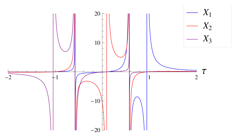
Figure 1: Behaviour of the variables $X_{i}$ given by (83) in General Relativity. Each variable $X_{i}$ has a pole at respective $\tau=\tau_{i}$. These are just special points of the solution, with all connection and metric components remaining finite. Furthermore, all variables $X_{i}$ have common poles at $\tau=\pm\tau_{c}$. These are the singular points for both the connection and the metric. The region ‘between’ two Kasner singularities describes a solution with negative $\Lambda$, while the two outer regions describe solutions with $\Lambda>0$.

We summarise the facts established above. As $\tau\to\infty$, we approach the De Sitter solution $X_{i}=1/{3\tau}$. As time decreases, at $\tau=\tau_{1}$ we encounter a special point where $X_{1}$ has a simple pole, while $X_{2}$ and $X_{3}$ vanish. Below this point, all $X_{i}$ change sign, as does $f(X)$. The component of the connection ${h}_{1}$ vanishes at this point, while the components ${h}_{2}$ and ${h}_{3}$ remain finite. All components of the canonical metric (67) remain finite at this point.

As $\tau\to\tau_{c}$, we approach the Kasner singularity, with the functions $X_{i}$ all negative near the singularity, and all having a simple pole there. The function $N^{2}$ also has a simple pole at this point. The scale factors $a_{i}^{2}$ exhibit the familiar Kasner behaviour (92).

We also note that the region $\tau>\tau_{1}$ is where the solution is guided by the cosmological constant. Near the Kasner singularity, as $\tau\to\tau_{c}$, the Weyl curvature becomes so strong that the cosmological constant does not play any role and can be neglected.

Since the gauge field diverges at the singularity, the domain $-\tau_{c}<\tau<\tau_{c}$ in (83) can only be treated as another singular solution. Let us first consider the region $\tau_{2}<\tau<\tau_{c}$. In order that the metric with components (87) be of the usual signature there, we need to change the sign of the cosmological constant $\Lambda_{0}$. Thus, the solution in this time interval is described by GR with negative cosmological constant. The behaviour near $\tau_{c}$ is again Kasner. The point $\tau_{2}$ again is a special point of the solution, in which $X_{2}$ has a simple pole, while $X_{1}$ and $X_{3}$ have simple zeros. Thus, ${h}_{2}$ passes through zero at this point, with ${h}_{1}$ and ${h}_{3}$ remaining finite and nonzero. The metric components are all finite and non-zero. As $\tau\to-\tau_{c}$, we encounter another Kasner singularity. Thus, the $\Lambda_{0}<0$ part of the solution interpolates between two Kasner singularities. There is no asymptotic anti-De Sitter regime in this case.

For $\tau<-\tau_{c}$, we have another copy of asymptotically De Sitter solution. We note that all $X_{i}$ are positive near the singularity in this case, as is $f(X)$. There is a Kasner singularity as $\tau\to-\tau_{c}$, and a special point at $\tau=\tau_{3}$ with ${h}_{3}$ vanishing and all $X_{i}$ and $f(X)$ changing sign. As $\tau\to-\infty$, we approach another De Sitter region. Since the time change $\tau\to-\tau$ makes the region $\tau<-\tau_{c}$ mathematically equivalent to the asymptotically De Sitter region $\tau>\tau_{c}$ discussed above, it is clear that the Kasner exponents near the singularity in the region $\tau<-\tau_{c}$ are obtained from (93) by the replacement $\tau_{i}\to-\tau_{i}$.

6 One-parameter family of modifications

6.1 Modified $\Lambda_{0}>0$ case

Consider the one-parameter family (18) with $\Lambda_{0}>0$ and small modification $\alpha\Lambda_{0}\ll 1$. In this case, one expects that modification only becomes significant in the region where the Weyl curvature is large, i.e., near the singularity. This is correct, and, as we will see below, the singularity at $\tau=\pm\tau_{c}$ gets resolved in the modified theory, leading to solutions in which the fundamental connection field is regular all through the space-time.

To find solution for $X$, we need to solve equation (82) for $\Psi(\tau)$ and substitute the result into (81). Since, by virtue of (82), $\Psi(\tau)$ is determined by $\Lambda(\tau)$, it will be sufficient to find $\Lambda(\tau)$. To find $X$ from (81) in theory (18), we calculate

$${\rm Id}-\frac{\partial\Lambda}{\partial\Psi}={\rm Id}+\alpha\Psi={\rm Id}+\alpha\Lambda\left(\frac{T^{-1}}{s_{1}}-\frac{1}{3}{\rm Id}\right)\,,$$ (96)

$${\rm Tr\,}\left[T^{-1}\left({\rm Id}-\frac{\partial\Lambda(\Psi)}{\partial\Psi}\right)\right]=s_{1}\left[1+\alpha\Lambda\left(\frac{s_{2}}{s_{1}^{2}}-\frac{1}{3}\right)\right]\,,$$ (97)

where, in addition to (84), we have introduced the function

$$s_{2}={\rm Tr\,}(T^{-2})=\sum_{i}\frac{1}{(\tau-\tau_{i})^{2}}=\frac{3\tau^{4}+6\tau_{1}\tau_{2}\tau_{3}\tau+1}{\prod_{i}(\tau-\tau_{i})^{2}}\,.$$ (98)

Eventually, we have

$$X=\frac{(1-\frac{1}{3}\alpha\Lambda)s_{1}T^{-2}+\alpha\Lambda T^{-3}}{s_{1}^{2}\left(1+\alpha x\Lambda\right)}\,,$$ (99)

where

$$x(\tau)\equiv\left(\frac{s_{2}}{s_{1}^{2}}-\frac{1}{3}\right)=2\frac{3\tau^{2}+9\tau_{1}\tau_{2}\tau_{3}\tau+1}{3\left(3\tau^{2}-1\right)^{2}}\,.$$ (100)

It remains to find $\Lambda(\tau)$. Using (82), we have

$$\Psi^{2}=\Lambda^{2}\left(\frac{T^{-2}}{s_{1}^{2}}-\frac{2T^{-1}}{3s_{1}}+\frac{1}{9}{\rm Id}\right)\,,\qquad{\rm Tr\,}(\Psi^{2})=\Lambda^{2}\left(\frac{s_{2}}{s_{1}^{2}}-\frac{1}{3}\right)\,,$$ (101)

and equation (18) then produces the quadratic equation for $\Lambda(\tau)$:

$$-\frac{\alpha}{2}x(\tau)\Lambda^{2}=\Lambda-\Lambda_{0}\,.$$ (102)

Consider first the region $|\tau|>\tau_{c}$. (The region $|\tau|<\tau_{c}$ is analysed in Section 6.4.) Note that the function $x(\tau)$, defined in (100), is nonnegative and approaches infinity as $|\tau|\to\tau_{c}$. Therefore, in order that the quadratic equation (102) always have a real solution for $\Lambda$, it is necessary to demand that $\alpha>0$. As $|\tau|\to\infty$, the function $x(\tau)$ tends to zero. In order that the solution for $\Lambda$ tend to the general-relativistic value $\Lambda_{0}$ in this limit, one should take the positive root of the quadratic equation (102):

$$\Lambda=\Lambda_{+}=\frac{1}{\alpha x}\left(\sqrt{1+2\alpha x\Lambda_{0}}-1\right)\,.$$ (103)

Since $x$ and $\Lambda$ are both non-negative in the region $|\tau|>\tau_{c}$, the only place where we possibly can encounter singularity in solution (99) is when $s_{1}$ turns to infinity or zero. The first option occurs as $\tau\to\tau_{1}$, at which point the diagonal matrix $T^{-1}$ also becomes singular. The second option occurs as $|\tau|\to\tau_{c}=1/\sqrt{3}$ (this is a singular point in GR). Let us consider these two possibilities separately.

6.2 Behaviour near the pole

As $\tau\to\tau_{1}$, we have $s_{1}\approx 1/(\tau-\tau_{1})\to\infty$, $x\to 2/3$, and, assuming $\alpha\Lambda_{0}\ll 1$ (small modification), $\Lambda\to\Lambda(\tau_{1})\approx\Lambda_{0}$. Solution (99) behaves as in GR and the modification is negligible. This is a special point of the solution, with all $X_{i}$ changing sign there (and one of them, $X_{1}$, having a simple pole). All metric components are finite and non-zero there.

6.3 Behaviour near the would-be singularity

Consider now the critical point. As $\tau\to\tau_{c}$ from above, we have $s_{1}\to 0$ and $x\to\infty$, so that $\Lambda\approx\sqrt{2\Lambda_{0}/\alpha x}\to 0$. We also have $x\approx s_{2}/s_{1}^{2}$ with $s_{2}$ being finite at this point. Therefore, the denominator in (99) behaves as

$$s_{1}^{2}(1+\sqrt{2\alpha\Lambda_{0}x})\approx-s_{1}\sqrt{2\alpha\Lambda_{0}s_{2}}\,,$$ (104)

where we have taken into account that $s_{1}<0$ as we approach $\tau_{c}$ from above. The numerator in (99) behaves as $s_{1}T^{-2}$, with small correction of order $\sqrt{\alpha\Lambda_{0}}$ that can be neglected. Solution (99) then behaves as

$$X_{i}\approx-\frac{1}{\sqrt{2\alpha\Lambda_{0}s_{2}}(\tau-\tau_{i})^{2}}\sim-\frac{1}{\sqrt{\alpha\Lambda_{0}}}\,,$$ (105)

which is large by absolute value (under the assumption $\alpha\Lambda_{0}\ll 1$) but finite.

6.4 Behaviour ‘inside’ the would-be singularity

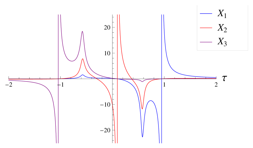
Figure 2: Behaviour of the variables $X_{i}$ given by (99) in the modified theory (18) with $\alpha\Lambda_{0}=5\times 10^{-3}$. As in General Relativity (see Fig. 1), each variable $X_{i}$ has a pole at respective $\tau=\tau_{i}$. However, the common poles at $\tau=\pm\tau_{c}$ disappear, and the variables $X_{i}$ become regular at these points.

In the general-relativistic solution, all $X_{i}$ are negative and blow up near the Kasner singularity $\tau\to\tau_{c}$. In the previous subsection we have seen that modification resolves this singularity, making all $X_{i}$ large negative but finite. Our solution thus smoothly continues to the region $\tau<\tau_{c}$. Since $X_{i}$ are finite and nonzero at this point, $f(X)$ is also continuous. The function $s_{1}$ changes sign from negative to positive as one crosses $\tau_{c}$ from above. In view of the relation $f(X)=s_{1}/\Lambda$ [see (79)], this means that the sign of $\Lambda$ should become negative below the point $\tau_{c}$. To ensure this, we should take the negative root of (102) in the region $|\tau|<\tau_{c}$ :

$$\Lambda=\Lambda_{-}=-\frac{1}{\alpha x}\left(\sqrt{1+2\alpha x\Lambda_{0}}+1\right)\,,$$ (106)

with $x$ defined in (100). Note that this branch of the solution does not have the GR limit as $\alpha\to 0$. Also note that the denominator in (99) is always negative on this branch. One can easily check that solution (99) is continuously differentiable at the point $\tau=\tau_{c}$.

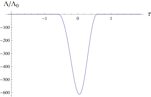
Figure 3: Behaviour of $\Lambda(\tau)/\Lambda_{0}$ in the modified theory (18) with $\alpha\Lambda_{0}=5\times 10^{-3}$.

As time decreases from $\tau_{c}$, the next special point that we encounter is $\tau=\tau_{2}$. Around this point, $s_{1}\approx 1/(\tau-\tau_{2})$, while $x\to 2/3$. Now we have $\Lambda\to\Lambda_{-}(\tau_{2})\approx-3/\alpha$, which is large by absolute value compared to $\Lambda_{0}$. In the neighbourhood of $\tau=\tau_{2}$, solution (99) is then approximated as

$$X=\frac{3T^{-3}-2s_{1}T^{-2}}{s_{1}^{2}}\,.$$ (107)

We observe that $X_{1}$ and $X_{3}$ cross zero at $\tau=\tau_{2}$, while $X_{2}\approx 1/(\tau-\tau_{2})$ has a simple pole, approaching positive infinity as $\tau\to\tau_{2}$ from above. Since all $X_{i}$ were negative at $\tau=\tau_{c}$, this means that $X_{2}$ crosses zero at some $\tau_{+}\in(\tau_{2},\tau_{c})$. It then crosses zero once again at some $\tau_{-}\in(-\tau_{c},\tau_{2})$. This behaviour is demonstrated in Fig. 2. In the interval $(\tau_{-},\tau_{+})$, metric (67) changes signature from $(-,+,+,+)$ to $(-,-,+,-)$, the spatial coordinate $x^{2}$ thus taking the role of time. Thus, although we do not encounter singularity in the fundamental gauge field (all ${h}_{i}$ are everywhere smooth), there is a singularity in metric (67) at the points $\tau=\tau_{\pm}$, where it also changes signature.

It is interesting to plot the behaviour of the ‘cosmological function’ $\Lambda$ for our chosen modification. Since the non-classical branch (106) operates in the time interval $[-\tau_{c},\tau_{c}]$, we have a strongly varying function $\Lambda(\tau)$, greatly deviating from the classical value $\Lambda_{0}$ in this region. This can be clearly seen in the plot of Fig. 3. The limit $\Lambda/\Lambda_{0}\to 1$ as $|\tau|\to\infty$ is invisible in this plot due to resolution.

6.5 Modified $\Lambda_{0}<0$ case

In the case of GR, solution that we obtained in the time interval $(-\tau_{c},\tau_{c})$ was a realisation in the theory with $\Lambda_{0}<0$. In the modified gravity theory described above, we have obtained asymptotically De Sitter solutions with $\Lambda_{0}>0$ in the regions $(\tau_{c},\infty)$ and $(-\infty,-\tau_{c})$ and have shown that they are smoothly connected through a region of strong modified gravity in the interval $(-\tau_{c},\tau_{c})$. At a technical level, the strongly modified solution in the region $(-\tau_{c},\tau_{c})$ resulted from taking the negative root (106) of the quadratic equation (102) for $\Lambda(\tau)$.

In this subsection, we analyse the other possible solution. Specifically, in $(-\tau_{c},\tau_{c})$ we choose the solution of the quadratic equation that has the general-relativistic limit as $\alpha\to 0$. This is the solution that far from the would-be singularity behaves as that in GR with $\Lambda_{0}<0$. After that, we extend the solution beyond the interval $(-\tau_{c},\tau_{c})$ by taking the root (106) of the equation for $\Lambda(\tau)$. In this way, we obtain regions of strongly modified gravity in the intervals $(\tau_{c},\infty)$ and $(-\infty,-\tau_{c})$, connected by an almost GR solution with $\Lambda_{0}<0$ in the interval $(-\tau_{c},\tau_{c})$.

In order that the quadratic equation (102) always have solution for negative $\Lambda_{0}$, we now should require that $\alpha<0$. The expression under the square root in (103) and (106) will then always be positive. As $|\tau|\to\infty$, the function $x(\tau)\sim 2/9\tau^{2}$, so that $\Lambda_{-}(\tau)\sim-2/\alpha x\sim-9\tau^{2}/\alpha$. We thus have a strongly varying ‘cosmological function’ in the regions $(\tau_{c},\infty)$ and $(-\infty,-\tau_{c})$.

It is not hard to repeat the analysis at $\tau=\pm\tau_{c}$ and see that there is no singularity in this solution. However, at some point $\tau_{+}\in(\tau_{c},\tau_{1})$, the variable $X_{1}$ will now turn to zero and change sign. Repeating the analysis of Section 6.4, we conclude that, at this point, we will encounter singularity in metric (67), with a signature change from $(-,+,+,+)$ to $(-,+,-,-)$. A similar event will take place at another point $\tau_{-}\in(\tau_{3},\tau_{c})$, where it will be $X_{3}$ that will pass through zero and change sign. The signature of the metric right below $\tau_{-}$ will then become $(-,-,-,+)$. Furthermore, if $\tau_{2}\neq 0$, then, depending on its sign, the variable $X_{2}$ will also pass through zero and change sign either at some $\tau>\tau_{1}$ (for $\tau_{2}>0$) or at some $\tau<\tau_{3}$ (for $\tau_{2}<0$). The signature of the metric will change accordingly at this point. Asymptotically, by calculating the limits of solution (99) as $|\tau|\to\infty$, we obtain

$$X_{i}\to\tau_{i}+{\cal O}(1/\tau)\,,$$ (108)

The behaviour of $X_{i}$ for $(\tau_{1},\tau_{2},\tau_{3})=(1,0,-1)$ is shown in Fig. 4.

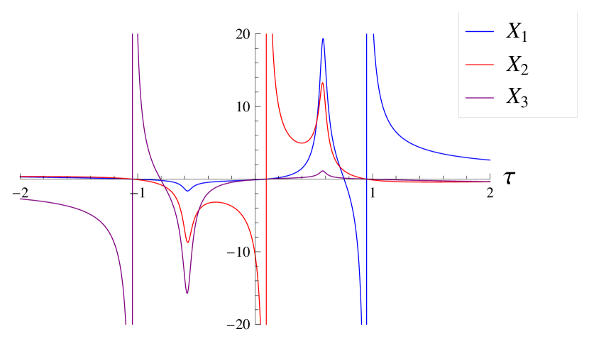
Figure 4: Behaviour of the variables $X_{i}$ in the modified theory (18) with $\Lambda_{0}<0$ and $\alpha\Lambda_{0}=5\times 10^{-3}$.

In this case, the regions $\tau\to\pm\infty$ are singular. Indeed, integrating (54) using (108), and assuming all $\tau_{i}$ to be nonzero, we see that, for large times, ${h}_{i}\propto e^{\tau_{i}\tau}$. Thus, at least one of the connection (and metric) components exponentially blows up, while another exponentially shrinks to zero. This can be regarded as a true singularity of the solution, but ‘delayed’ by the modification to occur at later times. The signature of metric (67) in the asymptotic regions is $(-,-,-,+)$ if $\tau_{2}>0$, and $(-,+,-,-)$ if $\tau_{2}<0$. If $\tau_{2}=0$, then this metric has the first signature in the region $\tau<\tau_{-}$, and the second signature in the region $\tau>\tau_{+}$.

7 Discussion

In this paper, we reviewed the description of the family of chiral modified four-dimensional gravity theories. We used the language of the pure-connection formulation, in which the modification is particularly simple to describe. The idea is simply to consider more general functions of the curvature of the connection than the one that produces the GR dynamics. Such a modification is guaranteed to not lead to higher-order field equations. It may, however, result in the appearance of new propagating degrees of freedom. The chiral family of modified gravity theories considered in this work are known to have degrees of freedom like those present in GR — they continue to propagate just two polarizations of the graviton. Moreover, the argument of [4] based on scattering amplitudes shows that this is the only family of modified vacuum (i.e., not coupled to any matter) gravity theories in four spacetime dimensions that do not increase the number of propagating degrees of freedom.

On the technical side, we have introduced a new parametrisation of this family of theories. Previous studies of these chiral modified theories have used either the first-order BF-type description, as in [5, 6, 7, 8], or the pure-connection description of [21, 22]. The pure-connection formalism is much easier to deal with in practice, as the number of field components that one needs to consider is much smaller. However, it is not free from drawbacks. One of them is the impossibility to deal with the $\Lambda=0$ sector of GR. Another drawback is the presence of the square root in Lagrangian (34), with its several possible branches. Also, the field configurations where the matrix $X^{ij}$ is degenerate (across some surfaces, for example) are problematic in the pure-connection formulation, leading to formal singularities of $0/0$ type in the Euler–Lagrange equations. Finally, it is very difficult to control deviations from GR in the pure-connection formulation. Indeed, it is surprisingly difficult to describe, e.g., modification (18) in the pure-connection language.

All the mentioned drawbacks disappear if one allows oneself to keep, in addition to the connection, a matrix $M^{ij}$ of auxiliary fields. One can then easily treat GR with zero cosmological constant, as we show in the Appendix on the example of the Bianchi I cosmology. There is no more need to take the matrix square root $X^{ij}$ in obtaining the GR solution. Thus, configurations where one of the eigenvalues of the matrix $X^{ij}$ turns to zero are no longer a problem, as we explicitly saw in the analysis of the GR solution in Section 5. It is also easy to describe controlled modifications of GR of the type (18), as we have seen in Section 6. All in all, we feel that ‘mixed’ parametrisation introduced in this paper is superior to the pure-connection one, in the sense of keeping all its advantages (it is still a connection rather than metric formulation), while avoiding its drawbacks. This formulation has already been put to use for other problems, see [9], [10]

The family of modifications of four-dimensional General Relativity that was described in this paper is chiral. As a result, it is, in fact, a modification of complexified GR. It is not difficult to state the reality conditions leading to Riemannian and split signatures in the modified theories. However, no reality condition appropriate for the physical Lorentzian signature is yet known, at least not in full generality. So, as things stand, it is not clear whether the modified gravity theories described here admit physical interpretation.

Nevertheless, there are situations where the chiral character of the theory causes no difficulty. In this paper, we have studied one such situation. In Bianchi I spacetimes, the self-dual part of the Weyl curvature is real (even in Lorentzian signature). As a result, the modifications, described here, that effectively introduce the powers of the self-dual part of the Weyl curvature to the Lagrangian do not make the Lagrangian complex. Because of this, the metric arising in these modified theories can be taken to be real. In this paper, we obtained the behaviour of such real metrics in the Bianchi I setup by solving the evolution equations for the connection components and reading the metric from the connection.

Our main finding is that a natural one-parameter family of modifications (18), with a specific choice of the sign of the parameter $\alpha$ controlling the modification, resolves the Kasner singularity of Bianchi I spacetimes. In the most interesting case of modified gravity with a positive cosmological constant, we obtain a solution connecting two asymptotically De Sitter regions. This solution, depicted in Fig. 2, avoids the two would-be Kasner singularities of GR, and the fundamental connection field remains regular all through the space-time. Between the two would-be singularities, there lies a region of strong modification of gravity. Inside this region, there are two moments of time where the metric becomes singular, while the basic fields of the theory (the connection components), as we have said, remain finite. This behaviour is similar to what was observed in the case of modified black-hole solution in [6]. This type of metric singularity in the absence of any singularity in the basic connection fields appears to be generic to the modified theories under investigation.

The fact that modified gravity theories of this kind avoid so nicely the singularities of GR solutions suggests that they are more than just mathematical curiosities. At the same time, as we already noted, their physical interpretation is not clear at present. In a more general setting, it is no longer possible to require that the metric as defined by the connection via (35) is real Lorentzian, as this is simply incompatible with the dynamics. It is not yet clear how this inherent complexity of the theory should be treated. There might exist some choice of reality conditions that reduces the dynamics to a half-dimensional slice through the phase space with real-valued Hamiltonian and symplectic form on this slice. If this is the case, such a real slice would provide the sought interpretation.

A related problem is that of coupling to matter. The fundamental field of our gravity theories is a connection, to which the matter fields should couple directly. Such coupling in the case of GR can be obtained by the same trick of integrating out the metric. Indeed, in the first-order formalism, all matter Lagrangians are algebraic in the metric (i.e., do not contain derivatives of $g_{\mu\nu}$). Thus, in principle at least, the metric can still be integrated out to produce a connection–plus–matter formulation. In practice, however, this may be difficult. Further, it is not clear how to modify such gravity–plus–matter theories. Alternatively, one can start with a more general family of gauge theories as described in [24]. These describe gravity as well as matter fields. So, some type of matter couplings can be obtained in this way. But the problem of finding the correct reality conditions still remains in any setting — since matter fields couple to a complex-valued connection, some reality conditions are required to make sense of the arising dynamics.

We end this paper by noting that the problem of reality conditions is the most pressing one as far as classical theory is concerned. We hope that the results presented here, even though not immediately concerned with this problem, will serve as a step towards developing a physical interpretation of the modified gravity theories under consideration.

Appendix: Chirality

The aim of this section is to review briefly some basic facts about spinors and self-duality in four space-time dimensions. This will clarify our usage of the term ‘chirality’ in this paper.

In the sense used in this paper, the notion of chirality is related to the fact that the four-dimensional Lorentz group is doubly covered by the Möbius group ${\rm SL}(2,{\mathbb{C}})$. The fundamental irreducible representations of the latter are of two different types: 2-component columns $\lambda$ on which $2\times 2$ matrices $g\in{\rm SL}(2,{\mathbb{C}})$ act as $\lambda\to g\lambda$, and the complex conjugate representation in terms of 2-component columns $\bar{\lambda}$ on which the action is $\bar{\lambda}\to g^{*}\bar{\lambda}$, where $g^{*}$ is the complex conjugate matrix. Members of these two different representation spaces are spinors of two different types that exist in four dimensions. These 2-component spinors are chiral objects: taking the complex conjugate of a spinor of one type, one obtains a spinor of the different type. This operation of complex conjugation is related to the three-dimensional operation of taking the mirror image (see below), which justifies using the terminology ‘chiral’ also in reference to complex conjugation.

As is well-known, a 4-vector can equivalently be thought of as a bi-spinor of a mixed type. Thus, if we refer to the spinor representation of the first type as $S_{+}$ and to that of the second type as $S_{-}$, then the vector representation is isomorphic to $S_{+}\otimes S_{-}$. Real elements of this space are represented by $2\times 2$ Hermitian matrices ${\bf x}={\bf x}^{\dagger}$ on which the Lorentz group acts as ${\bf x}\to g{\bf x}g^{\dagger}$, where $g^{\dagger}=(g^{T})^{*}$ is the Hermitian conjugate of $g$. It is this representation of 4-vectors as Hermitian matrices that provides the local isomorphism ${\rm SO}(1,3)\sim{\rm SL}(2,C)$. Taking the complex conjugate of $S_{+}$, one gets $S_{-}$. Thus, the space $S_{+}\otimes S_{-}$ has a subspace of real, or non-chiral, objects, and these are precisely the (real) 4-vectors.

A related chiral decomposition exists in the space of 2-forms in four dimensions. Indeed, given a metric, we have the operation of taking the Hodge dual of a differential form. This operation maps the space of 2-forms into itself. In the case of Lorentzian signature, repeating this operation twice gives minus the identity operator: $*^{2}=-1$. The eigenspaces of $*$ in the space $\Lambda^{2}_{\mathbb{C}}$ of complexified 2-forms are then referred to as the spaces of self-dual $\Lambda^{+}$ and anti-self-dual $\Lambda^{-}$ 2-forms. Any 2-form can be split into its self-dual and anti-self-dual parts $\Lambda^{2}=\Lambda^{+}\oplus\Lambda^{-}$. Real-valued 2-forms then satisfy the condition that their self-dual and anti-self-dual parts are the complex conjugates of each other. This decomposition of $\Lambda^{2}$ is related to the spinor story we reviewed above because $\Lambda^{+}$ can be shown to be isomorphic to $S_{+}^{2}$, the second symmetric power of the fundamental representation of the first type. This is realised as the space of rank 2 spinors that are symmetric in their 2 spinor indices. Similarly $\Lambda^{-}\sim S_{-}^{2}$. The operation of complex conjugation takes $S_{+}$ to $S_{-}$, and so there are real elements in $S_{+}^{2}\oplus S_{-}^{2}$. These are real-valued 2-forms. It can also be checked that the operation of taking the mirror image, e.g., reflecting one of the spatial coordinates, interchanges the spaces $\Lambda^{+}$ and $\Lambda^{-}$. In this sense, the mirror reflection is the same as complex conjugation.

Appendix: The sector of interest

In this Appendix, we derive the diagonal ansatz used in the main text from more general considerations.

We are interested in a general spatially homogeneous but anisotropic sector of the theory. This is described by an ${\rm SO}(3)$ connection with components $A^{i}$ that are functions of the time coordinate $\tau$ only. A general such connection is of the form

$$A^{i}=a^{ij}dx^{j}+b^{i}d\tau\,,$$ (109)

where $a^{ij}$ and $b^{i}$ are (complex-valued in general) functions of the time coordinate $\tau$. Performing a time-dependent ${\rm SO}(3,{\mathbb{C}})$ transformation, one can always make the matrix $a^{ij}$ symmetric. After that, using $\tau$-dependent spatial translations, one can always set the $b$-components to zero.

Thus, gauge-fixing the spatial diffeomorphisms and the gauge rotations, we are led to consider the following sector of the theory:

$$A^{i}=a^{ij}dx^{j}\,,$$ (110)

where $a^{ij}$ is a symmetric matrix of arbitrary (complex-valued) functions of the time coordinate only. In more mathematical language, the time evolution of our system is a trajectory on the homogeneous group manifold

$${\rm GL}(3,{\mathbb{C}})/{\rm SO}(3,{\mathbb{C}})\,,$$ (111)

parametrised by symmetric complex-valued $3\times 3$ matrices. We have not yet imposed any reality conditions, this will be done below.

Field equations

The field equations in the pure-connection theory are

$$d_{A}\left(\frac{\partial f}{\partial X^{ij}}\right)\wedge F^{j}=0\,,$$ (112)

where the matrix $X^{ij}$ is defined as in (25) and, in view of the homogeneity of the function $f(\cdot)$, it does not matter precisely which volume form is chosen in (25).

For the connection (110) we have:

$$F^{i}=\dot{a}^{ij}d\tau\wedge dx^{j}+\frac{1}{2}(a^{-1})^{ij}{\rm det\,}a\,\epsilon^{jkl}dx^{k}\wedge dx^{l}\,,$$ (113)

where we have assumed the matrix $a^{ij}$ to be invertible, and the dot denotes the derivative with respect to $\tau$. Correspondingly, the matrix of the wedge products of the curvature is given by:

$$F^{i}\wedge F^{j}=2\dot{a}^{(i|k|}(a^{-1})^{j)k}{\rm det\,}a\,d\tau\wedge dx^{1}\wedge dx^{2}\wedge dx^{3}\,,$$ (114)

so that

$$X^{ij}\propto\dot{a}^{(i|k|}(a^{-1})^{j)k}\,,$$ (115)

where the proportionality means equality modulo an arbitrary function of time.

Now we can write the field equations. It is not hard to check that the $dx^{i}\wedge dx^{j}\wedge dx^{k}$ component of equations (112) holds automatically, in view of the symmetry of the matrix of first derivatives of the function $f(X)$. Thus, we only need to consider the $\epsilon^{ijk}d\tau\wedge dx^{j}\wedge dx^{k}$ part. This part reads:

$$\left(\frac{\partial f}{\partial X^{ij}}\right)^{\cdot}(a^{-1})^{jk}{\rm det\,}a-\epsilon^{ipl}\epsilon^{mnk}a^{pm}\dot{a}^{jn}\frac{\partial f}{\partial X^{lj}}-\epsilon^{jpl}\epsilon^{mnk}a^{pm}\dot{a}^{jn}\frac{\partial f}{\partial X^{li}}=0\,.$$ (116)

It is convenient to multiply this equation by $a^{qk}$ and divide by ${\rm det\,}a$. After some simple algebra, we get

$$\left(\frac{\partial f}{\partial X^{ij}}\right)^{\cdot}+\frac{\partial f}{\partial X^{ij}}\,{\rm Tr\,}X+\frac{\partial f}{\partial X^{jk}}(X+Y)^{ki}-\frac{\partial f}{\partial X^{ik}}(X+Y)^{jk}=\delta^{ij}\,{\rm Tr\,}\left(\frac{\partial f}{\partial X}X\right)\,.$$ (117)

Here, we have introduced the notation

$$\dot{a}^{ik}(a^{-1})^{jk}=X^{ij}+Y^{ij}\,,$$ (118)

where $X$ and $Y$ are the symmetric and antisymmetric parts, respectively. Now, in view of the gauge invariance of the function $f(X)$, we have:

$$\frac{\partial f}{\partial X^{jk}}X^{ki}-\frac{\partial f}{\partial X^{ik}}X^{kj}=0\,,$$ (119)

and only the $Y$-part survives in the third and fourth terms in (117). We can also use the homogeneity of $f(X)$ that implies

$${\rm Tr\,}\left(\frac{\partial f}{\partial X}X\right)=f\,.$$ (120)

Eventually, we get the differential equation for $X^{ij}$:

$$\left(\frac{\partial f}{\partial X^{ij}}\right)^{\cdot}+\frac{\partial f}{\partial X^{ij}}{\rm Tr\,}X+\frac{\partial f}{\partial X^{ik}}Y^{kj}+\frac{\partial f}{\partial X^{jk}}Y^{ki}=\delta^{ij}f(X)\,.$$ (121)

Note that both the left-hand and right-hand side are explicitly symmetric in $ij$, as they should be.

Reality conditions

Let us now impose the reality conditions (36). For the sector of interest, they read

$$\dot{a}^{ik}(\bar{a}^{-1})^{jk}{\rm det\,}\bar{a}+(\dot{\bar{a}})^{jk}(a^{-1})^{ik}{\rm det\,}a=0\,.$$ (122)

We will not attempt at finding the most general solution of this equation, considering instead a particular ansatz sufficient for our purposes. Thus, we require that $a^{ij}$ are all purely imaginary:

$$a^{ij}={\rm i}{h}^{ij}\,,\qquad{h}^{ij}\in{\mathbb{R}}\,.$$ (123)

Condition (122) then boils down to

$$(\dot{{h}}{h}^{-1})^{[ij]}=0\,.$$ (124)

This, in particular, implies that $Y^{ij}=0$ in (121).

Condition (124) can be stated as requiring that the matrices $\dot{{h}}$ and ${h}$ commute at all times. Let us consider some initial moment of time. Then we can simultaneously diagonalise both of these symmetric matrices by an orthogonal transformation. Then the evolution equations (121) can be seen to imply that if $\dot{{h}}$ and ${h}$ are diagonal at the initial moment of time, they will stay diagonal. So, without loss of generality, we can assume ${h}^{ij}$ to be diagonal at all times:

$${h}^{ij}={\rm diag}({h}_{1},{h}_{2},{h}_{3})\,.$$ (125)

The evolution equations then take the following simple form:

$$\left(\frac{\partial f}{\partial X^{ij}}\right)^{\cdot}+\frac{\partial f}{\partial X^{ij}}{\rm Tr\,}X=\delta^{ij}f(X)\,,$$ (126)

$$X^{ij}={\rm diag\,}\left(X_{1}\,,X_{2}\,,X_{3}\right)\,,\qquad X_{i}=\frac{\dot{h}_{i}}{{h}_{i}}\,.$$ (127)

It can, moreover, be assumed that all matrices appearing here are diagonal.

System (126), (127) can be viewed as a system of second-order differential equations for the functions ${h}_{1}$, ${h}_{2}$, and ${h}_{3}$. However, it is more convenient to view (126) as a system of first-order differential equations for the components of the (diagonal) symmetric matrix $X^{ij}$. Once these are found, the components of the connection can be found by integrating equation (127). The function $f(X)$ should be considered as given. In the main text, we study equations (126) using the parametrisation of the function $f(X)$ in terms of $M$, as described in Section 2.

Appendix: GR solution in the physical time

In this section, we find the GR solution of the Bianchi I model working in the physical time coordinate, see below. We give it here for completeness, as well as to stress the point that the time variable used in the main text simplifies it considerably.

For the function $f(X)$ given by (34), which corresponds to general relativity, equation (56) reduces to

$$\left(\frac{\sum_{j}y_{j}}{y_{i}}\right)^{\cdot}=\left(\sum_{j}y_{j}\right)^{2}-\frac{\sum_{j}y_{j}}{y_{i}}\sum_{j}y_{j}^{2}\,,$$ (128)

where $y_{j}=\sqrt{X_{j}}$ is understood as some branch of the square root.

The physical time

It is clear from (67) that the choice of physical time corresponds to the following condition

$${\rm Tr\,}\sqrt{X}{\rm det\,}\sqrt{X}=\Lambda\,,$$ (129)

where $\Lambda$ is, in fact, the cosmological constant, which, for definiteness, we assume to be positive. We shall denote the physical time by $t$.

Solution in the physical time

Let us choose to parametrise $X_{i}$ as follows:

$$X_{i}=\frac{\epsilon_{ijk}H_{j}H_{k}}{2H_{i}}\,.$$ (130)

Condition (129) then takes the form familiar from the Bianchi I cosmology, in which $H_{i}$ play the role of the Hubble parameters:

$$H_{2}H_{3}+H_{3}H_{1}+H_{1}H_{2}=\Lambda\,.$$ (131)

We then have

$$\sum_{j}y_{j}=\left(H_{1}H_{2}H_{3}\right)^{-1/2}\,,\qquad\frac{\sum_{j}y_{j}}{y_{i}}=\frac{2}{\epsilon_{ijk}H_{j}H_{k}}\,.$$ (132)

Substituting these expressions into (128) and using constraint (131), we obtain the usual evolution equations for the Bianchi I cosmology:

$$\dot{H}_{i}+H_{i}^{2}=\frac{1}{2}\epsilon_{ijk}H_{j}H_{k}\,.$$ (133)

Solution of these equations can be parametrised by angle $\theta$ and presented in the form

$$\begin{array}[]{l}H_{1}=\displaystyle\frac{1}{3\sqrt{\Lambda}}\left[\coth\sqrt{\Lambda}t+\frac{2\sin\theta}{\sinh\sqrt{\Lambda}t}\right]\,,\vskip 12.0pt plus 4.0pt minus 4.0pt\\ H_{2}=\displaystyle\frac{1}{3\sqrt{\Lambda}}\left[\coth\sqrt{\Lambda}t+\frac{2\sin\left(\theta+\frac{2\pi}{3}\right)}{\sinh\sqrt{\Lambda}t}\right]\,,\vskip 12.0pt plus 4.0pt minus 4.0pt\\ H_{3}=\displaystyle\frac{1}{3\sqrt{\Lambda}}\left[\coth\sqrt{\Lambda}t+\frac{2\sin\left(\theta-\frac{2\pi}{3}\right)}{\sinh\sqrt{\Lambda}t}\right]\,.\end{array}$$ (134)

For $\Lambda>0$, it describes the Kasner regime as $t\to 0$ and proceeds to the De Sitter space asymptotically as $t\to\infty$. For $\Lambda<0$, the solution is obtained by analytic continuation, and describes evolution between two Kasner-like singularities.

The above solution for $H$’s gives us the functions $X_{1}$, $X_{2}$, and $X_{3}$. We then can integrate (54) and get the components of the connection. An equivalent, but simpler procedure is to look for ${h}$’s in the parametrisation

$${h}_{i}=H_{i}a_{i}\,,$$ (135)

where $a_{i}$ are some yet unknown functions. Then, if we write

$$\frac{H_{2}H_{3}}{H_{1}}=\frac{(H_{1}a_{1}){}^{\cdot}}{H_{1}a_{1}}=\frac{(H_{2}H_{3}-H_{1}^{2})a_{1}+H_{1}\dot{a_{1}}}{H_{1}a_{1}}\,,$$ (136)

where we have used one of equations (133), we see that

$$\frac{\dot{a_{i}}}{a_{i}}=H_{i}\,,$$ (137)

which allows one to solve for $a_{i}$ and then get the functions ${h}_{i}$ from (135). From (59), we also note that the functions $a_{i}$ are precisely the scale factors of the metric, i.e.,

$$ds^{2}=-dt^{2}+\sum_{i}a_{i}^{2}(dx^{i})^{2}.$$ (138)

In the next section, we show how to obtain the GR solution in a simpler way by choosing a different time coordinate.

Appendix: GR with zero cosmological constant

In this Appendix, we find the solution of GR with zero cosmological constant using our mixed parametrisation. The purpose of this exercise is to see that the mixed parametrisation can be readily used to solve the equations of GR with $\Lambda=0$, where no pure-connection formulation is available.

For the same Bianchi I ansatz, the evolution equations take the following form. First, there is equation (58), which in this case takes the form

$$\left(\Psi_{i}^{-1}{h}\right)^{\cdot}={\rm Tr\,}\left(\Psi^{-1}X\right){h}=0\,,$$ (139)

where the zero right-hand side follows from equation (43). We then get

$$\Psi_{i}=\sigma_{i}{h}\,,$$ (140)

where $\sigma_{i}$ are nonzero integration constants.

Equation (43) and the tracelessness of $\Psi$ then imply, respectively,

$$X_{i}=\zeta(\tau)\sigma_{i}^{2}\,,\qquad\sum_{i}\sigma_{i}=0\,,$$ (141)

where $\zeta(\tau)$ in the first equation is some function of time. The second equation entails a useful relation

$$\sum_{i}\sigma_{i}^{4}=\sum_{i\neq j}\sigma_{i}^{2}\sigma_{j}^{2}\,.$$ (142)

We look for solution of the theory in the form of power law:

$${h}_{i}(\tau)=C_{i}\tau^{m_{i}}\,,$$ (143)

with some exponents $m_{i}$. With this ansatz for the solution, we have

$$X_{i}=\frac{\dot{{h}}_{i}}{{h}_{i}}=\frac{m_{i}}{\tau}\,.$$ (144)

Equations (141) give $\zeta(\tau)=C/\tau$, and imply the following relations between $m_{i}$ and $\sigma_{i}$ :

$$m_{i}=C\sigma_{i}^{2}\,.$$ (145)

Equation (142) then gives

$$\sum_{i}m_{i}^{2}=\sum_{i\neq j}m_{i}m_{j}\,.$$ (146)

We now need to specify the time coordinate which, up to now, was quite arbitrary. Let us choose $\tau$ to be the physical time coordinate $t$, in which $N^{2}(t)\equiv 1$. Declaring the curvature two-forms to be self-dual, we get relations (62). With the above choice for the lapse function, this gives

$$a_{1}^{2}=\frac{C_{1}^{2}}{m_{2}m_{3}}t^{2(m_{1}+1)}\,,\quad{\rm etc}\,.$$ (147)

On the other hand, according to (15), the metric volume form (63) should be a multiple of

$${\rm Tr}\left(B\wedge B\right)={\rm Tr}\left(\Psi^{-1}F\wedge\Psi^{-1}F\right)\propto{\rm Tr\,}(\Psi^{-2}X){h}{\cal V}_{c}$$ (148)

[see (53)]. This gives

$$\prod_{i}a_{i}\equiv\left|\frac{{h}}{\prod_{i}X_{i}}\right|\propto\left({h}t\right)^{-1}\,,$$ (149)

which, in turn, implies ${h}(t)\propto t^{-2}$, and

$$\sum_{i}m_{i}=-2\,.$$ (150)

Comparing (147) to the Kasner metric (95) we see that we must identify

$$m_{i}=p_{i}-1\,.$$ (151)

Then (150) takes the familiar form

$$\sum_{i}p_{i}=1\,,$$ (152)

and (146) implies

$$\sum_{i}p_{i}^{2}=1\,.$$ (153)

We thus recover the Kasner solution.

References

- [1] M. F. Atiyah, N. J. Hitchin and I. M. Singer, “Self-Duality in Four-Dimensional Riemannian Geometry,” Proc. Roy. Soc. Lond. A 362, 425 (1978).
- [2] A. A. Starobinsky, “A New Type of Isotropic Cosmological Models Without Singularity,” Phys. Lett. B 91, 99 (1980).
- [3] P. A. R. Ade et al. [Planck Collaboration], “Planck 2015 results. XX. Constraints on inflation,” arXiv:1502.02114 [astro-ph.CO].
- [4] K. Krasnov, “GR uniqueness and deformations,” JHEP 1510, 037 (2015) doi:10.1007/JHEP10(2015)037 [arXiv:1410.8006 [hep-th]].
- [5] K. Krasnov, “Non-Metric Gravity. I. Field Equations,” Class. Quant. Grav. 25, 025001 (2008) [gr-qc/0703002].
- [6] K. Krasnov and Y. Shtanov, “Non-Metric Gravity. II. Spherically Symmetric Solution, Missing Mass and Redshifts of Quasars,” Class. Quant. Grav. 25, 025002 (2008) [arXiv:0705.2047 [gr-qc]].
- [7] K. Krasnov and Y. Shtanov, “Halos of Modified Gravity,” Int. J. Mod. Phys. D 17, 2555 (2009) [arXiv:0805.2668 [gr-qc]].
- [8] K. Krasnov and Y. Shtanov, “Cosmological perturbations in a family of deformations of general relativity,” JCAP 1006, 006 (2010) [arXiv:1002.1210 [gr-qc]].
- [9] J. Fine, Y. Herfray, K. Krasnov and C. Scarinci, “Asymptotically hyperbolic connections,” arXiv:1512.07109 [gr-qc].
- [10] K. Krasnov, “Deformations of GR and BH thermodynamics,” Class. Quant. Grav. 33, no. 15, 155012 (2016) [arXiv:1512.07110 [gr-qc]].
- [11] P. Peldan, “Connection formulation of (2+1)-dimensional Einstein gravity and topologically massive gravity,” Class. Quant. Grav. 9, 2079 (1992).
- [12] P. Peldan, “Actions for gravity, with generalizations: A Review,” Class. Quant. Grav. 11, 1087 (1994) [gr-qc/9305011].
- [13] T. Basile, X. Bekaert and N. Boulanger, “Note about a pure spin-connection formulation of general relativity and spin-2 duality in (A)dS,” Phys. Rev. D 93, no. 12, 124047 (2016) [arXiv:1512.09060 [hep-th]].
- [14] R. De Pietri and L. Freidel, “so(4) Plebanski action and relativistic spin foam model,” Class. Quant. Grav. 16, 2187 (1999) [gr-qc/9804071].
- [15] J. F. Plebanski, “On the separation of Einsteinian substructures,” J. Math. Phys. 18, 2511 (1977).
- [16] R. Capovilla, T. Jacobson, J. Dell and L. J. Mason, “Selfdual two forms and gravity,” Class. Quant. Grav. 8, 41 (1991).
- [17] K. Krasnov, “Plebanski Formulation of General Relativity: A Practical Introduction,” Gen. Rel. Grav. 43, 1 (2011) [arXiv:0904.0423 [gr-qc]].
- [18] H. Urbantke, “On Integrability Properties Of Su(2) Yang–Mills Fields. I. Infinitesimal Part,” UWTHPH-1984-02.
- [19] K. Krasnov, “Renormalizable Non-Metric Quantum Gravity?,” hep-th/0611182.
- [20] K. Krasnov, “On deformations of Ashtekar’s constraint algebra,” Phys. Rev. Lett. 100, 081102 (2008) [arXiv:0711.0090 [gr-qc]].
- [21] K. Krasnov, “Gravity as a diffeomorphism invariant gauge theory,” Phys. Rev. D84, 024034 (2011) [arXiv:1101.4788 [hep-th]].
- [22] K. Krasnov, “Pure Connection Action Principle for General Relativity,” Phys. Rev. Lett. 106, 251103 (2011) [arXiv:1103.4498 [gr-qc]].
- [23] D. Beke, “Plebanski’s Formalism and Modified Gravity,” PhD Thesis, Universiteit Gent (2012).
- [24] K. Krasnov, “Spontaneous Symmetry Breaking and Gravity,” Phys. Rev. D 85, 125023 (2012) [arXiv:1112.5097 [hep-th]].