Hadronic light-by-light contribution to $a_{\mu}$: extended Nambu-Jona-Lasinio, chiral quark models and chiral Lagrangians

Abstract

This talk discusses our old work on the hadronic light-by-light contribution to the muon anomalous magnetic moment and some more recent contributions. I discuss the various contributions starting with pseudo-scalar meson exchange, the quark- and pion-loop, as well as scalar and $a_{1}$-exchange. For the $\pi^{0}$-exchange I point out a possible large enhancement when only connected contributions are included. For the quark-loop I include some comments about the more recent estimates of this contribution. The pion-loop is discussed in more detail, in particular I discuss our unpublished work on including effects from $a_{1}$ and the polarizability.

LU TP 15-46
October 2015

 
^∗ Invited talk FCCP2015 - Workshop on “Flavour changing and conserving processes,” 10-12 September 2015, Anacapri, Capri Island, Italy.

1 Introduction

There were many talk on the muon anomalous magnetic moment and hadronic contributions to it at this conference. This manuscript should be read together with those. A general introduction to the theory of the hadronic contributions to the muon anomaly $a_{\mu}=(g_{\mu}-2)/2$ was given in the talks by Melnikov Melnikov and Knecht Knecht . The hadronic light-by-light-contribution (HLbL) shown in Fig. 1 was discussed in the talks by Procura Procura ,

Figure 1: HLbL contribution to the muon $g-2$. The crossed blob indicates the strong interaction part.

Cappiello Cappiello , Greynat Greynat , Nyffeler Nyffeler , Lehner Lehner and Vanderhaeghen Vanderhaeghen . There were also several talks on the underlying form-factors, both theoretically and experimentally.

The main reason is the measurement of the muon anomalous magnetic moment of Bennett:2006fi and the discrepancy with the satandard model prediction. Reviews of the theory can be found in Bijnens:2007pz ; Prades:2009tw ; Jegerlehner:2009ry but more references and reviews can be found in the remainder of this talk and the talks mentioned above. The main conclusion was that the present best estimate of the HLbL is $(11\pm 4)\times 10^{-10}$ Bijnens:2007pz ; Jegerlehner:2009ry or $(10.5\pm 2.6)\times 10^{-10}$ Prades:2009tw . The main difference is an estimate of the errors which is always somewhat subjective.

In this talk I will concentrate on the work done a long time ago Bijnens:1995cc ; Bijnens:1995xf ; Bijnens:2001cq as well as some newer work on the pion loop. I will also discuss more recent contributions about the pseudo-scalar exchange and quark-loop. I do not present a new final overall number but will argue that a good estimate for the pion-loop contribution is $-(2.0\pm 0.5)\times 10^{-10}$.

A short overview of general properties of the underlying four-point functions is Sect. 2 followed by a reminder of the ENJL model used for a large part of Bijnens:1995cc ; Bijnens:1995xf ; Bijnens:2001cq in Sect. 3. Sect. 4 discusses the numerically largest contribution, pseudo-scalar meson exchange. The contribution with rather large theoretical errors, the quark-loop, is discussed in Sect. 5. Other leading large $N_{c}$ exchanges are scalar, Sect. 6, and $a_{1}$-exchange, Sect. 7. I spent a large amount of space on the $\pi$-loop contribution since that is where I have some new results to present. Details are in Sect. 8. I present some conclusions and some possible future directions in the last section.

2 General properties

The problem is that the integration over photon momenta $p_{1},p_{2}$ in the diagram in Fig. 1 contains both high and low moimenta and mixed cases. Double counting is thus a serious issue when using both quark and hadron contributions. Ref. deRafael:1993za suggested using chiral $p$ and large $N_{c}$ counting to distinguish different contributions. This does not fully solve the double counting issue but it is a good start. This suggestion was followed by two groups doing a more or less full evaluation of the HLbL, the one I was involved in Bijnens:1995cc ; Bijnens:1995xf ; Bijnens:2001cq (BPP) and Kinsohita and collaborators Hayakawa:1995ps ; Hayakawa:1996ki ; Hayakawa:1997rq (HKS). In fact, these are still the only full calculations that exist.

The underlying object is the four-point function $\Pi^{\rho\nu\alpha\beta}(p_{1},p_{2},p_{3})$ of four electromagnetic vector currents. In fact what we really need is a derivative w.r.t. $p_{3}$ at $p_{3}=0$,

$$\left.{\delta\Pi^{\rho\nu\alpha\beta}(p_{1},p_{2},p_{3})\over\delta p_{3\lambda}}\right|_{p_{3}=0}\,.$$ (1)

$\Pi^{\rho\nu\alpha\beta}(p_{1},p_{2},p_{3})$ has in general 138 Lorentz structures which reduces to 43 gauge-invariant structures. Note that in four dimensions there really are 2 less, 136 and 41 Eichmann:2014ooa . Of the 138 more general structures 28 JBJR actually contribute (improving the 32 estimate of Bijnens:1995xf ). Each of these functions depends on $p_{1}^{2},p_{2}^{2},q^{2}$ and before the derivative also on $p_{3}^{2},p_{1}.p_{3},p_{2}.p_{3}$. This should be compared with the lowest order hadronic vacuum polarization where there is one function of one variable. There are two groups using dispersive methods to to establish a link to experiment as close as possible. These were covered in the talks by Procura Procura and Vanderhaeghen Vanderhaeghen .

After setting $p_{3}\to 0$ the loop integrals over the photon momenta is 8 dimensional. Three of these integrations are trivial and using Gegenbauer polynomial methods two more can be done Jegerlehner:2009ry ; JBJR ; Knecht:2001qf . So, after having a model or a computation of $\Pi^{\rho\nu\alpha\beta}(p_{1},p_{2},p_{3})$ there is a triple integral over $p_{1}^{2},p_{2}^{2},q^{2}$ left. The components and their derivatives then become mulitplied with functions of $p_{1}^{2},p_{2}^{2},q^{2}$ examples of which are in Jegerlehner:2009ry ; Knecht:2001qf and the full results can be found in JBJR . In the work I have been involved in we have done the relevant integrations in Euclidean space, i.e. with $P_{1}^{2},P_{2}^{2},Q^{2}=-p_{1}^{2},-p_{2}^{2},-q^{2}$ always positive.

How models actually contribute to the muon anomaly $a_{\mu}$ can be studied by rewriting the integral over $P_{1}^{,}P_{2}^{2},Q^{2}$ in the form Bijnens:2007pz

$$a_{\mu}=\int dl_{P_{1}}dl_{P_{2}}\,{a_{\mu}^{\mathrm{LL}}}=\int dl_{P_{1}}dl_{P_{2}}dl_{Q}\,{a_{\mu}^{\mathrm{LLQ}}}$$ (2)

with $l_{P}=(1/2)\ln\left(P^{2}/\mathrm{G}eV^{2}\right)$. The reason for choosing the logarithm is that this way it is easiest to see which momentum region contributes. Alternatively one can integrate each momentum up to a cut-off $\Lambda$.

One should remember that the different contributions are usually defined within a given model or approach. What is included under the same name can therefore differ and one should be careful when drawing conclusions from comparing calculations.

3 The ENJL model

The main model underlying the work of Bijnens:1995cc ; Bijnens:1995xf ; Bijnens:2001cq is the extended Nambu-Jona-Lasinio (ENJL) as introduced in Bijnens:1992uz ; Bijnens:1995ww . The Lagrangian is given by

$${\cal L}_{\rm ENJL}= \overline{q}^{\alpha}\left\{i\gamma^{\mu}\left(\partial_{\mu}-iv_{\mu}-ia_{\mu}\gamma_{5}\right)-\left({\cal M}+s-ip\gamma_{5}\right)\right\}q^{\alpha}$$

$$+2\,g_{S}\,\left(\overline{q}^{\alpha}_{R}q^{\beta}_{L}\right)\left(\overline{q}^{\beta}_{L}q^{\alpha}_{R}\right)$$

$$-g_{V}\,\left[\left(\overline{q}^{\alpha}_{L}\gamma^{\mu}q^{\beta}_{L}\right)\left(\overline{q}^{\beta}_{L}\gamma_{\mu}q^{\alpha}_{L}\right)+\left(\overline{q}^{\alpha}_{R}\gamma^{\mu}q^{\beta}_{R}\right)\left(\overline{q}^{\beta}_{R}\gamma_{\mu}q^{\alpha}_{R}\right)\right]$$

with $\overline{q}\equiv\left(\overline{u},\overline{d},\overline{s}\right)$. $v_{\mu}$, $a_{\mu}$, $s$, $p$ are the usual external vector, axial-vector, scalar and pseudoscalar matrix sources as used in Chiral Perturbation Theory. ${\cal M}$ is the quark-mass matrix. This model has no confinement but spontaneous symmetry breaking and has good pion, vector meson and OK axial vector-meson phenomenology. The usual NJL model does not have the $g_{V}$ term and does not include (axial) vector mesons. The states are dynamically realized via bubble resummation. The simplicity of the model and its reasonably good phenomenology is why we used it as a basis for the calculation.

The bubble resumation shown in Fig. 2

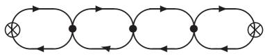
Figure 2: The bubble sum producing meson poles.

produces meson poles. The model with the parameters fitted in Bijnens:1992uz ; Bijnens:1995ww has a constituent quark mass of $M_{Q}=263$ MeV. It has a number decent matchings to QCD short distance, e.g. for $\Pi_{V}-\Pi_{A}$ but fails in others and it always generates a vector meson dominance (VMD) type of behaviour in couplings to external photons. Processes are constructed by one-loop “vertices” coupled together with bubble chain “propagators.” The relevant diagrams for HLbL are depicted in Fig. 3. Note that the exhange includes both the so-called pole and off-shell parts as calculated within the model. The vertices have also a nontrivial momentum dependence.

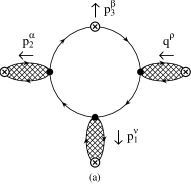
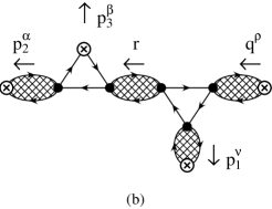
Figure 3: The two calsses of diagrams contributing to HLbL in the ENJL model. The crossed regions indicate the bubble sum “propagators.” (a) Quark-loop type (b) Resonance exchange type

4 $\pi^{0}$-exchange

The single largest numerical contribution is given by “$\pi^{0}$” exchange, depicted in Fig. 4.

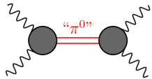
Figure 4: The $\pi^{0}$ exchange contribution. The blobs and the propagator need modeling.

The blobs need modeling and the propagator in the ENJL model also has corrections to the $1/(p^{2}-m_{\pi^{0}}^{2})$. The pointlike vertex has a logarithmic divergence which is uniquely predicted Knecht:2001qg ; RamseyMusolf:2002cy . The VMD form-factor in the $\pi^{0}\gamma^{*}\gamma^{*}$ form-factor, the blobs, were modeled in Bijnens:1995xf with a variety of form-factors and as a function of the cut-off $\Lambda$ (corrected for the overall sign error discovered by Knecht:2001qf ).

Table 1: The $\pi^{0}$ exchange results of Bijnens:1995xf .

	$a_{\mu}\times 10^{10}$
$\Lambda$	Point-	ENJL-	Point-	Transv.	CELLO-
GeV	like	VMD	VMD	VMD	VMD
0.5	4.92(2)	3.29(2)	3.46(2)	3.60(3)	3.53(2)
0.7	7.68(4)	4.24(4)	4.49(3)	4.73(4)	4.57(4)
1.0	11.15(7)	4.90(5)	5.18(3)	5.61(6)	5.29(5)
2.0	21.3(2)	5.63(8)	5.62(5)	6.39(9)	5.89(8)
4.0	32.7(5)	6.22(17)	5.58(5)	6.59(16)	6.02(10)

We took the form-factor that was made to fit the then existing data integrated up to 2 GeV as our main result with a guesstimate of the error. This result was in quite good agreement with Hayakawa:1996ki which used the pointlike-VMD approach. This contribution has since been reevaluated many times using different models and approaches. A partial list is:
BPP Bijnens:1995xf : $5.9(0.9)\times 10^{-10}$
Nonlocal quark model Dorokhov:2008pw : $6.27\times 10^{-10}$
DSE (Dyson-Schwinger modeling)Goecke:2010if : $5.75\times 10^{-10}$
LMD+V Knecht:2001qf : $(5.8-6.3)\times 10^{-10}$
Formfactor inspired by AdS/QCD Cappiello ; Cappiello:2010uy : $6.54\times 10^{-10}$
Chiral Quark Model Greynat:2012ww : $6.8\times 10^{-10}$
Constraint via magnetic susceptibility Nyffeler:2009tw : $7.2\times 10^{-10}$
$VV^{\prime}P$ model Roig:2014uja : $6.66\times 10^{-10}$
All of these are in reasonable agreement, within the errors. Future improvements will come when more experimental results are included as discussed in the talk by Nyffeler Nyffeler .

Two more comments are needed. The above numbers are for the $\pi^{0}$. One needs to take into account the $\eta$ and $\eta^{\prime}$ exchange as well. The latter is enhanced due to the charge combinations in the $\eta^{\prime}\gamma^{*}\gamma^{*}$ vertex. In large $N_{c}$ models like the ENJL model, the pseudoscalar spectrum is not like QCD, one has a $\pi^{0}$, a $\tilde{\pi}$ ($\bar{u}u+\bar{d}d$ quark content) and a $\pi_{s}$ ($\bar{s}s$). The $\tilde{\pi}$ has the same mass as the $\pi^{0}$ and due to the quark charges is contributes $25/9$ times the $\pi^{0}$ contribution. Lattice QCD calculations with only connected diagrams included will have the $\tilde{\pi}$ contribution as well so there will be an unphysical enhancement compared to the QCD result for the pseudoscalar exchange part. In Bijnens:1995xf we used pointlike-VMD to estimate the ratio of $\pi^{0},\eta,\eta^{\prime}$ contributions as $5.58,1.38,1.04$. Models that include large $N_{c}$-breaking effects and fit the mixings to data typically end up with very similar numbers. The total pseudoscalar exchange contribution I thus estimate to be

$$a_{\mu}^{PS}=(8-10)\times 10^{-10}$$ (3)

An example of a specific calculation is the AdS/QCD result of $a_{\mu}^{PS}=10.7\times 10^{-10}$ Hong:2009zw which also includes excited pseudoscalars.

The other comment is that the short-distance behaviour of the four-point function is known in several limits. In particular when $P_{1}^{2}\approx P_{2}^{2}\gg Q^{2}$ the four point function is related to the axial-vector-vector-vector three-point function Melnikov:2003xd . This three point function has a number of exact properties in QCD and we thus know how it behaves. The above models for $\pi^{0}$-exchange do not exhibit this behaviour. It can be implemented via making one of the blobs in Fig. 4 pointlike Melnikov:2003xd and one then obtains $7.7\times 10^{-10}$ for the $\pi^{0}$-exchange contribution. Plots how this affects the contribution of different momentum regions are in Bijnens:2007pz . The above behaviour of the four-point function must be obeyed in a full calculation, however whether one implements it via $\pi^{0}$-exchange is a choice. Models incorporating a short-distance quark-loop contribution have the short-distance part of this included Bijnens:2007pz ; Dorokhov:2008pw . One can see this when comparing quark-loop plus pseudo-scalar exchange of Bijnens:1995xf with pseudo-scalar exchange of Melnikov:2003xd .

5 Quark-loop

The pure quark-loop contribution with a constant mass is known analytically. One of the surprises is that it converges rather slowly. A significant portion is from high momentum regions. With a constituent quark mass of 300 MeV and a cut-off of 1(2) GeV 50(25)% of the full contribution is still missing. A more visual illustration of this is the plot of $a_{\mu}^{LLQ}$ defined in (2) of this contribution. The contribition is plotted in Fig. 5 as a function of $P_{1}$ and $Q$ for several ratios of $P_{2}/P_{1}$. The volume under the curve is proportional to $a_{\mu}$. The contribution peaks for $P_{1}\approx P_{2}\approx Q$ and around 1 GeV.

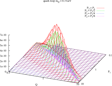
Figure 5: The quantity $a_{\mu}^{LLQ}$ defined in (2) as a function of $P_{1}$ and $Q$ for several ratios $P_{1}/P_{1}$. The lines indicate the surface.

In Bijnens:1995xf we used the ENJL up to a cut-off $\Lambda$ and added a short-distance quark-loop where we used the quark-mass $M_{H}=\Lambda$ as a lower cut-off. The estimate used by HKS was a quark-loop damped by VMD factors in the photon legs. The results are given in Tab. 2. Notice especially the stability when we add the ENJL and the short-distance contribution in the region $\Lambda=1$-8 GeV.

Table 2: The quark-loop contribution with VMD damping, the ENJL model and with a heavy quark mass as cut-off. The numbers are $a_{\mu}\times 10^{10}$.

Cut-off				sum
$\Lambda$			mass-	ENJL
GeV	VMD	ENJL	cut	masscut
0.5	0.48	0.78	2.46	3.2
0.7	0.72	1.14	1.13	2.3
1.0	0.87	1.44	0.59	2.0
2.0	0.98	1.78	0.13	1.9
4.0	0.98	1.98	0.03	2.0
8.0	0.98	2.00	.005	2.0

The conclusion is that the quark-loop is about $2\times 10^{-10}$. In the ENJL model the quark-loop and scalar exchange are needed together to have correct chiral symmetry. The sum of both is very similar to the quark-loop estimate of HKS.

There are a number of estimates of the quark-loop that lead to much larger numbers. These have all in common that there is a momentum region with a fairly small (constituent) quark mass that is not shielded by a VMD-like mechanism. The most prominent example of this is the DSE estimate of Goecke:2012qm $10.7(0.2)\times 10^{-10}$. The present status of this calculation is given in Eichmann:2014ooa . It not yet a full calculation but includes an estimate of some of the missing parts. This DSE model describes a lot of low-energy phenomenology in a way very similar to the ENJL model. I am quite puzzled by the difference in results.

Similar size numbers are obtained in models with a low constituent quark mass where no VMD-like dynamical effects are included. Examples are the nonlocal chiral quark model Dorokhov:2015psa with $11.0(0.9)\times 10^{-10}$ and a number of estimates within the chiral quark model $(7.6-8.9)\times 10^{-10}$ Greynat:2012ww , $(11.8-14.8)\times 10^{-10}$ Boughezal:2011vw and $(7.6-12.5)\times 10^{-10}$Masjuan:2012qn . The interpretation varies from an estimate to the full HLbL or just a part that needs to be added to other contributions.

6 Scalar exchange

The estimate of the scalar exchange contribution in the ENJL model is $-0.7\times 10^{-10}$. Similar size estimates have been obtained when exchanging a sigma-like particle. It should be pointed out that the scalar in the ENJL model has a phenomenology similar to the sigma but is quite a different underlying object.

A problem here is to distinguish scalar exchange from two-pion or pion-loop contributions. This is one of the areas where the method of Procura ; Colangelo:2014dfa will allow progress.

7 $a_{1}$-exchange

The exchange of axial vectors in the ENJL model was estimated in Bijnens:1995xf to be about $0.6\times 10^{-10}$, but due to the high mass involved, even with a cut-off of 2 GeV only half the contribution was there. The ENJL part also includes some pseudo-scalar meson exchange due to the structure of the calculation.

Axial-vector meson exchange in a more phenomenological way was done using two multiplets in Melnikov:2003xd who obtained $2.2\times 10^{-10}$. It was later found that when correct antisymmetrization is included, this becomes smaller by a significant factor and is again in the ballpark of the ENJL result. This was noticed by F. Jegerlehner. He obtains about $(0.76\pm 0.27)\times 10^{-10}$ for the axial-vector exchange Jegerlehner1 ; Jegerlehner2 . The evaluation of Pauk:2014rta is also in reasonable agreement with the ENJL estimate.

8 $\pi$-loop

The $\pi$-loop contribution to the four-point function is depicted in Fig. 6.

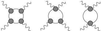
Figure 6: The charged pion loop contribution.

The leftmost diagram is the naive one, the other two are required by gauge-invariance. In more general models also a diagram with three photons in one vertex and one with all four in the same vertex might be needed. These have been included in the calculations mentioned below when needed.

The simplest model is a point-like pion or scalar QED (sQED). This gives a contribution of about $-4\times 10^{-10}$.

The single photon vertex is in all determinations used as including the pion form-factor. For this one can use either the VMD expression or a more model/experimental inspired version. For the $\pi\pi\gamma^{*}\gamma^{*}$ vertex there were originally two main approaches used, full VMD (BPP) and the hidden local symmetry model with vector mesons (HKS). The former is essentially using sQED and putting a VMD-like form-factor in all the photon legs. This was proven to be a consistent procedure in Bijnens:1995xf . We obtained there a result of $-1.9\times 10^{-10}$ using an ENJL inspired pion form-factor. Using a simple VMD typically gives about $-1.6\times 10^{-10}$. This version is exactly what is called the model-independent part of the two-pion contribution in Procura ; Colangelo:2014dfa ; Colangelo:2014pva . The reason for the lower number compared to the point-like pion loop is obvious in Fig. 7 where we show $a_{\mu}^{LLQ}$ of (2) as a function of $P_{1}=P_{2}$ and $Q$.

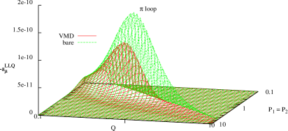
Figure 7: The momentum dependence of the pion loop contribution. Plotted is $a_{\mu}^{LLQ}$ of (2) as a function of $P_{1}=P_{2}$ and $Q$. Top surface: sQED, bottom surface:full VMD.

HKS Hayakawa:1995ps ; Hayakawa:1996ki used a different approach. Due to the then existing arguments against full VMD they used the hidden local symmetry model with only vector mesons (HLS) and obtained $-0.45\times 10^{-10}$. The difference between this and the previous numbers was the reason for the large error quoted on the pion-loop. This difference was rather puzzling, one reason could be that the HLS model does not have the correct QCD short distance constraint when looking at the two-photon vertex with the same and large virtuality for both photons, the full VMD model has the correct behaviour. This version of the HLS model also does not give a finite prediction for the $\pi^{+}$-$\pi^{0}$ mass difference. The reason for the large numerical difference is indeed the short distance behaviour. The low momentum behviour is very close but the negative

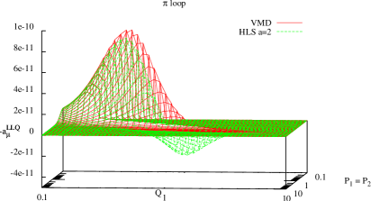
Figure 8: $-a_{\mu}^{LLQ}$ of (2) as a function of $P_{1}=P_{2}$ and $Q$. Top surface: full VMD, bottom surface: HLS.

contribution above 1 GeV, clearly visible in Fig. 8, is the main reason for the difference JBJR ; Bijnens:2012an . A comparison as a function of the cut-off can be found in Abyaneh:2012ak . In fact, using the HLS with an unphysical value of the parameter $a=1$, which then satisfies the abovementioned short-distance constraint gives very similar numbers as full VMD. This is shown in Fig. 9

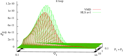
Figure 9: The momentum dependence of the pion loop contribution. $-a_{\mu}^{LLQ}$ of (2) as a function of $P_{1}=P_{2}$ and $Q$. Top surface: HLS a=1, bottom surface: full VMD.

From this we conclude that a number in the range $-(1.5$-$1.9)\times 10^{-10}$ is more appropriate with an error of half to 1/3 that.

More recently, it was pointed out that the effect of pion polarizability was neglected in these calculations and a first estimate of this effect given using the Euler-Heisenberg four photon effective vertex produced by pions Engel:2012xb within Chiral Perturbation Theory. This approximation is only valid below the pion mass. In order to check the size of the pion radius effect and the polarizability we have implemented the low energy part of the four-point function and computed $a_{\mu}^{LLQ}$ for these cases. Partial results are in Bijnens:2012an ; Abyaneh:2012ak . Full results will be published in JBJR . The effect of the charge radius is shown in Fig. 10 compared to the VMD, notice the different momentum scales compared to the earlier figures. As expected, the charge radius effect is included in the VMD result since the latter gives a good description of the pion form-factor.

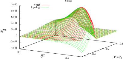
Figure 10: $-a_{\mu}^{LLQ}$ of (2) as a function of $P_{1}=P_{2}$ and $Q$. Top surface: full VMD, bottom surface: ChPT with $L_{9}=-L_{10}$ so the charge radius is included but no polarizability.

Including the effect of the polarizability can be done in ChPT by using experimentally determined values for $L_{9}$ and $L_{10}$. The latter can be determined from $\pi^{+}\to e\nu\gamma$ or the hadronic vector two-point functions. Both are in good agreement and lead to a prediction of the pion polarizability confirmed by the compass experiment Adolph:2014kgj . The effect of including this in ChPT on $a_{\mu}^{LLQ}$ is shown in Fig. 11 JBJR ; Bijnens:2012an ; Abyaneh:2012ak . An increase of 10-15% over the VMD estimate can be seen.

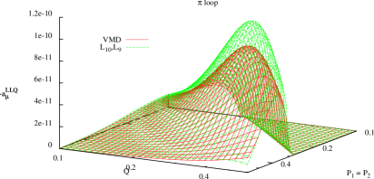
Figure 11: $-a_{\mu}^{LLQ}$ of (2) as a function of $P_{1}=P_{2}$ and $Q$. Bottom surface: full VMD, top surface: ChPT with $L_{9}\neq-L_{10}$ so the charge radius and the polarizability are included.

ChPT at lowest order or $p^{4}$ for $a_{\mu}$ is just the pointlike pion loop or sQED. At NLO pion exchange with pointlike vertices and the pionloop calculated at NLO in ChPT are needed. Both gives divergent contributions to $a_{\mu}$, so pure ChPT is of little use in predicting $a_{\mu}$. If we want to see the full effect of the polarizability we need to include a model that can be extended all the way, or at least to a cut-off of about 1 GeV. For the approach of Engel:2012xb this was done in Engel:2013kda by including a propagator description of $a_{1}$ and choosing it such that the full contribution of the pion-loop to $a_{\mu}$ is finite. They obtained a range of $-(1.1$-$7.1)\times 10^{-10}$ for the pion-loop contribution. I find this range much too broad. One reason is that the range of polarizabilities used in Engel:2013kda is simply not compatible with ChPT. The pion polarizability is an observable where ChPT should work and indeed the convergence is excellent. The ChPT prediction has also recently been confirmed by experiment. Our work discussed below indicates that $-(2.0\pm 0.5)\times 10^{-10}$ is a more appropriate range for the pion-loop contribution.

The work described below will be publsihed in JBJR . Preliminary results have been reported at several conferences, see e.g. Amaryan:2013eja ; Benayoun:2014tra and will be fully published in JBJR . The polarizability comes from $L_{9}+L_{10}$ in ChPT. Using Ecker:1988te , we notice that the polarizability is produced by $a_{1}$-exchange depicted in Fig. 12. This is depicted pictorially in the left diagram of Fig. 12.

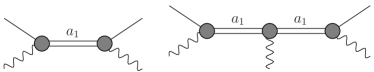
Figure 12: Left: the $a_{1}$-exchange that produces the pion polarizability. Right: an example of a diagram that is required by gauge invariance.

However, once such an exchange is there, diagrams like the right one in Fig. 12 lead to effective $\pi\pi\gamma\gamma\gamma$ vertices and are required by electromagnetic gauge invariance. This was done in Engel:2013kda via the propagator modifications. We deal with them via effective Lagrangians incorporating vector and axial-vector mesons.

If one looks at Fig. 12 one could raise the question “Is including a $\pi$-loop but no $a_{1}$-loop consistent?” The answer is yes with the following argument. We can fisrt look at a tree level Lagrangian including pions $\rho$ and $a_{1}$. We then integrate out the $\rho$ and $a_{1}$ and calculate the one-loop pion diagrams wth the resulting Lagrangian. In the diagrams of the original lagrangian this corresponds to only including loops with at least one pion propagator present. Numerical results for cases including full $a_{1}$ loops are presented as well below and in JBJR . As a technicality, we use anti-symmetric vector fields for the vector and axial-vector mesons. This avoids complications due to $\pi$-$a_{1}$ mixing. We add vector $V_{\mu\nu}$ and axial-vector $A_{\mu\nu}$ nonet fields. The kinetic terms are given by Ecker:1988te

$$-\frac{1}{2}\left\langle\nabla^{\lambda}V_{\lambda\mu}\nabla_{\nu}V^{\nu\mu}-\frac{M_{V}^{2}}{2}V_{\mu\nu}V^{\mu\nu}\right\rangle+V\leftrightarrow A\,.$$ (4)

First we add the terms that contribute to the $L_{i}$ Ecker:1988te

$$\frac{F_{V}}{2\sqrt{2}}\left\langle f_{+\mu\nu}V^{\mu\nu}\right\rangle+\frac{iG_{V}}{\sqrt{2}}\left\langle V^{\mu\nu}u_{\mu}u_{\nu}\right\rangle+\frac{F_{A}}{2\sqrt{2}}\left\langle f_{-\mu\nu}A^{\mu\nu}\right\rangle$$ (5)

with $L_{9}=\frac{F_{V}G_{V}}{2M_{V}^{2}}$, $L_{10}=-\frac{F_{V}^{2}}{4M_{V}^{2}}+\frac{F_{A}^{2}}{4M_{A}^{2}}$. The Weinberg sum rules imply in the chiral limit $F_{V}^{2}=F_{A}^{2}+F^{2}_{\pi}$, $F_{V}^{2}M_{V}^{2}=F_{A}^{2}M_{A}^{2}$ and requiring VMD behaviour for the pion form-factor $F_{V}G_{V}=F^{2}_{\pi}$.

First, look at the model with only $\pi$ and $\rho$. The one-loop contributions to $\Pi^{\rho\nu\alpha\beta}$ are not finite. They were also not finite for the HLS model of HKS, but the relevant $\delta\Pi^{\rho\nu\alpha\beta}/\delta p_{3\lambda}$ was. However, in the present model it is only finite for $G_{V}=F_{V}/2$ and then the result for $a_{\mu}$ is identical to the HLS model. The same comments as made for the HLS model thus also apply.

Next we do add the $a_{1}$ and require $F_{A}\neq 0$. After a lot of work we find that $\delta\Pi^{\rho\nu\alpha\beta}/\delta p_{3\lambda}|_{p_{3}=0}$ is finite only for $G_{V}=F_{V}=0$ and $F_{A}^{2}=-2F_{\pi}^{2}$ or, if including a full $a_{1}$-loop $F_{A}^{2}=-F_{\pi}^{2}$. These solutions are clearly unphysical. We then add all $\rho a_{1}\pi$ vertices given by

$$\lambda_{1}\left\langle\left[V^{\mu\nu},A_{\mu\nu}\right]\chi_{-}\right\rangle+\lambda_{2}\left\langle\left[V^{\mu\nu},A_{\nu\alpha}\right]{h_{\mu}}^{\nu}\right\rangle$$

$$+\lambda_{3}\left\langle i\left[\nabla^{\mu}V_{\mu\nu},A_{\nu\alpha}\right]u_{\alpha}\right\rangle+\lambda_{4}\left\langle i\left[\nabla_{\alpha}V_{\mu\nu},A_{\alpha\nu}\right]u^{\mu}\right\rangle$$

$$+\lambda_{5}\left\langle i\left[\nabla^{\alpha}V_{\mu\nu},A_{\mu\nu}\right]u_{\alpha}\right\rangle+\lambda_{6}\left\langle i\left[V^{\mu\nu},A_{\mu\nu}\right]{{f_{-}}^{\alpha}}_{\nu}\right\rangle$$

$$+\lambda_{7}\left\langle iV_{\mu\nu}A^{\mu\rho}{A^{\nu}}_{\rho}\right\rangle\,.$$ (6)

These are not all independent due to the constraints on $V_{\mu\nu}$ and $A_{\mu\nu}$ Leupold , there are three relations. After a lot of work JBJR we found that no solutions with $\delta\Pi^{\rho\nu\alpha\beta}/\delta p_{3\lambda}|_{p_{3}=0}$ exists except those already obtained without $\Lambda_{i}$ terms. The same conclusions holds if we look at the combination that shows up in the integral over $P_{1}^{2},P_{2}^{2},Q^{2}$. We thus find no reasonable model that has a finite prediction for $a_{\mu}$ for the pion-loop including $a_{1}$. If we choose the parameters as fixed by the Weinberg sum rules and the VMD behaviour of the pion-form factor we obtain $-a_{\mu}^{LLQ}$ as shown in Fig. 13.

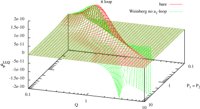
Figure 13: $-a_{\mu}{LLQ}$ as defined in (2) as a function of $P_{1}=P_{2}$ and $Q$ with $a_{1}$ but no full $a_{1}$-loop. Parameters determined by the Weinberg sum rules.

Adding a full $a_{1}$-loop changes the plot only marginally. As long as we require the correct polarizability and a VMD-like form-factor behaviour, the plots look quite similar for all cases below 1 GeV. The integrated value up to $\Lambda$ for a number of cases is hown in Fig. 14.

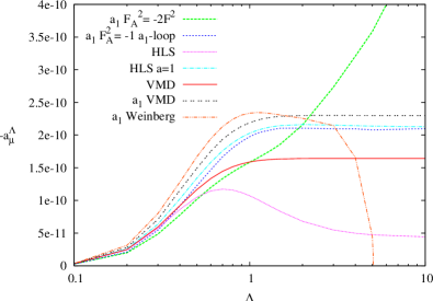
Figure 14: $-a_{\mu}$ using a variety of models for the pion loop as a functoin of $\Lambda$, the cut-off on the photon momenta.

We see that all models end up with a value of $a_{\mu}=-(2.0\pm 0.5)\times 10^{-10}$ when integrated up-to a cut-off of order 1-2 GeV. We conclude that that is a resonable estimate for the pion-loop contribution.

9 Conclusions

The present number for the HLbL contribution to the muon anomaly, $a_{\mu}=(g_{\mu}-2)/2$, is $(11\pm 4)$ or $(10.5\pm 2.6)\times 10^{-10}$ Bijnens:2007pz ; Prades:2009tw ; Jegerlehner:2009ry depending somewhat on which error estimates and which contributions are taken into account. In this talk I have given an overview of a number of model estimates with the emphasis on my old work Bijnens:1995cc ; Bijnens:1995xf ; Bijnens:2001cq as well as a number of newer developments. For the latter I have spent quite some time on our reevaluation of the pion loop contribution JBJR ; Bijnens:2012an ; Abyaneh:2012ak ; Amaryan:2013eja ; Benayoun:2014tra , as well as given a number of arguments why the HLS number of Hayakawa:1995ps ; Hayakawa:1996ki should be considered obsolete. The conclusion is that the pion-loop contributes with $-(2.0\pm 0.5)\times 10^{-10}$.

One of the remaining problems in the model approach is that the class of models with an “unshielded” quark-loop at relatively low-energies for the photns tend to obtain larger numbers. Whether this is a real phenomenon or not is a question which needs to be settled. My own opion there is that I see no counterpart of it in $\gamma\gamma\to$ hadrons at low to intermediate energies beyond the already included single meson and two-pion exchanges.

For contributions of different mechanisms, progress can be expected both from the dispersive approaches mentioned and experiment restricting the couplings of off-shell or virtual photons to meson that go into the modeling. Alternatively, a full new model calculation that includes phenomenology beyond what the ENJL does, is very desirable. For more deatils about the other approaches and the lattice I refer to the other talks at this conference.

References

- (1) K. Melnikov, Theory review on the muon g-2
- (2) M. Knecht, Perspectives on the hadronic contribution to the muon g-2
- (3) M. Procura, Recent developments in the calculation of the hadronic light-by-light contribution to the muon g-2
- (4) L. Capiello, What does holographic QCD predicts for the light-by-light scattering contribution to
- (5) D. Greynat, Hadronic contributions to the muon anomaly in the Constituent Chiral Quark Model
- (6) A. Nyffeler, On the precision of a data-driven estimate of the pseudoscalar-pole contribution to hadronic light-by-light scattering in the muon g-2
- (7) C. Lehner, Hadronic light-by-light contribution to from lattice QCD
- (8) M. Vanderhaeghen (by proxy due to a Lufthansa strike), Hadronic Light by Light corrections to (g-2)
- (9) G. W. Bennett et al. [Muon g-2 Collaboration], Phys. Rev. D 73, 072003 (2006) [hep-ex/0602035].
- (10) J. Bijnens and J. Prades, Mod. Phys. Lett. A 22, 767 (2007) [hep-ph/0702170].
- (11) J. Prades, E. de Rafael and A. Vainshtein, “Hadronic Light-by-Light Scattering Contribution to the Muon Anomalous Magnetic Moment,” (Advanced series on directions in high energy physics. 20) [arXiv:0901.0306 [hep-ph]].
- (12) F. Jegerlehner and A. Nyffeler, Phys. Rept. 477, 1 (2009) [arXiv:0902.3360 [hep-ph]].
- (13) J. Bijnens, E. Pallante and J. Prades, Phys. Rev. Lett. 75, 1447 (1995) [Phys. Rev. Lett. 75, 3781 (1995)] [hep-ph/9505251].
- (14) J. Bijnens, E. Pallante and J. Prades, Nucl. Phys. B 474, 379 (1996) [hep-ph/9511388].
- (15) J. Bijnens, E. Pallante and J. Prades, Nucl. Phys. B 626, 410 (2002) [hep-ph/0112255].
- (16) E. de Rafael, Phys. Lett. B 322, 239 (1994) [hep-ph/9311316].
- (17) M. Hayakawa, T. Kinoshita and A. I. Sanda, Phys. Rev. Lett. 75, 790 (1995) [hep-ph/9503463].
- (18) M. Hayakawa, T. Kinoshita and A. I. Sanda, Phys. Rev. D 54, 3137 (1996) [hep-ph/9601310].
- (19) M. Hayakawa and T. Kinoshita, Phys. Rev. D 57, 465 (1998) [Phys. Rev. D 66, 019902 (2002)] [hep-ph/9708227].
- (20) G. Eichmann, C. S. Fischer, W. Heupel and R. Williams, arXiv:1411.7876 [hep-ph].
- (21) J. Bijnens and J. Relefors, work in progress.
- (22) M. Knecht and A. Nyffeler, Phys. Rev. D 65, 073034 (2002) [hep-ph/0111058].
- (23) J. Bijnens, C. Bruno and E. de Rafael, Nucl. Phys. B 390, 501 (1993) [hep-ph/9206236].
- (24) J. Bijnens, Phys. Rept. 265, 369 (1996) [hep-ph/9502335].
- (25) M. Knecht, A. Nyffeler, M. Perrottet and E. de Rafael, Phys. Rev. Lett. 88, 071802 (2002) [hep-ph/0111059].
- (26) M. J. Ramsey-Musolf and M. B. Wise, Phys. Rev. Lett. 89, 041601 (2002) [hep-ph/0201297].
- (27) A. E. Dorokhov and W. Broniowski, Phys. Rev. D 78, 073011 (2008) [arXiv:0805.0760 [hep-ph]].
- (28) T. Goecke, C. S. Fischer and R. Williams, Phys. Rev. D 83, 094006 (2011) [Phys. Rev. D 86, 099901 (2012)] [arXiv:1012.3886 [hep-ph]].
- (29) L. Cappiello, O. Cata and G. D’Ambrosio, Phys. Rev. D 83, 093006 (2011) [arXiv:1009.1161 [hep-ph]].
- (30) D. Greynat and E. de Rafael, JHEP 1207, 020 (2012) [arXiv:1204.3029 [hep-ph]].
- (31) A. Nyffeler, Phys. Rev. D 79, 073012 (2009) [arXiv:0901.1172 [hep-ph]].
- (32) P. Roig, A. Guevara and G. LÃpez Castro, Phys. Rev. D 89, no. 7, 073016 (2014) [arXiv:1401.4099 [hep-ph]].
- (33) D. K. Hong and D. Kim, Phys. Lett. B 680, 480 (2009) [arXiv:0904.4042 [hep-ph]].
- (34) K. Melnikov and A. Vainshtein, Phys. Rev. D 70, 113006 (2004) [hep-ph/0312226].
- (35) T. Goecke, C. S. Fischer and R. Williams, Phys. Rev. D 87, no. 3, 034013 (2013) [arXiv:1210.1759 [hep-ph]].
- (36) A. E. Dorokhov, A. E. Radzhabov and A. S. Zhevlakov, Eur. Phys. J. C 75, no. 9, 417 (2015) [arXiv:1502.04487 [hep-ph]].
- (37) R. Boughezal and K. Melnikov, Phys. Lett. B 704, 193 (2014) [arXiv:1104.4510 [hep-ph]].
- (38) P. Masjuan and M. Vanderhaeghen, arXiv:1212.0357 [hep-ph].
- (39) G. Colangelo, M. Hoferichter, M. Procura and P. Stoffer, JHEP 1409, 091 (2014) [arXiv:1402.7081 [hep-ph]].
- (40) F. Jegerlehner, talk presented at the workshop on Hadronic contributions to the muon anomalous magnetic moment: strategies for improvements of the accuracy of the theoretical prediction, 1-5 April 2014, Waldthausen Castle near Mainz.
- (41) F. Jegerlehner, this conference.
- (42) V. Pauk and M. Vanderhaeghen, Eur. Phys. J. C 74, no. 8, 3008 (2014) [arXiv:1401.0832 [hep-ph]].
- (43) G. Colangelo, M. Hoferichter, B. Kubis, M. Procura and P. Stoffer, Phys. Lett. B 738, 6 (2014) [arXiv:1408.2517 [hep-ph]].
- (44) J. Bijnens and M. Z. Abyaneh, EPJ Web Conf. 37, 01007 (2012) [arXiv:1208.3548 [hep-ph]].
- (45) M. Z. Abyaneh, arXiv:1208.2554 [hep-ph].
- (46) K. T. Engel, H. H. Patel and M. J. Ramsey-Musolf, Phys. Rev. D 86, 037502 (2012) [arXiv:1201.0809 [hep-ph]].
- (47) C. Adolph et al. [COMPASS Collaboration], Phys. Rev. Lett. 114, 062002 (2015) [arXiv:1405.6377 [hep-ex]].
- (48) K. T. Engel and M. J. Ramsey-Musolf, Phys. Lett. B 738, 123 (2014) [arXiv:1309.2225 [hep-ph]].
- (49) K. Kampf et al., arXiv:1308.2575 [hep-ph].
- (50) M. Benayoun et al., arXiv:1407.4021 [hep-ph].
- (51) G. Ecker, J. Gasser, A. Pich and E. de Rafael, Nucl. Phys. B 321, 311 (1989).
- (52) S. Leupold, private communication.