Adiabatic electronic flux density: a Born-Oppenheimer Broken Symmetry ansatz

Abstract

The Born-Oppenheimer approximation leads to the counterintuitive result of a vanishing electronic flux density upon vibrational dynamics in the electronic ground state. To circumvent this long known issue, we propose using pairwise anti-symmetrically translated vibronic densities to generate a symmetric electronic density that can be forced to satisfy the continuity equation approximately. The so-called Born-Oppenheimer broken symmetry ansatz yields all components of the flux density simultaneously while requiring only knowledge about the nuclear quantum dynamics on the electronic adiabatic ground state potential energy surface. The underlying minimization procedure is transparent and computationally inexpensive, and the solution can be computed from the standard output of any quantum chemistry program. Taylor series expansion reveals that the implicit electron dynamics originates from non-adiabatic coupling to the explicit Born-Oppenheimer nuclear dynamics. The new approach is applied to the ${\rm H}_{2}^{+}$ molecular ion vibrating in its ${}^{2}\Sigma^{+}_{g}$ ground state. The electronic flux density is found to have the correct nodal structure and symmetry properties at all times.

I Introduction

Within the Born-Oppenheimer framework Born and Oppenheimer (1927), molecules are described as moving adiabatically on a potential energy landscape defined by the system electrons Eyring (1935); Evans and Polanyi (1935); Polanyi (1987). Quantitative knowledge of the electronic flux during molecular processes could lead to a deeper understanding of their underlying mechanisms. Interpreting the electronic density as a probability fluid, the flux of electrons is usually described as the amount of probability crossing dividing surfaces per unit time Mita (2001). As such, the electronic flux is defined from a scalar field, the electron flow, that can be reconstructed in principle from the time evolution of an experimentally observed electronic probability Dixit et al. (2012, 2013); Suominen and Kirrander (2014). This was already achieved experimentally for the nuclear density analogon Frohnmeyer and Baumert (2000); Ergler et al. (2006); Manz et al. (2013). From a theoretical perspective, the determination of electronic fluxes suffers from the requirement of defining dividing surfaces in nuclear configuration space, for which the definition of a partitioning scheme is not unique. This problem is also encountered in, e.g., the determination of individual atomic charges in molecules Fonseca Guerra et al. (2004), and it is exacerbated by the fact that nuclei are moving during the molecular process of interest and that their position is only defined as a quantum mechanical distribution, as opposed to a single point in nuclear configuration space.

To complement the information obtained from the electronic fluxes, the knowledge of the time-dependent electronic flux densities can significantly improve understanding of these processes at a microscopic level. The latter object corresponds to a vector field describing the instantaneous displacement of probability fluid elements at every point in electronic configuration space, and it does not rely on a particular nuclear spatial partitioning scheme. In conventional quantum molecular dynamics simulations, electrons are adiabatically separated from the motion of the nuclei because of their large mass mismatch. The solution to the Schrödinger equation leads to a real-valued, stationary electronic wavefunction for each given nuclear configuration. This has the unfortunate consequence of leading to a vanishing electronic flux density Schrödinger (1926). A workaround to this unphysical result can be obtained by means of a vibronic Born-Huang expansion Born and Huang (1954), where the nuclear dynamics is performed on multiple coupled potential energy surfaces simultaneously. Since the determination of the electronic flux density beyond the Born-Oppenheimer approximation are computationally demanding, only very few molecular systems, H${}_{2}^{+}$Paramonov (2005); Kono et al. (2006); Karr and Hilico (2006); Niederhausen et al. (2012); Ishikawa et al. (2012); Pérez-Torres (2013), H₂ Bubin et al. (2009); Chen and Anderson (1995), and H₂D⁺Mátyus et al. (2011); Mátyus and Reiher (2012), have been investigated up to date. Hence, new approximate schemes are required to overcome this problem.

A point of particular interest is that electronic flux densities computed using the Born-Huang ansatz reveal that the nuclear dynamics from which it emerges almost quantitatively follows the ground state molecular dynamics for small amplitude vibrations, contrary to the adiabatic Born-Oppenheimer picture. To circumvent this long known issue, a few workarounds have been proposed that suffer from various drawbacks. In the semi-classical coupled channels theory D. J. Diestler (2012); Diestler et al. (2012, 2013); Hermann et al. (2014), the electronic flux density strictly follows the nuclear motion, while the time-shift classical approach of Okayama and Takatsuka Okuyama and Takatsuka (2009) yields a complex-valued flux density. Other attempts at reducing the complete Schrödinger equation provide information about individual components of the flux density in the average field of the others Bredtmann et al. (2015). Perturbative approaches including the effect of multiple excited electronic states have also been put forward with various degree of success Nafie (1983); Patchkovskii (2012); Diestler (2013), but their framework departs from the Born-Oppenheimer picture.

In an attempt to reconcile the adiabatic approximation with the intuitive picture of electrons flowing along with the nuclear motion, we present an alternative ansatz correlating the electronic with the nuclear motion. Starting from the Liouville von Neumann equation for the evolution of the vibronic density matrix operator, we first reveal inconsistencies in the Born-Oppenheimer approximation. In order to rectify these, pairwise antisymmetric translation operators are introduced to shift the density matrix operator within the nuclear configuration space. Tracing out the nuclear degrees of freedom yields an electronic continuity equation stemming from a single reduced electronic density depending on a single parameter, the so-called correlation length. The continuity equation can thus be seen satisfied approximately by numerical optimization of a cost equation, for which a robust and computationally inexpensive implementation is obtained by means of Taylor series expansion. The method is applied to a first model system, the hydrogen molecular ion ${\rm H}_{2}^{+}$ vibrating in the electronic ground state ${}^{2}\Sigma^{+}_{g}$, for which non Born-Oppenheimer results are available Pérez-Torres (2013); Diestler et al. (2013).

II Theory

The object of our investigations, the electronic probability density, can be understood as a diagonal element of the reduced electron density matrix in the position representation. The latter can be obtained from the reduction of the total density operator, $\hat{\Theta}(t)$, which evolves according to the Liouville von Neumann equation

$$\frac{\partial}{\partial t}\hat{\Theta}(t)=-\frac{\imath}{\hbar}\left[\hat{H}_{\rm el}+\hat{T}_{\rm nuc},\hat{\Theta}(t)\right]$$ (1)

with the electronic Hamiltonian $\hat{H}_{\rm el}$ and the nuclear kinetic energy operator $\hat{T}_{\rm nuc}$. For a coherent vibronic system in a pure state, this density matrix operator $\hat{\Theta}(t)$ can be factorized as

$$\hat{\Theta}(t)=\left|\psi(t)\right\rangle\left\langle\psi(t)\right|.$$ (2)

Within the Born-Oppenheimer approximation, the system wavefunction $\left|\psi(t)\right\rangle$ is written as

$$\left|\psi(t)\right\rangle=\left|\varphi\right\rangle\left|\chi(t)\right\rangle,$$ (3)

with the time-dependent nuclear wavefunction $\left|\chi(t)\right\rangle$ and the time-independent electronic wavefunction $\left|\varphi\right\rangle$. The latter is defined by the time-independent electronic Schödinger Equation $\hat{H}_{\rm el}\left|\varphi\right\rangle=V_{\rm tot}\left|\varphi\right\rangle$. Here, the electronic Hamiltonian $\hat{H}_{\rm el}=\hat{T}_{\rm el}+\hat{V}_{\rm eff}$ refers to an effective one-electron operator in the spirit of the density functional theory, i.e., we define an effective potential energy operator $\hat{V}_{\rm eff}$ as a time-dependent multiplicative potential according to the Runge-Gross theorem Runge and Gross (1984).

The electronic probability density at an observation point $r$ can be defined by the trace over the nuclear contributions, here given in the position representation

$$\rho_{\rm el}(r,t) = \int{\rm d}Q\left\langle r,Q\right|\hat{\Theta}(t)\left|r,Q\right\rangle$$

$$= \int{\rm d}Q\left\langle r,Q\middle|\psi(t)\right\rangle\left\langle\psi(t)\middle|r,Q\right\rangle$$

$$= \int{\rm d}Q\,|\varphi(r;Q)|^{2}|\chi(Q,t)|^{2}.$$ (5)

Note that the nuclear wavefunction depends on time $t$ and the nuclear coordinate $Q$, and the electronic wavefunction depends on the electronic coordinate $r$ and parametrically on the nuclear coordinate $Q$.

II.1 Time evolution of the electron density within the Born-Oppenheimer approximation

To reveal a fundamental problem of the Born-Oppenheimer approximation, expressions for the time evolution of the electron density are deduced following two different routes: taking the time-derivative of the electronic density after reduction of the total density matrix [cf. Eq. (5)], or reducing the equations of motion after the applying the respective operators to the wavefunctions [cf. Eqs. (1) and (II)]. For clarity, only a system consisting of one effective nuclear coordinate $Q$ with mass $\mu_{Q}$ is considered throughout. The procedure can be easily extended to a higher dimensionality.

Based on Eq. (5), the time evolution of the electronic density can be written as

$$\frac{\partial}{\partial t}\rho_{\rm el}(r,t) =\frac{\partial}{\partial t}\int{\rm d}Q|\varphi(r;Q)|^{2}|\chi(Q,t)|^{2}$$ (6)

$$=\int{\rm d}Q|\varphi(r;Q)|^{2}\frac{\partial}{\partial t}\Big{(}|\chi(Q,t)|^{2}\Big{)}.$$

Using the time-dependent nuclear Schödinger equation,

$$\frac{\partial}{\partial t}\chi(Q,t) =-\frac{\imath}{\hbar}\big{(}\hat{T}_{\rm nuc}+V_{\rm tot}\big{)}\chi(Q,t),$$ (7)

the time derivative of the nuclear density leads to the nuclear continuity equation

$$\frac{\partial}{\partial t}|\chi(Q,t)|^{2} =\chi(Q,t)\frac{\partial}{\partial t}\chi^{\dagger}(Q,t)+\chi^{\dagger}(Q,t)\frac{\partial}{\partial t}\chi(Q,t)$$ (8)

$$=\frac{\imath\hbar}{2\mu_{Q}}\left(\chi^{\dagger}(Q,t)\nabla_{Q}^{2}\chi(Q,t)-{\rm c.c.}\right)$$

$$=-\nabla_{Q}\cdot\vec{j}_{\rm nuc},$$

where “c.c.“ stands for the complex conjugate and $\vec{j}_{\rm nuc}$ is the nuclear flux density. Inserting the result into Eq. (6) yields

$$\frac{\partial}{\partial t}\rho_{\rm el}(r,t) =-\int{\rm d}Q\Big{(}\nabla_{Q}|\varphi(r;Q)|^{2}\Big{)}\cdot\vec{j}_{\rm nuc}.$$ (9)

In deriving Eq. (9), the divergence theorem was applied to eliminate a vanishing contribution from the bound vibrational states. This electronic flow cannot be trivially expressed as the divergence of an electronic vector field, which is a requirement for formulating an expression for an electronic flux density.

As an alternative route starting from Eq. (II), the time evolution of the density matrix operator $\hat{\Theta}(t)$ is represented in the position representation using Eq. (1)

$$\frac{\partial}{\partial t} \rho_{\rm el}(r,t)=\int{\rm d}Q\left\langle r,Q\middle|\frac{\partial}{\partial t}\hat{\Theta}(t)\middle|r,Q\right\rangle$$ (10)

$$= -\frac{\imath}{\hbar}\int{\rm d}Q\Big{(}\left\langle r,Q\right|\hat{T}_{\rm el}\hat{\Theta}(t)\left|r,Q\right\rangle-\left\langle r,Q\right|\hat{\Theta}(t)\hat{T}_{\rm el}\left|r,Q\right\rangle+\left\langle r,Q\right|\hat{T}_{\rm nuc}\hat{\Theta}(t)\left|r,Q\right\rangle-\left\langle r,Q\right|\hat{\Theta}(t)\hat{T}_{\rm nuc}\left|r,Q\right\rangle$$

$$+\left\langle r,Q\right|\hat{V}_{\rm eff}\hat{\Theta}(t)\left|r,Q\right\rangle-\left\langle r,Q\right|\hat{\Theta}(t)\hat{V}_{\rm eff}\left|r,Q\right\rangle\Big{)}.$$

Here, the last line of Eq. (10) vanishes in the position representation, since $\hat{V}_{\rm eff}$ is a multiplicative operator. At this stage, the electronic density still obeys both the Liouville von Neumann and the total continuity equations, as no assumption on the dynamics nor the specific form of the density operator has been made. Utilizing the Born-Oppenheimer ansatz [cf. Eq. (3)] for a density matrix representing a system in a pure state yields a vanishing electron flow

$$\frac{\partial}{\partial t} \rho_{\rm el}(r,t)=-\frac{\imath}{\hbar}\int{\rm d}Q|\chi(Q,t)|^{2}\left\{\varphi(r;Q)\left(-\frac{\hbar^{2}}{2m_{e}}\vec{\nabla}_{e}^{2}\varphi(r;Q)\right)-\varphi(r;Q)\left(-\frac{\hbar^{2}}{2m_{e}}\vec{\nabla}_{e}^{2}\varphi(r;Q)\right)\right\}$$ (11)

$$-\frac{\imath}{\hbar}\int{\rm d}Q\left\{\varphi(r;Q)\chi^{\dagger}(Q,t)\left(-\frac{\hbar^{2}}{2\mu_{Q}}\nabla_{Q}^{2}\right)\Big{(}\varphi(r;Q)\chi(Q,t)\Big{)}-\varphi(r;Q)\chi(Q,t)\left(-\frac{\hbar^{2}}{2\mu_{Q}}\nabla_{Q}^{2}\right)\Big{(}\varphi(r;Q)\chi^{\dagger}(Q,t)\Big{)}\right\}$$

$$= ~{}\frac{\imath\hbar}{2\mu_{Q}}\int{\rm d}Q\,\nabla_{Q}\cdot\bigg{(}\varphi(r;Q)\chi^{\dagger}(Q,t)\nabla_{Q}\Big{(}\varphi(r;Q)\chi(Q,t)\Big{)}-{\rm c.c.}\bigg{)}$$

$$= ~{}0,$$

where $\vec{\nabla}_{e}$ denotes the gradient with respect to the electronic coordinates $r$ and $m_{e}$ refers to the electronic mass. The last line of Eq. (11) arises from the divergence theorem and is valid for bound vibrational states. Eq. (9) stands in strong contradiction to Eq. (11): although the time evolution of the a priori reduced electron density shows a non-vanishing flow, there is neither a flow, nor a flux density in Eq. (11). This implies that the reduced electron density in Eq. (9) does not implicitly satisfy the Liouville von Neumann equation. This is because the a priori reduced electron density matrix is real and does not represent a pure state density matrix anymore.

II.2 Breaking the symmetry in the equation of motions

In order to fix this contradiction, which was already recognized by others (cf. for example D. J. Diestler (2012); Diestler et al. (2012, 2013); Okuyama and Takatsuka (2009); :M:EFD_Manz; Nafie (1983); Patchkovskii (2012); Diestler (2013)), we propose to break the symmetry of the equations of motion. To this end, a translation operator with the following properties is introduced

$$U_{Q}\left|Q\right\rangle=\left|Q+\delta_{q}\right\rangle~{}; ~{}U_{Q}^{\dagger}\left|Q\right\rangle=\left|Q-\delta_{q}\right\rangle$$ (12)

$$U_{Q}^{\dagger}~{}U_{Q}= ~{}U_{Q}~{}U_{Q}^{\dagger}=1$$

and a correlated electron density is defined

$$\rho_{c}=\frac{1}{2}\left(\rho_{+}+\rho_{-}\right).$$ (13)

To simplify the notation, the coordinate dependence in all quantities is omitted, i.e., $\rho_{+}(r,t)\equiv\rho_{+}$, $\varphi(r;Q+\delta_{q})\equiv\varphi^{+\delta_{q}}$, and $\chi(Q+\delta_{q},t)\equiv\chi^{+\delta_{q}}$. Here, a symmetric electron density $\rho_{c}$ is recovered by summing over the pairwise antisymmetric densities $\{\rho_{+},~{}\rho_{-}\}$.

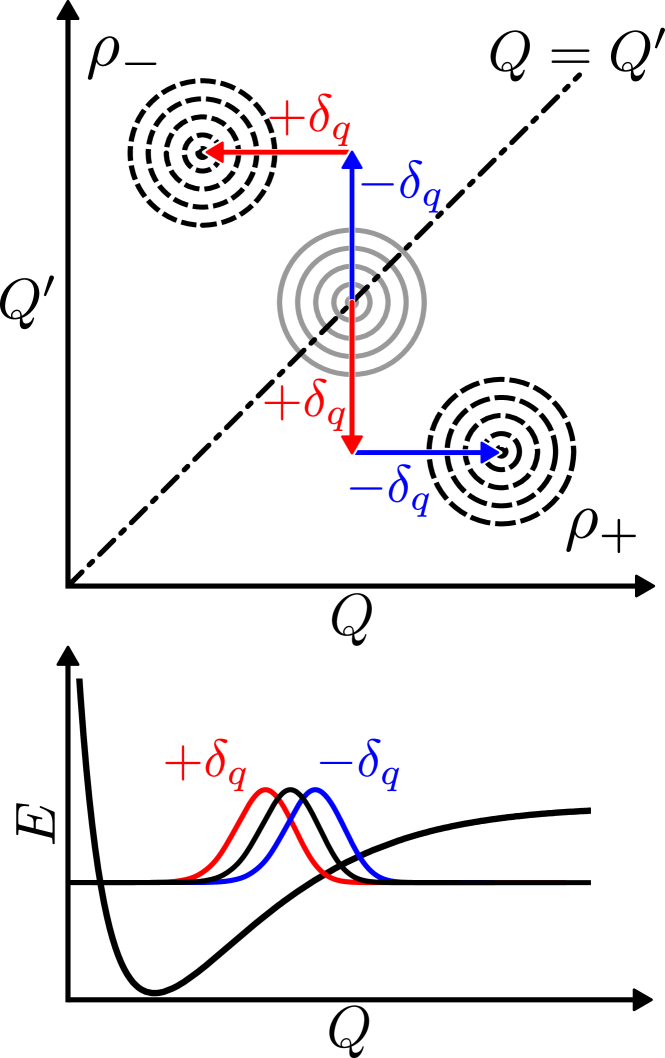
Figure 1: (Color online) Schematic representation of the Born-Oppenheimer broken symmetry ansatz. The bottom panel shows the two translated vibrational wavefunctions used to generate the broken symmetry densities. Top panel: a symmetric vibronic density is created by adding two pairwise antisymmetric densities with respect to the $Q=Q^{\prime}$ axis. The coordinate $Q^{\prime}$ is introduced to emphasize that two different translation are used in Eq. (13).

Positive displacement of the density along the nuclear coordinate $Q$ yields in the Born-Oppenheimer approximation

$$\rho_{+} =\int{\rm d}Q\left\langle r,Q\middle|U_{Q}\hat{\Theta}(t)U_{Q}\middle|r,Q\right\rangle$$ (14)

$$=\int{\rm d}Q\left\langle r,Q-\delta_{q}\middle|\hat{\Theta}(t)\middle|r,Q+\delta_{q}\right\rangle$$

$$=\int{\rm d}Q\left(\varphi^{-\delta_{q}}\varphi^{+\delta_{q}}\right)\left(\chi^{-\delta_{q}}\left(\chi^{+\delta_{q}}\right)^{\dagger}\right)$$

$$=\int{\rm d}Q\left(\varphi^{-\delta_{q}}\chi^{-\delta_{q}}\right)\left(\varphi^{+\delta_{q}}\chi^{+\delta_{q}}\right)^{\dagger},$$

and negative displacement results in $\rho_{-}$, which can be constructed analogously. The physical meaning given to $\delta_{q}$ is that of electron-nucleus correlation in nuclear configuration space, which we dub correlation length. Note that the transformation $U_{Q}\hat{\Theta}(t)U_{Q}$ is not unitary. The cartoon in the top panel of Fig. 1 illustrates how two pairwise antisymmetric densities created from the translation of vibronic wavefunctions at positive and negative correlation lengths $\delta_{q}$ can be used to generate a symmetric density. The vibrational part of the wavefunction and its translations are depicted in the bottom panel. The coordinate $Q^{\prime}$ in the top panel has been introduced to emphasize the fact that the density is computed as a product of two translated wavefunctions in opposite directions. By translating the density matrix $\langle r,Q^{\prime}|\hat{\Theta}(t)|r,Q\rangle$, spatial correlation within the nuclear configuration space is implicitly transfered from the off-diagonal elements of the vibronic density matrix to the diagonal elements of the reduced electron density matrix.

II.3 The correlated electronic continuity equation

Provided the broken symmetry reduced electronic density implicitly satisfies the Liouville von Neumann equation for the total density matrix, Eq. (1), the definition of an electron flow should be independent of the order in which the reduction procedure is performed [see Section II.1]. That is, substituting the correlated density for the electronic density in Eq. (5) and tracing out the nuclear degrees of freedom yields the following flow components

$$\frac{\partial}{\partial t}\rho_{c} =\frac{1}{2}\left(\frac{\partial}{\partial t}\rho_{+}+\frac{\partial}{\partial t}\rho_{-}\right)$$ (15)

$$\frac{\partial}{\partial t}\rho_{\pm} =\int{\rm d}Q\left(\varphi^{\mp\delta_{q}}\varphi^{\pm\delta_{q}}\right)\frac{\partial}{\partial t}\left(\chi^{\mp\delta_{q}}\left(\chi^{\pm\delta_{q}}\right)^{\dagger}\right)$$

Following the alternative route using the Liouville von Neumann equation as described in Eq. (10) and Eq. (11) with the correlated density yields a non-vanishing flow with components

$$\frac{\partial}{\partial t}\rho_{\pm} =-\frac{\imath\hbar}{2m_{e}}\vec{\nabla}_{e}\cdot\int{\rm d}Q$$ (16)

$$~{}\times\left(\varphi^{\mp\delta_{q}}\vec{\nabla}_{e}\varphi^{\pm\delta_{q}}-\varphi^{\pm\delta_{q}}\vec{\nabla}_{e}\varphi^{\mp\delta_{q}}\right)$$

$$~{}\times\left(\chi^{\mp\delta_{q}}\left(\chi^{\pm\delta_{q}}\right)^{\dagger}\right).$$

Note that two components appear naturally as the divergence of an electronic vector field which allows for a unique definition of the flux density as the sum of two broken symmetry terms

$$\vec{j}_{\pm} =\frac{\imath\hbar}{2m_{e}}\int{\rm d}Q\left(\varphi^{\mp\delta_{q}}\vec{\nabla}_{e}\varphi^{\pm\delta_{q}}-\varphi^{\pm\delta_{q}}\vec{\nabla}_{e}\varphi^{\mp\delta_{q}}\right)$$ (17)

$$\times\left(\chi^{\mp\delta_{q}}\left(\chi^{\pm\delta_{q}}\right)^{\dagger}\right)~{}.$$

Combining Eqs. (15) and (16) yields the following correlated electronic continuity equation

$$\frac{\partial}{\partial t}\rho_{c} =-\vec{\nabla}_{e}\cdot\vec{j}_{c}$$ (18)

$$\frac{1}{2}\left(\frac{\partial}{\partial t}\rho_{+}+\frac{\partial}{\partial t}\rho_{-}\right) =-\frac{1}{2}\left(\vec{\nabla}_{e}\cdot\vec{j}_{+}+\vec{\nabla}_{e}\cdot\vec{j}_{-}\right).$$

Since the validity of Eq. (18) depends only on a single control parameter, the correlation length $\delta_{q}$, it may be uniquely determined at each timestep by numerical minimization of the residual cost functional

$$\min_{\delta_{q}\in\Re}\left\|\frac{\partial}{\partial t}\rho_{c}+\vec{\nabla}_{e}\cdot\vec{j}_{c}\right\|_{2}.$$ (19)

We dub this procedure Born-Oppenheimer Broken Symmetry (BOBS) ansatz. It can be underlined that within the BOBS ansatz, the same correlated density yields an electron flow on the left and an electronic flux density on the right-hand-side of the electronic continuity equation Eq. (18).

II.4 Taylor series expansion

To reveal the physical origin of the flow and flux density in Eqs. (15-18), it is instructive to expand all terms using a Taylor series expansion around the point $Q$:

$$\varphi^{\pm\delta_{q}} =\varphi\pm\delta_{q}\left.\varphi^{\prime}\right|_{Q}+\frac{\delta_{q}^{2}}{2}\left.\varphi^{\prime\prime}\right|_{Q}\pm\dots$$ (20)

$$\chi^{\pm\delta_{q}} =\chi\pm\delta_{q}\left.\chi^{\prime}\right|_{Q}+\frac{\delta_{q}^{2}}{2}\left.\chi^{\prime\prime}\right|_{Q}\pm\dots$$

where an apostrophe abbreviates a nuclear derivative, e.g., $\chi^{\prime}=\partial\chi/\partial Q$. The series is expected to converge since the correlation length $\delta_{q}$ is small, as will be seen later.

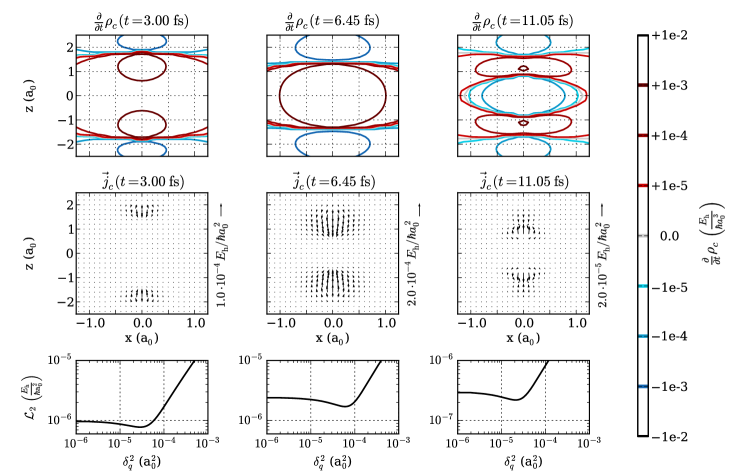
Figure 2: (Color online) Representative snapshots of the electron flow (top panel) and the electronic flux density (central panels) computed with the linearized BOBS ansatz [cf. Eqs. (LABEL:taylor_jc_left, 22)] for a vibrating hydrogen molecular ion ${\rm H}_{2}^{+}$ oriented along the $z$-axis. The results are plotted in the $xz$-plane for three different times within first half vibrational period: for $t=3\,{\rm fs}$ (left column), for $t=6.45\,{\rm fs}$ (middle column), and for $t=11.05\,{\rm fs}$ (right column). Note the logarithmic scale in the contour plots and the different scales in the vector plots. Bottom panels: Error of the correlated electronic continuity equation per grid point, $\mathcal{L}_{2}=\frac{1}{N}\big{\|}\frac{\partial}{\partial t}\rho_{c}+\vec{\nabla}_{e}\cdot\vec{j}_{c}\big{\|}_{2}$, as a function of the correlation length squared for the three selected snapshots.

Substituting Eq. (20) in Eq. (18), the left and the right-hand-side of the correlated continuity equation take the following form to second order

$$\frac{\partial}{\partial t}\rho_{c}=\int{\rm d}Q\left(\left|\varphi\right|^{2}+\delta_{q}^{2}\left(\varphi^{\prime\prime}\varphi-\varphi^{\prime}\varphi^{\prime}\right)\right)\frac{\partial}{\partial t}\left(\chi\chi^{\dagger}\right)$$ (21)

$$~{}+\frac{\delta_{q}^{2}}{2}\int{\rm d}Q\left|\varphi\right|^{2}\frac{\partial}{\partial t}\left(\chi^{\prime\prime}\chi^{\dagger}-2\chi^{\prime}\chi^{\prime\dagger}+\chi\chi^{\prime\prime\dagger}\right)+O\left(\delta_{q}^{4}\right)$$

and

$$-\vec{\nabla}_{e}\cdot\vec{j}_{c} =-\frac{\imath\hbar\delta_{q}^{2}}{m_{e}}\vec{\nabla}_{e}\cdot\int{\rm d}Q\left(\varphi\vec{\nabla}_{e}\varphi^{\prime}-\varphi^{\prime}\vec{\nabla}_{e}\varphi\right)$$ (22)

$$\times\left(\chi\chi^{\prime\dagger}-\chi^{\prime}\chi^{\dagger}\right)+O\left(\delta_{q}^{4}\right).$$

All electronic quantities appearing in the linearized BOBS ansatz remain real-valued and can be obtained from standard quantum chemistry programs. To zeroth order and/or for zero correlation length, the Born-Oppenheimer flow on the left-hand-side remains unchanged and the divergence of the flux density vanishes, leading to the aforementioned contradiction. Higher orders terms lead to a correction to the electron flow and the emergence of a new term on the right-hand-side that can be written as the divergence of a vector field. It is worth noticing that all odd terms in Eq. (20) vanish due to the symmetrization of the correlated density. Consequently, a Taylor series expansion to second order yields an error of order $O\big{(}\delta_{q}^{4}\big{)}$ on both sides of the equation.

The second order corrections to the electron flow, Eq. (LABEL:taylor_jc_left), and to the electronic flux density, Eq. (22), can be understood as non-adiabatic coupling elements. The first correction to the electron flow is the convolution of the nuclear flow with the nuclear spread of the electronic wavefunction, $(\varphi^{\prime\prime}\varphi-\varphi^{\prime}\varphi^{\prime})$, which is reminiscent of a Huang term. The second term is the convolution of the nuclear spread of the nuclear wavepacket, $(\chi^{\prime\prime}\chi^{\dagger}-2\chi^{\prime}\chi^{\prime\dagger}+\chi\chi^{\prime\prime\dagger})$, with the stationary ground state electronic density. The first term contributing to the electronic flux density involves mixed derivatives of the electronic and nuclear wavefunctions. Similar terms appear in first order time-dependent perturbation theory treatment of non-adiabatic couplings, which involved a transfer of momentum from nuclear to electronic degrees of freedom. In Eq. (22), the nuclear derivative of the ground state electronic wavefunction take place of the usual complex conjugate leading to a non-vanishing electron flow. Note that the antisymmetric nuclear term, $(\chi\chi^{\prime\dagger}-\chi^{\prime}\chi^{\dagger})$, yields a purely imaginary quantity, so that the total expression is real-valued.

It can be emphasized that, from a numerical perspective, Eqs. (LABEL:taylor_jc_left) and (22) are easy to handle since $\delta_{q}$ only appears as a multiplicative factor to the remaining terms. Nuclear derivatives of the electronic wavefunctions can thus be computed once prior to the dynamics, which significantly facilitates the determination of the optimal correlation length in Eq. (19). In the appendix, equations of motion for the correlated electron density in the basis of vibrational eigenstates of the electronic ground state are derived. These allow simplifying the evaluation of the nuclear wavefunction derivatives to that of the stationary vibrational eigenstates, which can be also evaluate once prior to the dynamical simulations. It is worth noting that, in this basis, the Born-Oppenheimer evolution of the wavepacket is known analytically at all times. Consequently, the BOBS ansatz is amenable to a simple, robust, and efficient numerical procedure which is in principle applicable to arbitrarily complex systems.

At this point, the similarities and differences between the BOBS ansatz and the complex ”time-shift“ flux proposed by Okuyama and Takatsuka Okuyama and Takatsuka (2009) should be compared. The latter is based on ab-initio molecular dynamics (AIMD), in which the nuclear positions follow classical trajectories. The authors break the symmetry of the equations of motion by ”translating“ the electronic wavefunctions against each other in the time domain, which amounts to a spatial translation in a classical AIMD context. The procedure yields a complex-valued flux density which disappears in the limit of vanishing time-shift, and the imaginary part is interpreted as an induced flux density. This is in stark contrast with the fully quantum mechanical BOBS procedure, where the nuclei are described by a wavefunction and are thus not localized. Further, since the dynamics is performed in the Born-Oppenheimer framework, a time-shift only affects the phase of the nuclear wavepacket. Consequently, a time-shifted quantum mechanical ansatz would lead to a vanishing flux density, as demonstrated in Section II.1. The spatial translation in the BOBS ansatz involves non-adiabatic coupling terms, and the resulting flow and associated flux density remain real-valued at all times.

III Computational details

As a model system, we consider the hydrogen molecular ion ${\rm H}_{2}^{+}$ vibrating in the electronic ground state ${}^{2}\Sigma^{+}_{g}$ oriented along the $z$-axis. The molpro software Werner et al. (2012) was used to compute the electronic ground state wavefunction $\varphi(r;Q)$ at the restricted open-shell Hartree Fock level of theory and using an aug-cc-pVTZ basis on all atoms Dunning (1989). The internuclear distance was scanned in the range $Q\in[0.4,18.06]\,{\rm a}_{0}$ at an equidistant interval of $\Delta Q=0.02\,{\rm a}_{0}$. Using the orbkit software Hermann et al. (2015), the ground state wavefunction and its analytical electronic derivatives were evaluated in the $xz$-plane, with $x=[-2.2,\,2.2]\,{\rm a_{0}}$, $z=[-3.5,\,3.5]\,{\rm a_{0}}$, and $\Delta x=\Delta z=0.1\,{\rm a_{0}}$. The nuclear derivatives of the ground state electronic wavefunction were determined numerically. The nuclear vibrational eigenstates $\chi_{n}(Q)$ and their derivatives were determined numerically using the wavepacket software Schmidt and Lorenz (2013).

In order to initiate a ground state dynamics, we chose the same initial conditions as J. F. Pérez-Torres Pérez-Torres (2013) and translated the vibrational ground state wavefunction $\chi_{0}$ by $+2.0\,{\rm a}_{0}$ to positive values of $Q$. The implementation of the correlated electronic continuity equation was achieved in the vibrational eigenstate representation, as described in Appendix A. The correlation length, $\delta_{q}$, was determined by minimization the $\mathcal{L}_{2}$-norm of the electronic continuity equation [cf. Eq. (19)] in its Taylor series form (linearized BOBS ansatz) with a Newton Conjugate-Gradient algorithm, as implemented in scipy Jones et al. (001). Minimization of the cost functional, Eq. (19), based on the non-linear Eqs. (16) and (15) yielded almost identical results as when using the second-order equations of motion and only the latter are reported below as the computationally substantially more efficient alternative. In order to obtain the shifted nuclear and electronic eigenfunctions for arbitrary values of $\delta_{q}$, the functions were interpolated along the nuclear configuration space $Q$ and evaluated the electronic wavefunction for each value of $\delta_{q}$ on the electronic grid $r$. This computationally very demanding task is solely required for the non-linear BOBS ansatz.

Figure 3: Detailed view of the symmetry properties of the flux density at the classical turning point, $t=11.05\,{\rm fs}$, at the topmost hydrogen atom (left panel) and close to the inversion center (right panel). The vector field is seen to be antisymmetric with respect to the molecular inversion center and the flux density is largest in the pointing towards of the nuclei.

IV Results and discussion

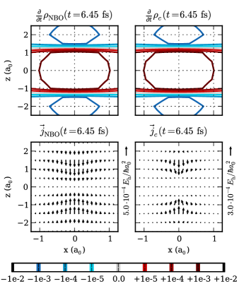
Figure 4: (Color online) Representative snapshot at $t=6.45\,{\rm fs}$ of the electron flow (top panels) and the electronic flux density (bottom panels) in the $xz$-plane for a vibrating hydrogen molecular ion ${\rm H}_{2}^{+}$ oriented along the $z$-axis. The results in the left panels are obtained from a non-Born-Oppenheimer ansatz Pérez-Torres (2013) and those from the BOBS ansatz are shown in the right panels.

The top panels of Fig. 2 show the time derivative of the correlated electron density, Eqs. (LABEL:taylor_jc_left, 22) plotted in the $xz$-plane for three representative snapshots within the first half vibrational period. For discussion purposes, we define the position of the nuclei as the maximum of the nuclear probability density. The first two snapshots of the electron flow are smooth and show a nodal plane at the nuclei. Those nodal planes are about perpendicular to the vibrational motion before reaching the classical turning point. During the bond contraction phase (see top left panel, $t=3.00\,{\rm fs}$), electron density is pulled from behind the nuclei and brought in front to mitigate the increasing nuclear Coulomb repulsion. This causes a temporary electronic enrichment of the bond, as seen in the top central panels ($t=6.45\,{\rm fs}$). At the turning point of the wavepacket (see top right panel, $t=11.05\,{\rm fs}$), the structure of the electron flow becomes more involved because of quantum mechanical interference effects. Density is pulled simultaneously from the HH bond and behind the atoms towards the nuclei. Consequently, the flow is maximal at these cusps of the nuclear distribution, in contrast to the two other snapshots before reaching the turning point. Similar observations can be made at longer times, whereas the spread of the wavepacket increases with time and the interference effects become more pronounced.

The associated flux density obtained from the linearized BOBS ansatz is shown in the central panels of Fig. 2. It should be mentioned that the flow shown on the top panels and the divergence of the correlated electronic flux density, Eq. (22), are only in qualitative agreement, with the same nodal structure and maxima of the same magnitude and position. This is a major drawback of the BOBS ansatz, for which the continuity equation is only satisfied approximately upon numerical minimization of the cost functional Eq. (19). On the other hand, the BOBS procedure provides simultaneously an error estimate for the quality of the solution. At all times, a clear minimum for the cost functional yields a unique definition of the correlation length $\delta_{q}$. This is exemplarily illustrated for the three snapshots in the bottom panels of Fig. 2. The vector fields of the correlated electronic flux density $\vec{j}_{c}$ (central panels) correlate well with the associated electron flow, pulling the density to the bond at early times and towards the nuclei at the turning point. They also exhibit the correct symmetry properties at all times, i.e., the vector fields are antisymmetric with zero radial flux density $j_{c,x}$ on the molecular axis (i.e., at $x=y=0$), zero axial flux density $j_{c,z}$ at $z=0$, and no component tangential to the molecular axis. A detailed view of the electronic flux density symmetry properties in Fig. 3 for two different positions demonstrates these qualitative features at $t=11.05\,{\rm fs}$. Furthermore, the flux density is largest in the vicinity of the nuclei, and the axial component is mostly larger than the radial component. At $t=11.05\,{\rm fs}$, a turning point of the electronic flux density is clearly observable at $z\approx\pm 1.2\,{\rm a_{0}}$. This is in a good agreement with the turning point of the nuclear flux density at $Q\approx 2.4\,{\rm a_{0}}$. Surprisingly, the electrons are seen to circle around the nuclei and not exactly moving parallel to the nuclear motion, as observed in previous work D. J. Diestler (2012); Diestler et al. (2012); Pérez-Torres (2013).

In order to assess the quantitative predictions of the BOBS ansatz, a representative snapshot of the electron flow and the electronic flux density is shown in Fig. 4 and compared to the non-Born-Oppenheimer results for the vibrating hydrogen molecular ion ${\rm H}_{2}^{+}$Pérez-Torres (2013). From the top panels, it can be recognized that the electron flow computed with the BOBS ansatz is only marginally affected by the procedure. As was shown by others D. J. Diestler (2012); Diestler et al. (2012), this is to be expected since the dynamical evolution of the nuclear wavepacket is properly described within the Born-Oppenheimer approximation. The BOBS ansatz is a self-consistent procedure based on the numerical optimization of a parametric, perturbative continuity equation. As such, the results will be only meaningful if the perturbation introduced by the correlation length remains small. Provided the nuclear dynamics proceeds on a single Born-Oppenheimer potential energy surface, the electron flow is given almost exactly by the evolution of the nuclear wave packet, Eq. (6). Accordingly, the magnitude of the perturbation to the electron flow introduced by the correlation length in Eqs. (15) and (LABEL:taylor_jc_left) provides a natural criterion to evaluate a posteriori the quality of the approximation. In the present example, the error introduced to the norm of the wavefunction by the BOBS ansatz remains below $\sim 1\%$ at all times, well within the perturbative regime.

The introduction of a non-adiabatic perturbation proportional to the square of the correlation length, Eq. (LABEL:taylor_jc_left), does not alter the properties of the flow significantly. On the other hand, the flux lines of the vector field obtained from the definition Eq. (22) are obviously too localized around the nuclei. Whereas the field lines are almost parallel to the nuclear motion in the non-Born-Oppenheimer simulations, the BOBS field show electrons flowing around the cusps of the nuclear distribution. It was confirmed that the two vector fields are not related via a divergence-free gauge field. This behaviour of the correlated ansatz results from the mean-field character of the method, i.e., all three components of the electronic flux density are optimized using a single value of the correlation length $\delta_{q}$. A better quantitative agreement with the non-Born-Oppenheimer flux density can be expected when treating separately the correlation length for the electronic motions parallel and perpendicular to the nuclear vibration along $Q$. This by no means reduces the validity of the qualitative picture discussed above, but care should be taken in over-analyzing the fields quantitatively, especially for the component perpendicular to the nuclear motion.

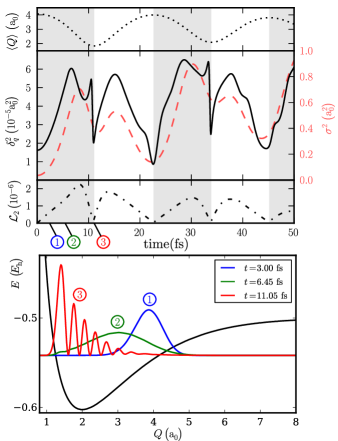
Figure 5: (Color online) Top panel: The expectation value of the internuclear distance $\left\langle Q\right\rangle$ (black dotted line) as a function of time. Second panel: The squared value of the correlation length $\delta_{q}^{2}$ (black solid line) and the squared variance of the internuclear distance $\sigma^{2}=\left\langle Q^{2}\right\rangle-\left\langle Q\right\rangle^{2}$ (red dashed line) as a function of time. Thrid panel: The error of the optimization per grid point, $\mathcal{L}_{2}=\frac{1}{N}\big{\|}\frac{\partial}{\partial t}\rho_{c}+\vec{\nabla}_{e}\cdot\vec{j}_{c}\big{\|}_{2}$, (black dashed dotted line) in units of $E_{\rm h}/(\hbar a_{0}^{3})$ as a function of time. Regions, where the expectation value of the internuclear distance $\left\langle Q\right\rangle$ decreases, are shaded gray. Notice the different scaling. Bottom panel: Nuclear wavepacket at three times during the first half oscillation cycle: $t=3.00\,{\rm fs}$ (blue), $t=6.45\,{\rm fs}$ (green), and $t=11.05\,{\rm fs}$ (red).

The second panel in Fig. 5 depicts the time evolution of the correlation length squared, $\delta_{q}^{2}$, for two complete nuclear oscillation periods. These can be identified from the expectation value of the internuclear distance, shown in the top panel. A clear and unique optimal value of the correlation length is found at each timestep, which can further be seen to be very small and exhibit a smooth periodic behavior. The dashed line in the central panel represents the squared variance of the nuclear wavepacket, $\sigma^{2}$. Between the turning points, both the correlation length and the nuclear wavepacket variance behave similarly. This can be understood in simple physical terms: as the nuclear wavepacket moves towards the bottom of the well, the nuclei acquire a larger velocity and the electrons drag on a longer scale behind the molecular motion. This is captured by the correlation length, which weights the importance of non-adiabatic couplings and momentum transfer between nuclear and electronic degrees of freedom. At the turning points, the correlation length is subject to a more structured time evolution even though the nuclear variance remains smooth.

In order to confirm that the complex structure of $\delta_{q}^{2}$ conveys physical meaning, the residual error from the optimization in Eq. (19), $\mathcal{L}_{2}$, is reported per grid point in the third panel of Fig. 5. This error remains at least one order of magnitude smaller that the main features of the electron flow reported in Fig. 2 and it correlates with the variance of the internuclear distance, $\sigma^{2}$. Moreover, it is smoother and less structured than the time evolution of the correlation length. This can be understood on the basis of the nuclear variance, as a wider spread of the underlying nuclear velocity field will render minimization of Eq. (19) with a single parameter less accurate. Thus, the fast oscillating structures observed in the correlation length at the inner classical turning point - and to a lesser extent at the outer ones - have a physical origin other than the nuclear dynamics.

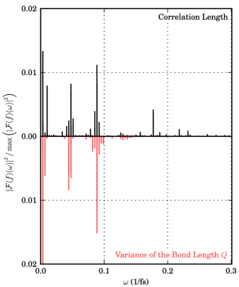
Figure 6: (Color online) Normalized power spectra of the correlation length squared $\delta_{q}^{2}$ (black) and the variance of the internuclear distance $\sigma^{2}=\langle Q^{2}\rangle-\langle Q\rangle^{2}$ (red) as a function of the frequency $\omega$. The dynamics was simulated up to twice the nuclear recurrence time of $T=293.16\,{\rm fs}$ with a time step width of $\Delta t=0.3\,{\rm fs}$.

The comparison of the correlation length and the internuclear distance variance becomes clearer when looking at the power spectrum of their time evolution, as shown in Fig. 6. Both quantities contain several common components at low frequencies, reflecting the classical behavior of the electrons instantaneously reacting to the nuclear motion between the turning points. However, the spectrum of $\delta_{q}^{2}$ is more complex and shows additional peaks at higher frequencies. These are attributed to interference effects in the nuclear wavepacket upon reflection, which can be observed in the bottom panel of Fig. 5, where the nuclear wavepackets at $t=3.00\,{\rm fs}$, $t=6.45\,{\rm fs}$, and $t=11.05\,{\rm fs}$ are depicted. The latter shows strongly oscillatory structures, which explains the rapid variation of the correlation length at the turning points, as the electrons react more substantially to the intricate structure of the nuclear wavepacket. As such, this is a purely quantum mechanical effect stemming from the implicit electron dynamics alone.

V Conclusions

A fundamental problem of the Born-Oppenheimer approximation is that the electronic degrees of freedom are represented using real-valued wavefunctions, leading to the counterintuitive results that electrons remain stationary upon nuclear dynamics instead of flowing along with the molecular motion. In this work, we presented a numerical approach to circumvent this intrinsic problem within the standard framework of the Born-Oppenheimer approximation: the Born-Oppenheimer Broken Symmetry (BOBS) approach to the adiabatic electronic flux density. In a very first step, we introduced a translation operator and applied it to the total (vibronic) density matrix operator. Tracing out the nuclear degrees of freedom, the electronic probability density could be forced to satisfy the electronic continuity equation approximately using a numerical minimization procedure. This cost functional minimization depends on a single control parameter, the correlation length $\delta_{q}$, which we interpret as an electron-nucleus correlation in nuclear configuration space. The electron flow and associated electronic flux density obtained from our Born-Oppenheimer Broken Symmetry procedure are real-valued, as opposed to the AIMD-based ”time-shift“ flux approach of Okayama and Takatsuka.

The application of the translation operator to the electronic wavefunction in the position representation can become computationally prohibitively expensive, and a Taylor series expansion of the correlated electron density to second order was introduced, yielding nearly identical results as the non-linear cost minimization. The series expansion revealed that the physical origin of the electronic flux density observed in the BOBS ansatz is the first-order non-adiabatic coupling between electrons and nuclei, with second order non-adiabatic contributions contributing to the electron flow. Because of its computational efficiency, this approach could be easily applied to very large systems.

A vibrating hydrogen molecular ion ${\rm H}_{2}^{+}$ in the electronic ground state ${}^{2}\Sigma^{+}_{g}$ served as a test system for the BOBS approach. The electron flow was seen to be hardly affected by translation of the density matrix and compared well with the non-Born-Oppenheimer results, while the electronic flux density qualitatively recovered the correct features - symmetry at the inversion center and the turning point, nodal planes perpendicular to the nuclear motion, etc - at all times. Analysis of the time evolution of the correlation length demonstrated that, while a large portion of the implicit electron dynamics can be correlated to the variance of the time-evolving nuclear wavepacket, electrons show a stronger quantum mechanical character at the turning points due to interference effects upon reflection.

Because of its simplicity, the Born-Oppenheimer Broken Symmetry (BOBS) approach to the adiabatic electronic flux density appears as a possibly valuable semi-quantitative tool for understanding the electron dynamics of many other chemical processes. A unique feature of the BOBS method is the explicit consistency enforcement of the electronic continuity equation at all times, which simultaneously provides an error estimate. In order to improve the quantitative predictive power of the method, handling the different components of the electronic flux density with separate values for the correlation length $\delta_{q}\to\{\delta_{q_{x}},\delta_{q_{y}},\delta_{q_{z}}\}$, could be used to reduce the undesirable localized behavior.

Appendix A Vibrational eigenstates representation

For a given initial condition, the nuclear wavepacket $\chi$ can be expanded in the eigenstates basis of the associated nuclear Hamiltonian $H_{\rm nuc}\chi_{n}=E_{n}\chi_{n}$ to

$$\chi =\sum_{n}a_{n}e^{-\imath E_{n}t/\hbar}\chi_{n}.$$ (23)

Accordingly, the derivatives of the nuclear wavepacket are defined as

$$\frac{\partial}{\partial t}\chi =-\frac{\imath}{\hbar}\sum_{n}a_{n}E_{n}e^{-\imath E_{n}t/\hbar}\chi_{n}$$ (24)

$$\chi^{\prime} =\nabla_{Q}\chi=\sum_{n}a_{n}e^{-\imath E_{n}t/\hbar}\chi_{n}^{\prime}.$$

Inserting this basis set representation in the correlated continuity equation Eqs. (18-16) yields

$$\frac{\partial}{\partial t} \rho_{c}=-\int{\rm d}Q\left(\varphi^{-\delta_{q}}\varphi^{+\delta_{q}}\right)$$ (25)

$$\times\sum_{m<n}\omega_{mn}a_{n}a_{m}\left(\chi_{n}^{-\delta_{q}}\chi_{m}^{+\delta_{q}}+\chi_{n}^{+\delta_{q}}\chi_{m}^{-\delta_{q}}\right)\sin\left(\omega_{mn}t\right)$$

and

$$-\vec{\nabla}_{e}\cdot \vec{j}_{c}=-\frac{\hbar}{m_{e}}\vec{\nabla}_{e}\cdot\int{\rm d}Q\left(\varphi^{+\delta_{q}}\vec{\nabla}_{e}\varphi^{-\delta_{q}}-\varphi^{-\delta_{q}}\vec{\nabla}_{e}\varphi^{+\delta_{q}}\right)$$ (26)

$$\times\sum_{m<n}a_{n}a_{m}\left(\chi_{n}^{-\delta_{q}}\chi_{m}^{+\delta_{q}}-\chi_{n}^{+\delta_{q}}\chi_{m}^{-\delta_{q}}\right)\sin\left(\omega_{mn}t\right)$$

with $\omega_{mn}=\frac{E_{m}-E_{n}}{\hbar}$ and $a_{n}\in\Re$. Eqs. (25, 26) can be trivially extended to complex-valued expansion coefficients $a_{n}$. Note that the left [cf. Eq. (25)] and the right-hand-side [cf. Eq. (26)] of the correlated continuity equation in the basis set representation oscillate with the same sinusoidal behavior. After some manipulations, the Taylor series expansion Eqs. (LABEL:taylor_jc_left, 22) thus yields

$$\frac{\partial}{\partial t}\rho_{c} = -2\int{\rm d}Q\left(\left|\varphi\right|^{2}+\delta_{q}^{2}\left(\varphi^{\prime\prime}\varphi-\varphi^{\prime}\varphi^{\prime}\right)\right)\sum_{m<n}\omega_{mn}a_{n}a_{m}\chi_{n}\chi_{m}\sin\left(\omega_{mn}t\right)$$ (27)

$$-\delta_{q}^{2}\int{\rm d}Q\left|\varphi\right|^{2}\sum_{m<n}\omega_{mn}a_{n}a_{m}\left(\chi_{n}^{\prime\prime}\chi_{m}-2\chi_{n}^{\prime}\chi_{m}^{\prime}+\chi_{n}\chi_{m}^{\prime\prime}\right)\sin\left(\omega_{mn}t\right)+O\left(\delta_{q}^{4}\right)$$

$$-\vec{\nabla}_{e}\cdot\vec{j}_{c} = +\frac{2\hbar\delta_{q}^{2}}{m_{e}}\vec{\nabla}_{e}\cdot\int{\rm d}Q\left(\varphi\vec{\nabla}_{e}\varphi^{\prime}-\varphi^{\prime}\vec{\nabla}_{e}\varphi\right)\sum_{m<n}a_{n}a_{m}\left(\chi_{n}\chi_{m}^{\prime}-\chi_{n}^{\prime}\chi_{m}\right)\sin\left(\omega_{mn}t\right)+O\left(\delta_{q}^{4}\right).$$ (28)

References

- Born and Oppenheimer (1927) M. Born and R. Oppenheimer, Ann. Physik 20, 30 (1927).
- Eyring (1935) H. Eyring, J. Chem. Phys. 3, 107 (1935).
- Evans and Polanyi (1935) M. G. Evans and M. Polanyi, Trans. Faraday Soc. 31, 875 (1935).
- Polanyi (1987) J. C. Polanyi, Science 236, 680 (1987).
- Mita (2001) K. Mita, Am. J. Phys. 69, 470 (2001).
- Dixit et al. (2012) G. Dixit, O. Vendrell, and R. Santra, PNAS 109, 11636 (2012).
- Dixit et al. (2013) G. Dixit, J. M. Slowik, and R. Santra, Phys. Rev. Lett. 110, 137403 (2013).
- Suominen and Kirrander (2014) H. J. Suominen and A. Kirrander, Phys. Rev. Lett. 112, 043002 (2014).
- Frohnmeyer and Baumert (2000) T. Frohnmeyer and T. Baumert, Appl. Phys. B 71, 259 (2000).
- Ergler et al. (2006) T. Ergler, A. Rudenko, B. Feuerstein, K. Zrost, C. D. Schröter, R. Moshammer, and J. Ullrich, Phys. Rev. Lett. 97, 193001 (2006).
- Manz et al. (2013) J. Manz, J. F. Pérez-Torres, and Y. Yang, Phys. Rev. Lett. 111, 153004 (2013).
- Fonseca Guerra et al. (2004) C. Fonseca Guerra, J.-W. Handgraaf, E. J. Baerends, and F. M. Bickelhaupt, J. Comput. Chem. 25, 189 (2004).
- Schrödinger (1926) E. Schrödinger, Ann. Physik 81, 109 (1926).
- Born and Huang (1954) M. Born and K. Huang, Dynamical Theory of Crystal Lattices. (Oxford University Press, Oxford, 1954).
- Paramonov (2005) G. K. Paramonov, Chem. Phys. Lett. 411, 350 (2005).
- Kono et al. (2006) H. Kono, Y. Sato, M. Kanno, K. Nakai, and T. Kato, Bull. Chem. Soc. Jpn. 79, 196 (2006).
- Karr and Hilico (2006) J. P. Karr and L. Hilico, J. Phys. B 39, 2095 (2006).
- Niederhausen et al. (2012) T. Niederhausen, U. Thumm, and F. Martí n, J. Phys. B 45, 105602 (2012).
- Ishikawa et al. (2012) A. Ishikawa, H. Nakashima, and H. Nakatsuji, Chem. Phys. 401, 62 (2012).
- Pérez-Torres (2013) J. F. Pérez-Torres, Phys. Rev. A 87, 062512 (2013).
- Bubin et al. (2009) S. Bubin, F. Leonarski, M. Stanke, and L. Adamowicz, Chem. Phys. Lett. 477, 12 (2009).
- Chen and Anderson (1995) B. Chen and J. B. Anderson, J. Chem. Phys. 102, 2802 (1995).
- Mátyus et al. (2011) E. Mátyus, J. Hutter, U. Müller-Herold, and M. Reiher, J. Chem. Phys. 135, 204302 (2011).
- Mátyus and Reiher (2012) E. Mátyus and M. Reiher, J. Chem. Phys. 137, 024104 (2012).
- D. J. Diestler (2012) D. J. Diestler, J. Phys. Chem. A 116, 2728 (2012).
- Diestler et al. (2012) D. J. Diestler, A. Kenfack, J. Manz, and B. Paulus, J. Phys. Chem. A 116, 2736 (2012).
- Diestler et al. (2013) D. J. Diestler, A. Kenfack, J. Manz, B. Paulus, J. F. Pérez-Torres, and V. Pohl, J. Phys. Chem. A (2013).
- Hermann et al. (2014) G. Hermann, B. Paulus, J. F. Pérez-Torres, and V. Pohl, Phys. Rev. A 89, 052504 (2014).
- Okuyama and Takatsuka (2009) M. Okuyama and K. Takatsuka, Chem. Phys. Lett. 476, 109 (2009).
- Bredtmann et al. (2015) T. Bredtmann, D. J. Diestler, S.-D. Li, J. Manz, J. F. Pérez-Torres, W.-J. Tian, Y.-B. Wu, Y. Yang, and H.-J. Zhai, Phys. Chem. Chem. Phys. 17, 29421 (2015).
- Nafie (1983) L. A. Nafie, J. Chem. Phys. 79, 4950 (1983).
- Patchkovskii (2012) S. Patchkovskii, J. Chem. Phys. 137, 084109 (2012).
- Diestler (2013) D. J. Diestler, J. Phys. Chem. A 117, 4698 (2013).
- Runge and Gross (1984) E. Runge and E. K. U. Gross, Phys. Rev. Lett. 52, 997 (1984).
- Werner et al. (2012) H.-J. Werner, P. J. Knowles, G. Knizia, F. R. Manby, M. Schütz, et al., “Molpro, version 2012.1, a package of ab initio programs,” (2012), see http://www.molpro.net.
- Dunning (1989) T. H. Dunning, J. Chem. Phys. 90, 1007 (1989).
- Hermann et al. (2015) G. Hermann, V. Pohl, and A. Schild, “orbkit: A toolbox for post-processing quantum chemical wavefunction data,” (2015), see http://sourceforge.net/p/orbkit.
- Schmidt and Lorenz (2013) B. Schmidt and U. Lorenz, “Wavepacket 4.9: A matlab program package for quantum-mechanical wavepacket propagation and time-dependent spectroscopy,” (2013), see http://wavepacket.sourceforge.net.
- Jones et al. (001 ) E. Jones, T. Oliphant, P. Peterson, et al., “SciPy: Open source scientific tools for Python,” (2001-), see http://www.scipy.org/.