UWThPh-2015-28

Harold C. Steinacker

Faculty of Physics, University of Vienna
Boltzmanngasse 5, A-1090 Vienna, Austria

Abstract

We describe a stabilization mechanism for fuzzy $S^{4}_{N}$ in the Euclidean IIB matrix model due to vacuum energy in the presence of a positive mass term. The one-loop effective potential for the radius contains an attractive contribution attributed to supergravity, while the mass term induces a repulsive contribution for small radius due to SUSY breaking. This leads to a stabilization of the radius. The mechanism should be pertinent to recent results on the genesis of 3+1-dimensional space-time in the Minkowskian IIB model.

1 Introduction

It is widely expected that space-time should have some kind of quantum structure at short distances. On the other hand, we known that (local) Lorentz invariance is respected to a very high precision. Reconciling these two requirements is a non-trivial task. In two dimensions, the fuzzy sphere $S^{2}_{N}$ [1, 2] or fuzzy (anti-) de Sitter space $(A)dS^{2}_{N}$ [3, 4] provide examples of quantum geometries which are compatible with the full isometry group $SO(3)$ and $SO(2,1)$, respectively. This is possible because the underlying Poisson structures are invariant. However in 4 dimensions, any Poisson structure will necessarily break the local isometry group; in fact, $S^{4}$ does not even admit any symplectic structure at all.

Nevertheless, there is a four-dimensional version of the fuzzy sphere $S^{4}_{N}$ [5, 6] which is fully covariant under $SO(5)$, and has a finite number of “quantum cells”. The price to pay is a tower of higher spin modes [7], which arise because $S^{4}_{N}$ has internal structure and is more properly described as a $S^{2}_{N+1}$ bundle over $S^{4}$ [8, 9, 10, 11, 12], or as a twisted stack of $N+1$ four-spheres. Nevertheless $S^{4}_{N}$ can be realized in matrix models, and one may hope that these higher-spin modes acquire a mass via quantum effects in that setting. If that turns out to be true, this type of background may allow to reconcile the ideas of emergent gravity in matrix models [13, 14] with Lorentz invariance. It has indeed been argued on different grounds that gravity should emerge on a Lorentzian analog of this space [15].

In the present paper, we consider the realization of fuzzy $S^{4}_{N}$ within the IIB or IKKT matrix model [16], taking into account quantum corrections. This is motivated in part by the remarkable recent results of computer-simulation of the Lorentzian IIB model. It was found [17] that a 3+1-dimensional extended geometry arises dynamically in this model, interpreted as emergent cosmological space-time. To define the Lorentzian model, an IR regularization of the model is required. Such a regularization can be viewed as analytic continuation of a bosonic mass term. This suggests that to understand these findings and the relation with the Euclidean case, an analogous mass term should also be introduced in the Euclidean IIB model.

The main result of the present paper is that introducing a positive mass term in the Euclidean IIB model leads indeed to an interesting stabilization mechanism for fuzzy geometries at one loop, which in particular stabilizes the radius of $S^{4}_{N}$. This is quite remarkable and perhaps surprising: at the classical level $S^{4}_{N}$ is certainly not a solution, since the radius is not stabilized. It would formally be a solution for a negative mass term, but then the model becomes unstable, so this is not an option. One might try to stabilize it by adding a “flux” term of order 5 to the model [9], however this spoils the good UV properties of the model, and stabilization is lost at the quantum level [18].

Remarkably, adding a positive mass term to the supersymmetric IIB model does provide a stabilization mechanism at one-loop: Without mass term, the residual (finite) one-loop effects lead to an attractive (negative) contribution to the effective potential, which may be interpreted in terms of supergravity [16, 19]. However this effect is independent of the radius, and does not stabilize $S^{4}_{N}$ in the IIB model. Upon adding a (small) positive mass term, the bosonic quantum fluctuations are suppressed over the fermionic fluctuations, so that the latter lead to a positive contribution to the effective potential. This effect is large for small radius $r$ of $S^{4}_{N}$ as the SUSY breaking is significant, but it is small for large $r$ since then the SUSY breaking is insignificant, and the attractive contribution attributed to supergravity prevails. As a result, the effective potential has a stable minimum as a function of $r$, thus stabilizing $S^{4}_{N}$. We elaborate this effect in section 4 by performing a detailed one-loop computation, integrating out all fluctuation modes except for the lowest (would-be) massless modes. The result is argued to be robust for large $N$, and it only applies to the maximally supersymmetric IIB model.

The mechanism under consideration is not restricted to the particular $S^{4}_{N}$ background. However, it is very plausible that the $S^{4}_{N}$ should be preferred dynamically over less symmetric spaces such as $T^{2}\times T^{2}$ [20] or $S^{2}\times S^{2}$ or ${\mathbb{C}}P^{2}$. Moreover, the stabilization mechanism does not apply to branes with dimension 6 or higher. We also find in section 4.2 that for suitable parameters, fuzzy $S^{4}_{N}$ has lower energy than a fuzzy two-sphere. On the other hand, we also find a preference towards high-rank gauge groups i.e. stacks of multiple branes. Thus we certainly cannot draw any non-perturbative conclusions. Nevertheless, the observed stabilization of $S^{4}_{N}$ at one loop indicates that this semi-classical geometry may be a good step towards unraveling the structure of space-time.

2 Fuzzy $S^{4}_{N}$

Let $\gamma_{i},\ i=1,...,5$ be the gamma matrices associated to $SO(5)$, which act on ${\mathbb{C}}^{4}$. Fuzzy $S^{4}_{N}$ [5, 6] is defined in terms of the following “many-particle” version of $\gamma_{i}$

$$X_{i} =\frac{1}{2}\big{(}\gamma_{i}\otimes 1\otimes...\otimes 1+...+1\otimes...\otimes 1\otimes\gamma_{i}\Big{)},\qquad i=1,2,...,5$$ (2.1)

acting on

$${\cal H}_{N}=\big{(}{\mathbb{C}}^{4}\otimes...\otimes{\mathbb{C}}^{4}\big{)}_{\rm sym}=(0,N)_{SO(5)}\ .$$ (2.2)

We denote irreducible highest weight representation by the Dynkin indices. This can be written succinctly as

$$X_{i}=\frac{1}{2}a^{\dagger}_{\alpha}(\gamma_{i})^{\alpha}_{\ \beta}a^{\beta}$$ (2.3)

with 4 bosonic oscillators

$$[a^{\beta},a^{\dagger}_{\alpha}]=\delta_{\alpha}^{\beta}$$ (2.4)

acting on the Fock space ${\cal H}_{N}=a^{\dagger}_{i_{1}}...a^{\dagger}_{i_{N}}|0\rangle$. Their commutation relations are obtained as

$$[X_{i},X_{j}] =:i\,{\cal M}_{ij}$$ (2.5)

$$[{\cal M}_{ij},{\cal M}_{kl}] =i(\delta_{ik}{\cal M}_{jl}-\delta_{il}{\cal M}_{jk}-\delta_{jk}{\cal M}_{il}+\delta_{jl}{\cal M}_{ik})$$ (2.6)

$$[{\cal M}_{ij},X_{k}] =i(\delta_{ik}X_{j}-\delta_{jk}X_{i}).$$ (2.7)

In particular,

$${\cal M}_{ij}=a^{\dagger}M_{ij}a,\qquad M_{ij}=\frac{1}{4i}[\gamma_{i},\gamma_{j}]$$ (2.8)

generate the $SO(5)$ rotations on the algebra $End({\cal H}_{N})$ generated by the $X_{i}$. This means that fuzzy $S^{4}_{N}$ is a Snyder-type noncommutative space [21], where ${\cal M}_{ij}$ generate the $SO(5)$ transformations of the $X_{i}$, which transform in the $(1,0)$ of $SO(5)$.

Now consider the $SO(5)$-invariant operator $\sum_{i}X_{i}^{2}$. Since $(0,N)$ is irreducible, it must be $\sim\mbox{1 \kern-5.89996pt{\rm l}}$, and the constant is easily found to be [6]

$$\hat{R}^{2}:=\sum_{i}X_{i}^{2}=\frac{1}{4}N(N+4)\mbox{1 \kern-5.89996pt{\rm l}}=:r_{N}^{2}\mbox{1 \kern-5.89996pt{\rm l}}\ .$$ (2.9)

Together with the $SO(5)$ covariance, this strongly suggests an interpretation in terms of $S^{4}$ with radius $r_{N}=\frac{1}{2}\sqrt{N(N+4)}$. Indeed the above construction is entirely analogous to that of the fuzzy sphere [1], using $SO(5)$ instead of $SO(3)$.

To gain some intuition, consider the north pole $p\in S^{4}$, which is invariant under the local stabilizer group $SO(4)\subset SO(5)$. We can then decompose the ${\cal M}_{ij}$ into rotation generators

$${\cal M}_{\mu\nu},\qquad\mu,\nu\in\{1,2,3,4\}$$ (2.10)

which generate the “local” $SO(4)$, and

$$P_{\mu} =\frac{1}{r_{N}}{\cal M}_{\mu 5}\ \ ,\qquad\mu\in\{1,2,3,4\}$$ (2.11)

which correspond to “translations” moving $p$ along $S^{4}$; the latter transform as vectors of $SO(4)\cong SU(2)_{L}\times SU(2)_{R}$. In particular, (2.7) implies

$$[P_{\mu},X_{\nu}]=i\delta_{\mu\nu}\frac{1}{r_{N}}X_{5}$$ (2.12)

which reduces to the canonical commutation relations upon replacing $X^{5}\to r_{N}$ at or near $p$, and (2.6) implies

$$[P_{\mu},P_{\nu}] =-i\frac{1}{r_{N}^{2}}{\cal M}_{\mu\nu}\ .$$ (2.13)

Thus the Poincare group is recovered as usual from $SO(5)$ via an Inönü-Wigner contraction.

Fuzzy $S^{4}_{N}$ versus fuzzy ${\mathbb{C}}P^{3}_{N}$.

Although the above results seem very straightforward, it turns out that fuzzy $S^{4}_{N}$ is more properly understood as a degenerate “projection” of fuzzy ${\mathbb{C}}P^{3}_{N}$ [10, 22, 11, 12, 23, 24]. This can be seen simply by extending (2.3) to the full set of $\mathfrak{su}(4)\cong\mathfrak{so}(6)\supset\mathfrak{so}(5)$ generators

$$X_{A}=a^{\dagger}_{\alpha}(M_{A})^{\alpha}_{\ \beta}a^{\beta}$$ (2.14)

acting on

$${\cal H}_{N}=(0,N)_{SO(5)}=(0,0,N)_{SU(4)}$$ (2.15)

where $M_{A}$ are the $\mathfrak{su}(4)$ generators acting on ${\mathbb{C}}^{4}$. Organizing $A=(a,b)_{a<b\leq 6}$ as a basis of $\mathfrak{so}(6)$ and identifying

$$\gamma_{i}=2M_{i6}\ ,$$ (2.16)

we recover the previous generators $X_{i}$ (2.3) from this extended set of generators. Moreover, since ${\cal H}_{N}=(0,N)$ of $SO(5)$ is equivalent to $(0,0,N)$ of $SU(4)$, (2.14) can be rewritten as

$$X_{A}=\pi_{N}(M_{A})$$ (2.17)

acting on ${\cal H}_{N}$. This is precisely the construction of fuzzy ${\mathbb{C}}P^{3}_{N}$ [25, 26], which is a quantization of ${\mathbb{C}}P^{3}$ viewed as coadjoint orbit in $\mathfrak{su}(4)\cong{\mathbb{R}}^{15}$ with Poisson structure $\{X_{A},X_{B}\}=f_{AB}^{C}X_{C}$ corresponding to the Kirillov-Kostant symplectic form, with commutation relations

$$[X_{A},X_{B}]=if_{AB}^{C}X_{C}\ .$$ (2.18)

In particular, we recognize the ${\cal M}_{ij}$ (2.5) as generators of $\mathfrak{so}(5)\subset\mathfrak{so}(6)=\mathfrak{su}(4)$ acting on ${\cal H}_{N}$. More importantly, the original $X_{i},\ i=1,...,5$ are now recognized as a subset of the 15 quantized embedding functions

$$X_{A}\sim x_{A}:\quad{\mathbb{C}}P^{3}\hookrightarrow\mathfrak{su}(4)\cong{\mathbb{R}}^{15}$$ (2.19)

of the 6-dimensional coadjoint orbit ${\mathbb{C}}P^{3}$ in ${\mathbb{R}}^{15}$. Here $\sim$ indicates the semi-classical limit. Dropping the extra generators amounts to a projection ${\mathbb{C}}P^{3}\subset{\mathbb{R}}^{15}\to S^{4}\subset{\mathbb{R}}^{5}$. This corresponds to the Hopf map ${\mathbb{C}}P^{3}\to S^{4}$ along a $S^{2}$ fiber, as discussed in appendix A.

The bottom line is that fuzzy $S^{4}_{N}$ is not the quantization of $S^{4}$ with some Poisson structure, but it is a 4-dimensional degenerate embedding of fuzzy ${\mathbb{C}}P^{3}_{N}$ with squashed $S^{2}_{N+1}$ fiber. The “local noncommutativity” ${\cal M}_{\mu\nu}$ can then be understood as a fibration with self-dual 2-forms on $S^{4}$ which vary along the $S^{2}$ fiber, as explained in more detail below. This allows to preserve full covariance under $SO(5)$, and explains its somewhat complicated algebraic structure including apparent non-associativity [7, 8] and higher-spin fields.

Useful results on the fuzzy $S^{4}$ algebra.

We collect some more results for fuzzy $S^{4}_{N}$. From (2.7) one obtains immediately

$$\Box_{X}X_{i}\equiv[X_{j},[X_{j},X_{i}]]=\,4\,X_{i}\ .$$ (2.20)

We also note the identity

$${\cal M}_{ij}X_{j}+X_{j}{\cal M}_{ij}=[X_{i},r_{N}^{2}]=0$$ (2.21)

which states that the ${\cal M}_{ij}$ are tangential. Now consider the following Casimir operator

$$\epsilon^{ijklm}X_{i}X_{j}X_{k}X_{l}X_{m}=-\frac{1}{4}{\cal M}_{ij}{\cal M}_{kl}X_{m}\epsilon^{ijklm}=C^{5}\mbox{1 \kern-5.89996pt{\rm l}}\ .$$ (2.22)

To evaluate this, we recall $X_{m}={\cal M}_{m6}$ (2.16), so that

$${\cal M}_{ij}{\cal M}_{kl}X_{m}\epsilon^{ijklm} =\frac{1}{6}{\cal M}_{ij}{\cal M}_{kl}{\cal M}_{mn}\epsilon^{ijklmn}\ .$$ (2.23)

This is a totally symmetric cubic invariant of $\mathfrak{su}(4)$ which can only be the $d^{ABC}{\cal M}_{A}{\cal M}_{B}{\cal M}_{C}$ tensor, which for ${\mathbb{C}}P^{3}_{N}$ is given by [25, 26]

$$d{\cal M}{\cal M}{\cal M}=\frac{3}{16}(N+2)N(N+4)\ .$$ (2.24)

Therefore $C^{5}=c(N+2)r_{N}^{2}$ where $c$ is a constant independent of $N$. This is found to be $c=\frac{1}{4}$ for $N=1$, and it follows that

$$\epsilon^{ijklm}X_{i}X_{j}X_{k}X_{l}X_{m} =(N+2)r_{N}^{2}$$ (2.25)

consistent with [6, 9].

2.1 Alternative interpretation: stack of $N+1$ branes

We have just explained the interpretation of fuzzy $S^{4}_{N}$ as “squashed” fuzzy ${\mathbb{C}}P^{3}_{N}$ with degenerate fiber $S^{2}_{N+1}$. There is an alternative interpretation as a twisted stack of $N+1$ spherical branes (cf. [6, 8, 28]), carrying a $\mathfrak{u}(N+1)$-valued noncommutative Yang-Mills gauge field with flux ${\cal M}^{\mu\nu}$. This gauge field configuration is necessarily non-trivial, since $S^{4}$ does not admit any symplectic form due to $H^{2}(S^{4})=0$. As explained in appendix A, the generators ${\cal M}^{\mu\nu}$ of the local $\mathfrak{so}(4)=\mathfrak{su}(2)_{L}\times\mathfrak{su}(2)_{R}$ act on the local $S^{2}$ fiber only via $\mathfrak{su}(2)_{L}$, while $\mathfrak{su}(2)_{R}$ acts trivially. These $\mathfrak{su}(2)_{L}$ generators $J_{k}^{(L)}$ generate the local $S^{2}_{N+1}$. This means that ${\cal M}^{\mu\nu}$ is a self-dual $\mathfrak{u}(N+1)$ “instanton” configuration

$${\cal M}^{\mu\nu} =\epsilon^{\mu\nu k}_{L}\,J_{k}^{(L)}\ .$$ (2.26)

Another way to see this is via coherent states [28]. As usual, such a $\mathfrak{u}(N+1)$-valued flux can be interpreted as a gauge field on a stack of $N+1$ noncommutative branes, which are identified e.g. by diagonalizing $J_{3}^{(L)}$, or by choosing $N+1$ coherent states $|i\rangle$ on $S^{2}_{N}$. Then the modes $|i\rangle\langle j|\in\mathfrak{u}(N+1)$ can be interpreted as “string” connecting two such sheets, and we can assign a Poisson structure

$$\langle i|{\cal M}^{\mu\nu}|i\rangle \sim\theta^{\mu\nu}=\{x^{\mu},x^{\nu}\}$$ (2.27)

to these $N+1$ leaves covering $p\in S^{4}$.

We can provide a non-trivial consistency check of this semi-classical picture. To this end, we evaluate (2.25) at the north pole (or via $\langle i|.|i\rangle$) in terms of the Pfaffian

$${\rm Pf}\theta^{\mu\nu}=\frac{1}{2}\epsilon_{\mu\nu\rho\sigma}\theta^{\mu\nu}\theta^{\rho\sigma}$$ (2.28)

which gives

$$(N+2)r_{N}^{2}=\epsilon^{ijkl5}X_{i}X_{j}X_{k}X_{l}X_{5}\sim r_{N}\epsilon_{\mu\nu\rho\sigma}\theta^{\mu\nu}\theta^{\rho\sigma}=2r_{N}\,{\rm Pf}\theta^{\mu\nu}\ .$$ (2.29)

Thus

$${\rm Pf}\theta^{\mu\nu}\ \sim\ r_{N}^{2}$$ (2.30)

for large $N$. Now the semi-classical formula $tr\sim\frac{1}{(2\pi)^{2}}\int\frac{1}{2}\omega^{2}$ for 4-dimensional symplectic spaces applied to the $N+1$ (twisted) leaves gives

$$\frac{8}{3}r_{N}^{6} \sim trXXXXX\epsilon\sim\frac{N+1}{(2\pi)^{2}}\int\frac{1}{2}\omega^{2}2r_{N}\,{\rm Pf}\theta^{\mu\nu}$$

$$=2r_{N}(N+1)\frac{1}{(2\pi)^{2}}Vol(S^{4})=\frac{4}{3}r_{N}^{5}(N+1)$$ (2.31)

noting that the Pfaffian and $\frac{1}{2}\omega^{2}$ cancel each other, giving $\int\frac{1}{2}\omega^{2}{\rm Pf}\theta^{\mu\nu}=Vol(S^{4})=\frac{8\pi^{2}}{3}r_{N}^{4}$. This is consistent with $r_{N}\sim\frac{N}{2}$ (2.9) for large $N$, confirming the above semi-classical picture. In other words, fuzzy $S^{4}_{N}$ has approximately $\dim{\cal H}_{N}\sim\frac{1}{6}N^{3}$ “noncommutative” volume quanta $L_{NC}^{4}$ distributed over $(N+1)$ times the metric volume of $S^{4}$,

$$\frac{1}{6}N^{3}L_{NC}^{4} \sim(N+1)\frac{8\pi^{2}}{3}r_{N}^{4}\sim\frac{\pi^{2}}{6}N^{5}\ .$$ (2.32)

Hence the scale of noncommutativity i.e. the effective uncertainty scale is set by

$$L_{NC} \sim\sqrt{N\pi}\ .$$ (2.33)

On the other hand, each volume $L_{NC}^{4}$ in target space is covered by $(N+1)$ such cells, which reflects the internal structure of $S^{4}_{N}$. Thus one might also argue that the “atoms” of space have the size

$$L_{0}^{4} =\frac{16\pi^{2}}{N^{4}}r_{N}^{4},\qquad L_{0}\sim\sqrt{\pi}$$ (2.34)

which is of order one. The physical significance of these two scales and their possible relation to the Planck scale remains to be elucidated.

2.2 Functions and harmonics on fuzzy $S^{4}$

The algebra of functions $End({\cal H}_{N})$ decomposes into the $SU(4)$ harmonics

$$End({\cal H}_{N}) =(0,0,N)\otimes(N,0,0)=\bigoplus\limits_{n=0}^{N}(n,0,n)$$ (2.35)

which is a truncation of the classical algebra of (polynomial) functions on ${\mathbb{C}}P^{3}$,

$$Pol({\mathbb{C}}P^{3})=\bigoplus\limits_{n=0}^{\infty}(n,0,n)\ .$$ (2.36)

Each of these $(n,0,n)$ decompose into the $SO(5)$ harmonics as follows

$$(n,0,n)=\bigoplus\limits_{m=0}^{n}(n-m,2m)\ .$$ (2.37)

The $(n,0)$ modes correspond to the (totally symmetrized traceless) polynomial functions $P_{n}(X_{i})$ on $S^{4}$ of degree $n$. The $(n-m,2m)$ modes with $m\neq 0$ have a non-trivial dependence along the $S^{2}$ fiber, i.e. they transform non-trivially under the local stabilizer group $SU(2)_{L}\times SU(2)_{R}$ at fixed $p\in S^{4}$, hence they correspond to higher spin modes. Thus all “bosonic” higher spin modes of $SO(5)$ arise precisely once in $End({\cal H}_{N})$, while the fermionic $(n,k)$ modes with odd $k$ modes will be recovered in section 3.3.

We would like to have a more explicit description of these modes. To this end, we denote the highest weight vector in $(1,0)$ by $X_{1}^{+}$, and observe that the $X_{5}$ generator is stabilized by $SO(4)\subset SO(5)$ and corresponds to the weight 0 vector in $(1,0)$. Thus the highest weight vector in $(n,0)$ is given by $(X_{1}^{+})^{n}$. Clearly this is also the highest weight vector in $(n,0,n)$, so that all modes in (2.37) are obtained by acting with the universal enveloping algebra ${\cal U}(\mathfrak{su}(4))$ on $(X_{1}^{+})^{n}$.

Now denote with ${\cal M}_{L}^{+}$ the highest weight element in $(0,2)\subset(1,0,1)$; this is the raising operator of $SU(2)_{L}\subset SO(4)$. Clearly ${\cal M}_{L}^{+}$ is obtained by acting with some $SU(4)$ generator $[X_{2}^{+},.]$ (say) on $X_{1}^{+}$. Similarly, acting with $[X_{2}^{+},.]$ on $(X_{1}^{+})^{n}\in(n,0,n)$ gives $(X_{1}^{+})^{n-1}{\cal M}_{L}^{+}$, which is the highest weight vector of $(n-1,2)$. More generally, acting with suitable elements in ${\cal U}(\mathfrak{su}(4))$ on $(X_{1}^{+})^{n}$ generates all the $(X_{1}^{+})^{n-m}({\cal M}_{L}^{+})^{m}$, which are the highest weight vectors in $(n-m,2m)$. Thus we have obtained an explicit description of these higher spin modes:

$$(n-m,2m)={\rm span}\{P_{n-m}(X^{i})P_{m}({\cal M}^{ij})\}\ .$$ (2.38)

We can decompose these modes further w.r.t. the “local” $SO(4)$ structure e.g. at the north pole $p\in S^{4}$, where ${\cal M}_{ij}$ decomposes into the ${\cal M}_{\mu\nu}$ and the $P_{\mu}$ generators. Then e.g. the $(n,2)$ modes on $S^{4}$ comprise modes of the form $f(X)P_{\mu}$ and modes of the form $f(X){\cal M}_{\mu\nu}$. Similarly the $(n,4)$ modes comprise e.g. $f(X)P^{\mu}P^{\nu}$ fields, etc.

Integration over the fiber.

The decomposition (2.37) in particular provides a map which maps any function on ${\mathbb{C}}P^{3}_{N}$ to a spin 0 function on $S^{4}_{N}$, defined by

$$\langle.\rangle:\quad End({\cal H}_{k}) \to End({\cal H}_{k})$$ (2.39)

$$(n,m) \mapsto(n,0)\ .$$ (2.40)

Classically, this amounts to integrating over the local fiber $S^{2}$. Using this projection, the space $\oplus(n,0)$ becomes a commutative but non-associative algebra, which for $N\to\infty$ becomes the classical algebra of functions on $S^{4}$. This algebra is discussed in detail in [7].

2.3 Matrix Laplacian and quadratic Casimirs.

The eigenvalues of the matrix Laplacian

$$f\to\Box f=[X_{i},[X_{i},f]]$$ (2.41)

can be obtained as follows: recalling the identification $X_{i}={\cal M}_{i6}$ and $[X_{i},.]={\cal M}_{i6}^{(ad)}$ on $End({\cal H}_{N})$, we have

$$\Box=[X_{i},[X_{i},.]]=\sum_{i}{\cal M}_{i6}^{(ad)}{\cal M}_{i6}^{(ad)}=C^{2}[\mathfrak{so}(6)]^{(ad)}-C^{2}[\mathfrak{so}(5)]^{(ad)}$$ (2.42)

in terms of the quadratic Casimirs

$$C^{2}[\mathfrak{so}(6)] =\sum_{a<b\leq 6}{\cal M}_{ab}{\cal M}_{ab},$$

$$C^{2}[\mathfrak{so}(5)] =\sum_{a<b\leq 5}{\cal M}_{ab}{\cal M}_{ab}.$$ (2.43)

Their eigenvalues are obtained from $C^{2}=\langle\Lambda,\Lambda+2\rho\rangle=n_{i}\langle\Lambda_{i},\Lambda_{j}\rangle(n_{j}+2)_{j}$ where $\rho=\sum_{i}\Lambda_{i}$ is the Weyl vector, and $n_{i}$ are the Dynkin labels $\Lambda=\sum n_{i}\Lambda_{i}$. This gives

$$C^{2}[\mathfrak{su}(4)](n,0,n) =\frac{1}{4}(n,0,n)\begin{pmatrix}3&2&1\\ 2&4&2\\ 1&2&3\end{pmatrix}\begin{pmatrix}n+2\\ 2\\ n+2\end{pmatrix}=2n(n+3)$$ (2.44)

$$C^{2}[\mathfrak{so}(5)](n-m,2m) =\frac{1}{2}(n-m,2m)\begin{pmatrix}2&1\\ 1&1\end{pmatrix}\begin{pmatrix}n-m+2\\ 2m+2\end{pmatrix}=n(n+3)+m(m+1)$$ (2.45)

in agreement with [10]. Therefore

$$\Box(n-m,2m)=n(n+3)-m(m+1),\qquad m\leq n\ ,$$ (2.46)

which is positive definite as it must be. However, note that $\Box$ is rather small for the $(0,2m)$ modes corresponding to $n=m$. As a check, we recover $\Box X^{i}=4X^{i}$ (2.20). Finally, we can recover (2.9) from (2.43),

$$\sum_{i}X_{i}^{2}=C^{2}[su(4)](0,0,N)-C^{2}[so(5)](0,N)=\frac{1}{4}N(N+4)\ .$$ (2.47)

3 Fluctuations

3.1 Matrix model and mode expansion

We would like to find the fluctuation modes which arise on a $S^{4}_{N}$ background in the Yang-Mills matrix model action with a mass term,

$$S[X] =\frac{1}{g^{2}}\mbox{Tr}\Big{(}-[X_{a},X_{b}][X^{a},X^{b}]\,+\mu^{2}X^{a}X_{a}\Big{)}\ .$$ (3.1)

The equations of motion are

$$(\Box+\frac{1}{2}\mu^{2})X_{a}=0,$$ (3.2)

and (2.20) implies that $S^{4}_{N}$ is a solution for $\mu^{2}=-8$. However such a negative mass term implies an instability, and it is the purpose of this paper to show that quantum effects can overcome this problem. Thus we will only allow a positive mass term $\mu^{2}\geq 0$.

Now we add fluctuations around some (not necessarily on-shell) background $X^{a}=\bar{X}^{a}+{\cal A}^{a}(\bar{X}^{a})$. Expanding the action expanded up to second oder in ${\cal A}^{a}$, one obtains

$$S[X] =S[\bar{X}]+\frac{2}{g^{2}}\mbox{Tr}\Big{(}2{\cal A}^{a}(\Box+\frac{1}{2}\mu^{2})X_{a}+{\cal A}_{a}(\Box+\frac{1}{2}\mu^{2}){\cal A}_{a}-2[{\cal A}_{a},{\cal A}_{b}][\bar{X}^{a},\bar{X}^{b}]+f^{2}\Big{)}\ .$$

Here

$$f=[{\cal A}^{a},\bar{X}_{a}]$$ (3.3)

can be viewed as gauge fixing function, which transforms as $f\to f+\Box\Lambda$ under gauge transformations. Hence the quadratic fluctuations ${\cal A}^{a}$ are governed by the quadratic form

$$\mbox{Tr}{\cal A}_{a}\Big{(}(\Box+\frac{1}{2}\mu^{2})\delta^{a}_{b}+2i[{\cal M}^{ab},.\,]-[X^{a},[X^{b},.]]\Big{)}{\cal A}_{b}\ .$$ (3.4)

The last term is canceled upon adding a suitable Faddeev-Popov gauge-fixing term for $f=0$ [29], so that the fluctuations are governed by the “vector” (matrix) Laplacian

$$(D^{2}{\cal A})_{a}:=\big{(}\Box+\frac{1}{2}\mu^{2}-M^{({\cal A})}_{rs}[{\cal M}^{rs},.]\big{)}^{a}_{b}{\cal A}_{b}\$$ (3.5)

where

$$(M_{ab}^{({\cal A})})^{c}_{d} =i(\delta^{c}_{b}\delta_{ad}-\delta^{c}_{a}\delta_{bd})\,$$ (3.6)

is the $SO(5)$ generator in the vector representation. A geometric discussion of such fluctuation modes ${\cal A}$ is given e.g. in [14].

3.2 Mode expansion and diagonalization

The fluctuations ${\cal A}_{a}$ are clearly mixed by the above action, and we need the explicit separation into eigenmodes. From a $SO(5)$ point of view, they live in

$${\cal A}=v^{a}{\cal A}_{a}\in(1,0)\otimes(n,m)$$ (3.7)

where $v_{a}$ denotes a vector of $SO(5)$. The intertwiner

$${\cal A}_{a}\to 2i[{\cal M}_{ab},{\cal A}_{b}]=-\big{(}M^{({\cal A})}_{cd}[{\cal M}^{cd},.]\big{)}^{a}_{b}{\cal A}_{b}$$ (3.8)

has a clear group-theoretical meaning: it is simply $M_{ab}^{({\cal A})}\otimes M_{ab}^{(ad)}$, where $M_{ab}^{(ad)}=[{\cal M}_{ab},.]$ is the $\mathfrak{so}(5)$ action on $End({\cal H}_{N})$. Together with (2.42), it follows that $\Box$ commutes with $M_{ab}^{({\cal A})}\otimes M_{ab}^{(ad)}$, and we can simultaneously diagonalize those operators. Using (2.43), we simply need to diagonalize

$$M_{bc}^{(ad)}\otimes M_{bc}^{({\cal A})} =C^{2}[\mathfrak{so}(5)]^{({\cal A})\otimes(ad)}-C^{2}[\mathfrak{so}(5)]^{(ad)}-C^{2}[\mathfrak{so}(5)]^{({\cal A})}.$$ (3.9)

The required tensor product decomposition is easily obtained

$${\cal A}\in(1,0)\otimes(n-m,2m) =(n-m+1,2m)\oplus(n-m-1,2m+2)\oplus(n-m,2m)$$

$$\quad\oplus(n-m+1,2m-2)\oplus(n-m-1,2m)$$ (3.10)

for generic $(n,m)$, which gets truncated for $m=0$ as follows

$$(1,0)\otimes(n,0) =(n+1,0)\oplus(n-1,2)\oplus(n-1,0),\qquad n\geq 1$$

$$(1,0)\otimes(0,0) =(1,0)$$ (3.11)

and for $n=m\geq 1$

$$(1,0)\otimes(0,2m) =(1,2m)\oplus(0,2m)\oplus(1,2m-2),\qquad m\geq 1\ .$$ (3.12)

Using the eigenvalues of the Casimir (2.45), we can read off the eigenvalues of the intertwiner (3.9) for $A_{a}\in(n-m,2m)$:

$$(M_{bc}^{(ad)}\otimes M_{bc}^{(vect)})|_{{\cal A}\in(n-m+1,2m)} =2n$$

$$(M_{bc}^{(ad)}\otimes M_{bc}^{(vect)})|_{{\cal A}\in(n-m-1,2m+2)} =2m-2$$

$$(M_{bc}^{(ad)}\otimes M_{bc}^{(vect)})|_{{\cal A}\in(n-m,2m)} =-4$$

$$(M_{bc}^{(ad)}\otimes M_{bc}^{(vect)})|_{{\cal A}\in(n-m+1,2m-2)} =-2m-4$$

$$(M_{bc}^{(ad)}\otimes M_{bc}^{(vect)})|_{{\cal A}\in(n-m-1,2m)} =-2n-6\ .$$ (3.13)

Therefore the eigenvalues of the vector Laplacian $D^{2}$ for $A_{a}\in(n-m,2m)$ are given by

$$D^{2}|_{{\cal A}\in(n-m+1,2m)} =n(n+1)-m(m+1)+\frac{1}{2}\mu^{2}$$

$$D^{2}|_{{\cal A}\in(n-m-1,2m+2)} =n(n+3)-m(m+3)+2+\frac{1}{2}\mu^{2}$$

$$D^{2}|_{{\cal A}\in(n-m,2m)} =n(n+3)-m(m+1)+4+\frac{1}{2}\mu^{2}$$

$$D^{2}|_{{\cal A}\in(n-m+1,2m-2)} =n(n+3)-m(m-1)+4+\frac{1}{2}\mu^{2}$$

$$D^{2}|_{{\cal A}\in(n-m-1,2m)} =n(n+5)-m(m+1)+6+\frac{1}{2}\mu^{2}\ .$$ (3.14)

For $\mu^{2}=0$, all modes are positive except for the $(n-m+1,2m)$ modes with $n=m$, which are zero modes. For $n=m=0$ these are the translation modes ${\cal A}_{a}=c_{a}$. More generally, they are massless higher spin fields at zero momentum. For example, the $(1,2)\subset(1,0)\otimes(0,2)$ modes are given by ${\cal A}_{a}=T_{abc}{\cal M}_{bc}$ with $T$ anti-symmetric in the last indices and traceless. These correspond to excitations of the internal $S^{2}$.

$SO(5)$ Goldstone bosons.

As a check, we identify the $SO(5)$ Goldstone modes $\delta X_{a}={\cal A}_{a}=\Lambda_{ab}X_{b}$ for antisymmetric traceless $\Lambda_{ab}$, which should be zero modes of (3.4) (before gauge fixing!) for $\mu^{2}=-8$. These are the $(0,2)\subset(1,0)\otimes(1,0)$ modes corresponding to 4 translational and 6 rotational modes. By construction, these are equivalent to pure gauge modes generated by $[\frac{1}{2}\Lambda_{ab}{\cal M}_{ab},.]$. We compute

$$2i[{\cal M}_{ab},\Lambda_{bc}X_{c}] =-2\Lambda_{bc}(\delta_{ac}X_{b}-\delta_{bc}X_{a})=2\Lambda_{ab}X_{b}\ .$$ (3.15)

This cancels with the term

$$[X^{a},[X^{b},\Lambda_{bc}X_{c}]] =i\Lambda_{bc}[X^{a},{\cal M}_{bc}]=2\Lambda_{ac}X_{c}\ ,$$ (3.16)

therefore for $\mu^{2}=-8$ these are indeed zero modes of (3.4),

$$\Big{(}(\Box+\frac{1}{2}\mu^{2})\delta^{a}_{b}+2i[{\cal M}^{ab},.\,]-[X^{a},[X^{b},.]]\Big{)}{\cal A}_{b}=0.$$ (3.17)

3.3 Fermions

Fermions are organized similarly. They are governed by the action

$$S[\Psi]=\mbox{Tr}\overline{\Psi}\Gamma_{a}[X^{a},\Psi]\ .$$ (3.18)

In the Lorentzian IKKT model, the spinors are (matrix-valued) Majorana-Weyl spinors $\Psi$ of $SO(1,9)$, in particular

$$\Psi_{C}={\cal C}\overline{\Psi}^{T}=\Psi\,,$$ (3.19)

where $\gamma_{a}^{T}={\cal C}\gamma_{a}{\cal C}^{-1}$. Accordingly, the Grassmann integral over the MW spinors yields

$$e^{i\Gamma^{\psi}[X]} =\int d\Psi e^{i\mbox{Tr}\overline{\Psi}\Gamma_{a}[X^{a},\Psi]}={\rm Pfaff}(\tilde{\Gamma}_{a}^{\alpha\beta}[X^{a},.])=\pm\sqrt{\det({\cal C}\not{D}_{+})}\,,$$ (3.20)

where ${\cal C}\not{D}_{+}$ denotes ${\cal C}\not{D}$ acting on the positive chirality spinors. This expression makes sense also in the Euclidean case, where the effective action has in general both real and imaginary contributions. The real part of the action can be extracted from

$$\det\left(({\cal C}\not{D})^{\dagger}{\cal C}\not{D}_{+}\right)=\det(\not{D}^{2}_{+})=e^{-2\mathop{\text{Re}}(\Gamma_{E}^{\psi}[X])}\,.$$ (3.21)

The imaginary part is the Wess-Zumino contribution, which however vanishes on backgrounds with reduced dimensions [16] such as ours. Therefore we only need the spectrum of

$$\not{D}^{2}=\Box-M^{(\psi)}_{ab}[{\cal M}_{ab},.]$$ (3.22)

on the 16-dimensional spinor representation of $SO(10)$, where

$$M_{ab}^{(\psi)} =\frac{1}{4i}[\Gamma_{a},\Gamma_{b}]\ .$$ (3.23)

The spinors live in

$$\Psi =(0,1)\otimes(n-m,2m)$$

$$=(n-m,2m+1)\oplus(n-m+1,2m-1)\oplus(n-m-1,2m+1)\oplus(n-m,2m-1)$$

where $(0,1)$ is the $SO(5)$ spinor representation. Note that the second Dynkin index is now odd, the modes being fermions. This holds for generic $(n,m)$, but gets truncated for $m=0$ as follows

$$(0,1)\otimes(n,0) =(n,1)\oplus(n-1,1),\qquad n\geq 1$$

$$(0,1)\otimes(0,0) =(0,1)$$ (3.24)

and for $n=m\geq 1$ as follows

$$(0,1)\otimes(0,2m) =(0,2m+1)\oplus(1,2m-1)\oplus(0,2m-1)\ .$$ (3.25)

Again we simply need to diagonalize

$$M^{(\psi)}_{ab}[{\cal M}_{ab},\Psi] =(M_{ab}^{(ad)}\otimes M_{ab}^{(\psi)})\Psi$$

$$=\Big{(}C^{2}[so(5)]^{(ad)\otimes(spin)}-C^{2}[so(5)]^{(ad)}-C^{2}[so(5)]^{(spin)}\Big{)}\Psi\ .$$ (3.26)

Using the eigenvalues of the Casimir (2.45), we can read off the eigenvalues of this intertwiner for $\Psi\in(0,1)\otimes(n-m,2m)$:

$$(M_{bc}^{(ad)}\otimes M_{bc}^{(\psi)})|_{\Psi\in(n-m,2m+1)} =n+m$$

$$(M_{bc}^{(ad)}\otimes M_{bc}^{(\psi)})|_{\Psi\in(n-m+1,2m-1)} =n-m-1$$

$$(M_{bc}^{(ad)}\otimes M_{bc}^{(\psi)})|_{\Psi\in(n-m-1,2m+1)} =-n+m-3$$

$$(M_{bc}^{(ad)}\otimes M_{bc}^{(\psi)})|_{\Psi\in(n-m,2m-1)} =-n-m-4\ .$$ (3.27)

Therefore the eigenvalues of $\not{D}^{2}$ (3.22) for the components of $\Psi$ in $(n-m,2m)$ are

$$\not{D}^{2}|_{\Psi\in(n-m,2m+1)} =n(n+2)-m(m+2)$$

$$\not{D}^{2}|_{\Psi\in(n-m+1,2m-1)} =n(n+2)-(m-1)(m+1)$$

$$\not{D}^{2}|_{\Psi\in(n-m-1,2m+1)} =n(n+4)-(m-1)(m+3)$$

$$\not{D}^{2}|_{\Psi\in(n-m,2m-1)} =n(n+4)-(m-2)(m+2)\ .$$ (3.28)

There are again zero modes $(n-m,2m+1)$ for $n=m$, however with different multiplicity $\dim(0,2m+1)$ compared with (3.14). Hence supersymmetry is clearly broken, but some traces do remain.

4 The 1-loop effective potential

Now we are in a position to compute the 1-loop effective action on the $S^{4}_{N}$ background

$$X_{i}=r\bar{X}_{i},\qquad\sum_{i}\bar{X}_{i}\bar{X}_{i}=\frac{1}{4}N(N+4)\mbox{1 \kern-5.89996pt{\rm l}}$$ (4.1)

with a small positive mass term as in (3.1). This mass $\mu^{2}$ serves as a “source” for the radial parameter $r$, which will be determined by the 1-loop effective action

$$\Gamma_{\!\textrm{eff}}[r,\mu]=S[r,\mu]+\Gamma_{\!\textrm{1loop}}[r,\mu]\$$ (4.2)

defined by

$$Z[r,\mu]=\int\limits_{\rm 1\,loop}dXd\Psi e^{-S[r\bar{X},\Psi]}=e^{-\Gamma_{\!\textrm{eff}}[r,\mu]}\ .$$ (4.3)

We are going to show that $\Gamma_{\!\textrm{eff}}[r,\mu]$ has a non-trivial minimum $r=r_{0}(\mu)$ provided $\mu\neq 0$. $\mu^{2}$ also serves to regularize the bosonic zero modes (but not the fermionic ones). The bare bosonic action (3.1) for the background $X=r\bar{X}$ is computed as

$$S[X] =\frac{1}{g^{2}}\mbox{Tr}\Big{(}-[X_{i},X_{j}][X^{i},X^{j}]\,+\mu^{2}X^{i}X_{i}\Big{)}$$

$$=\frac{1}{g^{2}}\mbox{Tr}\big{(}r^{4}\bar{\cal M}_{ij}\bar{\cal M}_{ij}\,+\frac{\mu^{2}}{4}r^{2}N(N+4)\mbox{1 \kern-5.89996pt{\rm l}}\big{)}$$

$$=\frac{1}{6g^{2}}r^{4}(1+\frac{1}{4}\tilde{\mu}^{2})N(N+4)(N+1)(N+2)(N+3)$$ (4.4)

using $C^{2}[\mathfrak{so}(5)](0,N)=\frac{1}{2}N(N+4)$ and (B.4) in the last step, and setting

$$\tilde{\mu}^{2}=\frac{\mu^{2}}{r^{2}}\ .$$ (4.5)

We recall the following form of the one-loop effective action in the IKKT model [16, 19, 29]

$$\Gamma_{\!\textrm{1loop}}[X]\! =\frac{1}{2}\mbox{Tr}\Big{(}\log(r^{2}\Box+\frac{\mu^{2}}{2}-M^{({\cal A})}_{ab}[r^{2}\bar{\cal M}^{ab},.])-\frac{1}{2}\log(r^{2}\Box-M^{(\psi)}_{ab}[r^{2}\bar{\cal M}^{ab},.])-2\log(r^{2}\Box)\Big{)}$$

$$=\frac{1}{2}\mbox{Tr}\Bigg{(}\sum_{n>0}\frac{1}{n}\Big{(}(\Box^{-1}\big{(}M^{({\cal A})}_{ab}[\bar{\cal M}^{ab},.]-\frac{1}{2}\tilde{\mu}^{2})\big{)}^{n}\,-\frac{1}{2}(\Box^{-1}M^{(\psi)}_{ab}[\bar{\cal M}^{ab},.])^{n}\Big{)}\Bigg{)}$$ (4.6)

with $a,b=1,...,10$, where

$$\begin{array}[]{rl}(M_{ab}^{(\psi)})^{\alpha}_{\beta}&=\frac{1}{4i}[\gamma_{a},\gamma_{b}]^{\alpha}_{\beta}\\ (M_{ab}^{({\cal A})})^{c}_{d}&=i(\delta^{c}_{b}\delta_{ad}-\delta^{c}_{a}\delta_{bd})\,,\\ \end{array}$$ (4.9)

and the $2\log\Box$ term arises from the ghost contribution. Here $\Box$ and $\bar{\cal M}^{ab}$ refer to the operators defined for the background $\bar{X}_{i}$ as in the previous sections. Note that the coupling constant $g$ drops out from $\Gamma_{\!\textrm{1loop}}$ due to supersymmetry, and the radius $r$ enters only through $\tilde{\mu}^{2}$. For $\mu=0$, the first non-vanishing term in this expansion is $n=4$ due to maximal supersymmetry. However there are contributions of order ${\cal M}$ for $\mu^{2}\neq 0$ due to the soft SUSY breaking, which will be crucial below.

This 1-loop effective action can be written neatly in exponentiated form [29] using a Schwinger parametrization

$$\Gamma_{\!\textrm{1loop}}[X]\! =-\frac{1}{2}\mbox{Tr}\int\limits_{0}^{\infty}\frac{ds}{s}\Big{(}e^{-sr^{2}(\Box+\frac{1}{2}\tilde{\mu}^{2}-M^{({\cal A})}_{ij}[\bar{\cal M}^{ij},.])}-\frac{1}{2}e^{-sr^{2}(\Box-4M^{(\psi)}_{ij}[\bar{\cal M}^{ij},.])}-2e^{-sr^{2}\Box}\Big{)}$$

$$=-\frac{1}{2}\mbox{Tr}\int\limits_{0}^{\infty}\frac{ds}{s}e^{-s\Box}\Big{(}e^{s(-\frac{1}{2}\tilde{\mu}^{2}+M^{({\cal A})}_{ij}[\bar{\cal M}^{ij},.])}-\frac{1}{2}e^{sM^{(\psi)}_{ij}[\bar{\cal M}^{ij},.]}-2\Big{)}$$ (4.10)

noting that $[\Box,[\bar{\cal M}_{ij},.]]=0$. This form will allow us to capture the full 1-loop effective action, and to justify the truncation at $n=4$ in the expansion (4.6).

Flat branes.

Before evaluating the trace explicitly, let us pause and try to understand what to expect. For $\mu^{2}=0$, the 1-loop effective action is expected to reproduce (at least part of) IIB supergravity, in particular the leading supergravity interaction between flat D-branes in ${\mathbb{R}}^{10}$ is known to be recovered [16, 19]. We recall the case of (not necessarily parallel) flat branes with 2-form fluxes, as realized by quantum planes. For $N$ ${\mathbb{R}}^{4}_{\theta_{a}}$ branes with noncommutative structures $\theta^{ij}_{a},\,a=1,...,N$, the trace in (4.10) is over ${\cal A}_{\theta}\otimes End(V)\otimes\mathfrak{u}(N)$ where ${\cal A}_{\theta}$ is the algebra of functions on ${\mathbb{R}}^{4}_{\theta}$ and $V$ stands for the $SO(10)$ vector, spinor or scalar representation. We can interpret $\mathfrak{u}(N)$ as “strings” $|a\rangle\langle b|$ connecting brane $a$ with brane $b$, and replace $[\bar{\cal M}^{ij},.]$ by $\theta^{ij}_{ab}:=\theta^{ij}_{a}-\theta^{ij}_{b}$. One can then evaluate the trace over the internal $SO(10)$ part explicitly, which gives [29]

$$tr_{10}(e^{sM^{({\cal A})}_{ij}\theta^{ij}_{ab}})-\frac{1}{4}tr_{32}(e^{sM^{(\psi)}_{ij}\theta^{ij}_{ab}})-2 =(e^{s(f_{1}-f_{2})/2}-e^{-s(f_{1}-f_{2})/2})^{2}(e^{s(f_{1}+f_{2})/2}-e^{-s(f_{1}+f_{2})/2})^{2}$$

$$\geq 0$$ (4.11)

where $\pm f_{1},\pm f_{2}$ are the eigenvalues of the rank 4 tensors $i\theta^{\mu\nu}_{ab}$, for fixed $a\neq b$. This must be summed over all $N^{2}-N$ pairs $(a,b)$, corresponding to the trace over $\mathfrak{u}(N)$. The crucial point is that this is positive, leading to an attractive interaction, which vanishes only in the (anti-) selfdual case $f_{1}=\pm f_{2}$. In particular, parallel $4$-dimensional branes with identical Poisson structure are non-interacting, due to their BPS property. For $f_{1}\neq\pm f_{2}$, the trace over ${\cal A}$ correctly reproduces the attractive $-\frac{1}{r^{4}}$ potential between flat branes at distance $r$ [16, 19]. On the other hand, the interaction is in general not attractive for fluxes with rank $\geq 6$, therefore the mechanism under consideration does not apply to higher-dimensional spaces.

Fuzzy $S^{4}_{N}$.

This insight can be applied to the fuzzy 4-sphere, by viewing $S^{4}_{N}$ as a stack of $N+1\,$ non-commutative 4-spheres with different $\theta^{\mu\nu}_{a}$ on each sheet. The short strings connecting these sheets at the same point $p\in S^{4}$ will not contribute, since $\theta^{\mu\nu}_{a}-\theta^{\mu\nu}_{b}$ is selfdual as discussed in section 2.1. This is important, otherwise there would be an instability. However the longer strings connecting different points with different tangent spaces will induce a non-vanishing, and therefore attractive, interaction. This means that the sheets in $S^{4}_{N}$ are bound to each other, but this alone would not prevent the radius from shrinking since $r$ drops out in (4.10) for $\mu^{2}=0$. However for $\mu^{2}>0$, the bosonic fluctuations (i.e. strings) are suppressed, while the fermionic ones are unaffected. Since the bosonic strings are responsible for the attractive interaction, the binding energy is reduced, leading to weaker binding (or even repulsion) for larger $\tilde{\mu}^{2}=\frac{\mu^{2}}{r^{2}}$ due to SUSY breaking. This means that if $r$ is small, the binding energy is reduced, while for large $r$ that SUSY breaking effect becomes irrelevant. This is the basic stabilization mechanism at work here, which we will verify in detail below. Since the above argument can be understood in terms of the relation of the IIB matrix model to IIB supergravity (which is expected to hold at the quantum level beyond one loop), we expect this mechanism to apply beyond the one loop computation given below.

Now we evaluate the trace in (4.10) using the above mode decomposition. This gives

$$\Gamma_{\!\textrm{1loop}}[X]\!=-\frac{1}{2}\int\limits_{0}^{\infty}\frac{ds}{s}\sum_{n=1}^{N}\Big{(}\sum_{m=1}^{n-1}e^{-s\big{(}n(n+3)-m(m+1)\big{)}}\chi_{nm}+e^{-s(n(n+3))}\chi_{n0}+e^{-s(2n)}\chi_{nn}\Big{)}$$ (4.12)

where the “generic” contribution is

$$\chi_{nm} =e^{-\frac{1}{2}s\tilde{\mu}^{2}}\!\Big{(}e^{2sn}\dim(n-m+1,2m)+e^{2s(m-1)}\dim(n-m-1,2m+2)+e^{-4s}\dim(n-m,2m)$$

$$+e^{-2s(m+2)}\dim(n-m+1,2m-2)+e^{-2s(n+3)}\dim(n-m-1,2m)+5\dim(n-m,2m)\Big{)}$$

$$-2\dim(n-m,2m)-2\Big{(}e^{s(n+m)}\dim(n-m,2m+1)+e^{s(n-m-1)}\dim(n-m+1,2m-1)$$

$$\qquad+e^{-s(n-m+3)}\dim(n-m-1,2m+1)+e^{-s(n+m+4)}\dim(n-m,2m-1)\Big{)}$$

$$=\chi_{nm}^{(0)}(s)+\tilde{\mu}^{2}\chi_{nm}^{(1)}(s)+O(\tilde{\mu}^{4})$$ (4.13)

where

$$\chi_{nm}^{(0)}(s) =\dim(n-m,2m)\Big{(}m(1+m)(-7+m+m^{2})+3n-6m(1+m)n-$$

$$\quad 2(-5+m+m^{2})n^{2}+6n^{3}+n^{4}\Big{)}s^{4}+O(s^{5})$$

$$\chi_{nm}^{(1)}(s) =-5\dim(n-m,2m)s+O(s^{2})\ .$$ (4.14)

The contribution from the ${\cal A}\in(n,0)$ modes is

$$\chi_{n0} =e^{-\frac{1}{2}s\tilde{\mu}^{2}}\Big{(}e^{2sn}\dim(n+1,0)+e^{-2s}\dim(n-1,2)+e^{-2s(n+3)}\dim(n-1,0)+5\dim(n,0)\Big{)}$$

$$-2\dim(n,0)-2\Big{(}e^{sn}\dim(n,1)+e^{-s(n+3)}\dim(n-1,1)\Big{)}$$

$$=\chi_{nm}^{(0)}(s)+\tilde{\mu}^{2}\chi_{nm}^{(1)}(s)+O(\tilde{\mu}^{4})$$ (4.15)

where

$$\chi_{n0}^{(0)}(s) =\dim(n,0)n(n+3)(1+n(n+3))\,s^{4}+O(s^{5})$$

$$\chi_{n0}^{(1)}(s) =-5\dim(n,0)s+O(s^{2})\ .$$ (4.16)

Finally the contribution from the ${\cal A}\in(m,m)$ modes is

$$\chi_{mm} =e^{-\frac{1}{2}s\tilde{\mu}^{2}}\Big{(}e^{2sm}\dim(1,2m)+e^{-4s}\dim(0,2m)+e^{-2s(m+2)}\dim(1,2m-2)$$

$$\quad+5\dim(0,2m)\Big{)}-2\dim(0,2m)$$

$$-2\Big{(}e^{2sm}\dim(0,2m+1)+e^{-s}\dim(1,2m-1)+e^{-2s(m+2)}\dim(0,2m-1)\Big{)}$$

$$=\chi_{mm}^{(0)}(s)+\tilde{\mu}^{2}\chi_{mm}^{(1)}(s)+O(\tilde{\mu}^{4})\$$ (4.17)

where

$$\chi_{mm}^{(0)}(s) =-2\dim(0,2m)m(m+2)s^{4}+O(s^{5})$$

$$\chi_{mm}^{(1)}(s) =-5\dim(0,2m)s+O(s^{2})\ .$$ (4.18)

As a check, we note that all terms start at $O(s^{4})$ for $\mu=0$. This corresponds to the fact that the expansion (4.6) starts at $n=4$ due to maximal supersymmetry. Furthermore, we observe that all the generic $\chi_{nm}$ and $\chi_{n0}$ contributions to $\Gamma_{\!\textrm{1loop}}$ are negative. This reflects the attractive interaction between the branes as discussed above, cf. (4.11). In contrast, the $\mu^{2}\neq 0$ contributions to $\Gamma_{\!\textrm{1loop}}$ are positive, as the fermionic contributions start to dominate.

The $\chi_{mm}$ appear to give a positive (repulsive) contribution; however these contain the zero modes, which should not be integrated out, and we will drop them from now on. One may hope that most of them acquire a mass due to quantum effects; this should be studied in detail elsewhere. In any case, the ”generic“ modes with $1\leq m\leq n-1$ will give the dominant contribution for large $N$. This leads to the desired effective action which governs the radius $r$ of $S^{4}_{N}$, as elaborated below.

It is now easy to see that replacing $\chi_{nm}$ by their leading $O(s^{4})+\tilde{\mu}^{2}O(s)$ expansion as in the last line of (4.13) is a very good approximation, as long as $n>m$ and $N$ is large. The reason is that the small $s$ regime provides the dominant contribution, due to the suppression from $e^{-s\Box}$; this is illustrated numerically in figure 1. We will therefore keep only this leading expansion, which gives the leading contribution for large $N$.

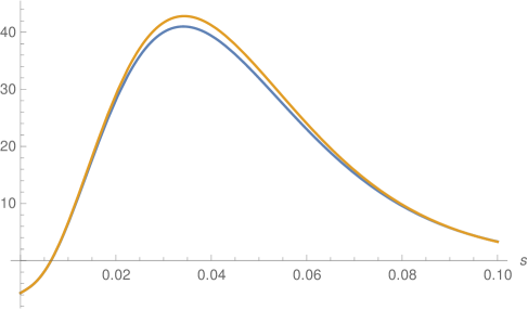
Figure 1: $\frac{1}{s}\,e^{-s(n(n+3)-m(m+1))}\chi_{nm}(s)$ versus $\frac{1}{s}\,e^{-s(n(n+3)-m(m+1))}(O(s^{4})+\tilde{\mu}^{2}O(s))$ as in (4.14) for $n=9,m=4,\mu=0.02$. The negative contribution for small $s$ arises from SUSY breaking due to $\mu\neq 0$.

Then the integral over $s$ can be trivially evaluated. To perform the sum $\sum\limits_{n=1}^{N}\sum\limits_{m=1}^{n-1}$, we can make the following simplifications which are valid for large $n,m$:

$$\chi_{nm}(s)\ \sim\ \dim(n-m,2m)\big{(}(n^{2}-m^{2})^{2}s^{4}-5\tilde{\mu}^{2}s\big{)}$$

$$\dim(n-m,2m)\ \sim\ \frac{2}{3}nm(n^{2}-m^{2})$$ (4.19)

and

$$\frac{1}{(n(n+3)-m(m+1))^{4}}\ \sim\ \frac{1}{(n^{2}-m^{2})^{4}}\ .$$ (4.20)

Approximating the sum by an integral for large $N$, we obtain

$$\Gamma_{\!\textrm{1loop}}\ \stackrel{{\scriptstyle N\to\infty}}{{\sim}}\ -\frac{1}{2}\int_{0}^{N}dn\int_{0}^{n-1}dm\Big{(}\frac{4nm}{n^{2}-m^{2}}-\frac{10}{3}nm\tilde{\mu}^{2}\Big{)}$$

$$\ \sim\ \ -\frac{1}{2}N^{2}\ln N+\frac{5}{24}N^{4}\tilde{\mu}^{2}\ .$$ (4.21)

Here the singularity at $n=m$ (due to the modes with low masses) is just barely avoided, and the main contribution comes from the far UV region $m\lesssim n$. We can check the validity of this approximation by keeping the exact form of the $O(s^{4})+\tilde{\mu}^{2}O(s)$ terms in $\chi_{nm}$ (4.14). This gives

$$\Gamma_{\!\textrm{1loop}}\ \sim\ -\frac{1}{2}N^{2}\left(\ln N-\frac{5}{4}-\ln 2\right)+O(N\ln N)\ +\big{(}\frac{5}{24}N^{4}+O(N^{3})\big{)}\tilde{\mu}^{2}$$

$$\stackrel{{\scriptstyle N\to\infty}}{{\sim}}-\frac{1}{2}N^{2}\ln N+\frac{5}{24}N^{4}\,\frac{\mu^{2}}{r^{2}}$$ (4.22)

in agreement with (4.21). Thus for $\mu=0$, the one-loop contribution gives indeed an attractive potential $\Gamma_{\!\textrm{1loop}}\sim-\frac{1}{2}N^{2}\ln N$, and the factor $N^{2}$ clearly reflects the $N(+1)$ coinciding branes which constitute $S^{4}_{N}$. However for $\mu^{2}>0$, the last term describes a strong repulsive fermionic contribution $\Gamma_{\!\textrm{1loop}}>0$ due to SUSY breaking. In particular, we see that the attractive contribution dominates for $r\to\infty$, while the repulsive contribution dominates for small $r$ as anticipated.

To finally demonstrate the stabilization of $r$, consider the full one-loop effective potential

$$\Gamma_{\rm eff}[r]\ \sim\ \frac{1}{6g^{2}}r^{4}(1+\frac{1}{4}\tilde{\mu}^{2})N^{5}-\frac{1}{2}N^{2}\ln N+\frac{5}{24}N^{4}\tilde{\mu}^{2}$$ (4.23)

for large $N$, cf. figure 2.

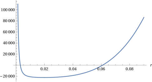
Figure 2: One-loop effective potential $\Gamma_{\rm eff}[r]$ for $\mu=10^{-4},g=1,N=100$.

For given $\mu^{2}>0$, this has a unique stable minimum $r=r_{0}$ at

$$\frac{r^{6}}{\mu^{6}}(1+\frac{\mu^{2}}{8r^{2}}) =\frac{5}{8}\frac{g^{2}}{\mu^{4}}\frac{1}{N}$$ (4.24)

while for $\mu^{2}=0$ the minimum is aways at $r=0$. The parameter

$$\epsilon:=\frac{5}{8N}\frac{g^{2}}{\mu^{4}}$$ (4.25)

determines two scaling regimes:

$$\underline{\epsilon\gg 1}: \qquad\frac{r^{6}}{\mu^{6}}\sim\epsilon\gg 1,\qquad r\sim\big{(}\frac{5g^{2}\mu^{2}}{8N}\big{)}^{\frac{1}{6}}\ \ \qquad\qquad\mbox{Yang-Mills dominated}$$

$$\underline{\epsilon\ll 1}: \qquad\frac{r^{4}}{\mu^{4}}\sim 8\epsilon\ll 1,\qquad r\sim\big{(}\frac{5g^{2}}{N}\big{)}^{\frac{1}{4}}\quad\qquad\qquad\mbox{Mass dominated}$$ (4.26)

We are mainly interested in the Yang-Mills case $\epsilon\gg 1$ which arises for $\mu\to 0$.

Assuming that $\epsilon$ and $g$ is fixed, we can rewrite (4.25) as

$$\mu \sim\Big{(}\frac{5g^{2}}{8}\frac{1}{N\epsilon}\Big{)}^{\frac{1}{4}}\sim N^{-\frac{1}{4}}\ .$$ (4.27)

Together with (2.9), this means that the “physical” radius $R=\frac{1}{2}rN$ of $S^{4}_{N}$ (i.e. the largest eigenvalues) scales as

$$R:=\|X^{a}\|\sim\frac{1}{2}\left\{\begin{array}[]{ll}(\frac{5}{8}\lambda)^{\frac{1}{4}}\epsilon^{-\frac{1}{12}},&\epsilon\gg 1\\[4.30554pt] (5\lambda)^{\frac{1}{4}},&\epsilon\ll 1\end{array}\right.$$ (4.30)

for given $g,\mu^{2}$, where

$$\lambda:=g^{2}N^{3}\sim 6g^{2}{\cal N}$$ (4.31)

is essentially the t’Hooft coupling of the matrix model, where ${\cal N}=\dim{\cal H}_{N}$ is the dimension of the matrices (B.4). Thus the volume $R^{4}$ of the four-sphere scales with the t’Hooft coupling $\lambda$, with a correction factor $\epsilon^{-\frac{1}{3}}$ if $\epsilon\sim\frac{\lambda}{(N\mu)^{4}}\gg 1$. Therefore a large sphere typically arises for large $\lambda$, provided $\mu>0$. It is interesting to recall here the AdS/CFT statement that the supergravity regime is applicable for large t’Hooft coupling; this also supports the validity of our calculations, since the crucial 1-loop effect can be interpreted in terms of supergravity as pointed out above.

Let us evaluate the effective potential at the minimum $r=r_{0}$. For $\epsilon\gg 1$, it is given by

$$\Gamma_{\rm eff}[r_{0}]\ \stackrel{{\scriptstyle\epsilon\gg 1}}{{\sim}}\ \frac{1}{6g^{2}}r_{0}^{4}N^{5}+\frac{5}{24}N^{4}\frac{\mu^{2}}{r_{0}^{2}}-\frac{1}{2}N^{2}\ln N$$

$$\ \sim\frac{5}{16}N^{4}\epsilon^{-\frac{1}{3}}-\frac{1}{2}N^{2}\ln N$$ (4.32)

using (4.26) and (4.25). This maybe positive or negative; a negative energy corresponding to a stable minimum arises if

$$\epsilon >N^{6}(\ln N)^{-3}$$ (4.33)

(roughly). In view of (4.30), this is compatible with the regime of large spheres, e.g. for $\mu\sim N^{-2}$ and $g\sim 1$ we have $\epsilon\sim N^{7}$, $R\sim N^{1/6}$ and $\Gamma_{\rm eff}[r_{0}]<0$.

For $\epsilon\ll 1$, the effective potential at the minimum is

$$\Gamma_{\rm eff}[r_{0}]\ \stackrel{{\scriptstyle\epsilon\ll 1}}{{\sim}}\ \frac{1}{24g^{2}}r^{2}_{0}\mu^{2}N^{5}+\frac{5}{24}N^{4}\frac{\mu^{2}}{r_{0}^{2}}-\frac{1}{2}N^{2}\ln N$$

$$\ \sim\frac{5}{24}N^{4}(8\epsilon)^{-\frac{1}{2}}-\frac{1}{2}N^{2}\ln N$$ (4.34)

This is always positive since $\epsilon\ll 1$ by assumption.

An example for a potential with a negative energy minimum is shown in figure 2 for $\mu\ll 1$. This means that the extended $S^{4}_{N}$ background is preferred over the trivial vacuum. Since the mechanism is expected to apply also in the Minkowski model due to the IR regularization by an imaginary mass term, this might explain the spontaneous generation of 3+1-dimensional geometries found in numerical simulations of the Minkowskian model [17].

4.1 Discussion

The crucial point of the stabilization mechanism is that for small $r$, quantum corrections in the presence of $\mu^{2}>0$ induce a strong repulsive (positive) potential due to SUSY breaking. For large $r$, SUSY becomes almost exact, and the quantum corrections induce an attractive (negative) contribution independent of $r$, in addition to the positive bare potential $\sim O(r^{2})+O(r^{4})$. This leads to a stable minimum at $r_{0}>0$. For $\mu=0$, there is no stabilization at one loop, and the sphere would collapse. This may be (part of) the reason why 4-dimensional geometries have not been observed in Monte-Carlo-simulations of the Euclidean IIB model without mass term [30].

Let us try to assess the validity of the present results. First of all, figure 2 makes clear that the basic mechanism is very robust at one loop. There are two important ingredients: 1) $\Gamma_{\rm eff}\to\infty$ as $r\to 0$, and 2) $\Gamma_{\rm eff}\to\infty$ as $r\to\infty$. Both statements are very robust: for $r\to 0$, the mass term $\mu^{2}X^{2}$ becomes dominant and leads to a strong deviation from supersymmetry, so that the full power of UV divergences kicks in and induces a huge vacuum energy (corresponding to the cosmological constant). On the other hand for $r\to\infty$, the background approaches a stack of $N$ flat branes, with a self-dual background flux. Then quantum corrections are expected to be mild, so that the bare action dominates and contributes $r^{4}N^{5}$. These two effects should be dominant even in the full quantum theory. Therefore the stabilization mechanism is robust.

It is important to see that for large radius, the mechanism is clearly local, and the bare “brane tension” is balanced by the negative vacuum energy; the breaking of translational invariance by the $X^{2}$ term in the bare action is then insignificant. This means that the same mechanism should also apply to other geometries, as long as the curvature is not too large. This is reflected in figure 2, which shows that the effective potential is remarkably flat near the minimum, for large $N$. This means that the precise geometry of the brane is not important. Thus geometric deformations are not suppressed, which is very interesting from the gravity point of view. This will be addressed in future work.

Higher order corrections.

To assess the validity of the one-loop computation, it is useful to view the background as a stack of $N$ spherical noncommutative spheres with “local” Poisson structure $\theta^{\mu\nu}$. Then the fluctuation modes can be viewed in terms of ${\cal N}=4$ $U(N)$ noncommutative Super-Yang-Mills gauge theory with effective coupling constant [13]

$$\frac{1}{4g_{YM}^{2}}=\frac{1}{(2\pi)^{2}g^{2}}{\rm Pf}\theta^{\mu\nu}\sqrt{\det g_{\mu\nu}}\ \sim\ \frac{1}{(2\pi)^{2}g^{2}}r_{N}^{2}\sim\frac{N^{2}}{g^{2}}$$ (4.35)

using ${\rm Pf}\theta^{\mu\nu}\sim r_{N}^{2}$ (2.30) in the $x^{\mu}$ coordinates; note that the scaling factor $r$ drops out here. Hence the higher-order perturbative corrections boil down to a calculation in ${\cal N}=4$ noncommutative $U(N)$ SYM theory, with t’Hooft coupling $g_{YM}^{2}N\sim g^{2}/N$. Therefore the $k$-loop contributions to the potential are expected to be of order $N^{2}(g^{2}/N)^{k-1}$. These generic results are in fact significantly suppressed due to maximal supersymmetry, cf. the discussion in [20] for the case of fuzzy tori. In any case, for $g=O(1)$ the 2- and higher-loop contributions are clearly smaller than the one-loop effective action (4.23), which is at least of order $O(N^{2})$. Therefore we expect that the one-loop results of this paper receive only small perturbative corrections for large $N$. This makes sense, since then the semi-classical geometrical picture applies, so that the semi-classical evaluation of the (super)gravity interaction should be justified. However, due to the (parametrically small) mass parameter $\mu^{2}$ and the associated SUSY breaking, these arguments are only heuristic, and a more careful consideration of possible UV contributions should be given eventually.

Nonperturbatively, the issue is of course much more complicated due to the many possible geometric configurations in the matrix model, as illustrated in the next section. Nevertheless, it seems plausible that for large $N$ where the background becomes almost BPS, the “decay barrier” of the geometry should indeed be large.

4.2 One-loop potential for stacks of fuzzy spheres

The above mechanism is clearly quite general and applies to many similar backgrounds. For comparison, we repeat the computation for a background of $k$ coinciding fuzzy 2-spheres $S^{2}_{N}$, given by

$$X_{i}=r\bar{X}_{i},\qquad[\bar{X}_{i},\bar{X}_{j}]=i\varepsilon_{ijk}\bar{X}_{k},\qquad\sum_{i=1}^{3}\bar{X}_{i}\bar{X}_{i}=\frac{1}{4}N(N+2)\ .$$ (4.36)

The decomposition of the algebra of functions on $S^{2}_{N}$ is ${\cal A}=\oplus_{n=0}^{N-1}(2n)$, where $(n)$ denotes the highest weight representation with Dynkin label $n\in{\mathbb{N}}$ and spin $2j=n$. The Casimir is (keeping the same notation as for $S^{4}_{N}$)

$$C^{2}[\mathfrak{so}(3)](n) =\sum_{a<b\leq 3}{\cal M}_{ab}{\cal M}_{ab}(n)=\frac{1}{4}n(n+2)\ .$$ (4.37)

The bosonic modes have the following (generic) tensor product decomposition

$${\cal A} \in(2)\otimes(n)=(n+2)\oplus(n)\oplus(n-2)$$ (4.38)

and for ${\cal A}_{i}\in(n)$ we have

$$(M_{bc}^{(ad)}\otimes M_{bc}^{(vect)})|_{{\cal A}\in(n+2)} =n$$

$$(M_{bc}^{(ad)}\otimes M_{bc}^{(vect)})|_{{\cal A}\in(n)} =-2$$

$$(M_{bc}^{(ad)}\otimes M_{bc}^{(vect)})|_{{\cal A}\in(n-2)} =-n-2\ .$$ (4.39)

The fermionic modes have the following (generic) tensor product decomposition

$$\Psi \in(1)\otimes(n)=(n+1)\oplus(n-1)$$ (4.40)

and for $\Psi\in(1)\otimes(n)$ we have

$$(M_{bc}^{(ad)}\otimes M_{bc}^{(spin)})|_{\Psi\in(n+1)} =\frac{n}{2}$$

$$(M_{bc}^{(ad)}\otimes M_{bc}^{(spin)})|_{\Psi\in(n-1)} =-\frac{n+2}{2}\ .$$ (4.41)

Then the 1-loop action (4.12) is replaced by

$$\Gamma_{\!\textrm{1loop}}[X]\!=-\frac{1}{2}\int\limits_{0}^{\infty}\frac{ds}{s}\sum_{n=1}^{N-1}e^{-\frac{1}{4}sn(n+2)}\chi_{n}$$ (4.42)

where the “generic” contribution is

$$\chi_{n} =\Big{(}e^{sn}\dim(n+2)+e^{s(-2)}\dim(n)+e^{-s(n+2)}\dim(n-2)+7\dim(n)\Big{)}e^{-\frac{1}{2}s\tilde{\mu}^{2}}$$

$$-2\dim(n)-4\Big{(}e^{\frac{1}{4}s(2n)}\dim(n+1)+e^{\frac{1}{4}s(-2n-4)}\dim(n-1)\Big{)}$$

$$=\chi_{n}^{(0)}(s)+\tilde{\mu}^{2}\chi_{n}^{(1)}(s)+O(\mu^{4})$$ (4.43)

with

$$\chi_{n}^{(0)}(s) =\frac{1}{48}n(n+1)(n+2)(3n^{2}+6n-4)s^{4}+O(s^{5})$$

$$\chi_{n}^{(1)}(s) =-5(n+1)s+O(s^{2}).$$ (4.44)

Keeping the $O(s^{4})+\mu^{2}O(s)$ terms as before and carrying out the sum, we obtain

$$\Gamma_{\!\textrm{1loop}}[S^{2}_{N}]\ \sim\ -\frac{56}{9}+10\frac{\mu^{2}}{r^{2}}\,\ln N$$ (4.45)

in the large $N$ limit. This gets multiplied by $k^{2}$ on a stack of $k$ coincident $S^{2}_{N}$. The bare bosonic action (3.1) for the background $X=r\bar{X}\otimes\mbox{1 \kern-5.89996pt{\rm l}}_{k}$ is

$$S[X]=\frac{1}{g^{2}}r^{4}(2+\tilde{\mu}^{2})N^{2}(N+2)k$$ (4.46)

and we obtain the full one-loop large $N$ effective potential

$$\Gamma_{\rm eff}[r] =\frac{1}{g^{2}}r^{4}(2+\tilde{\mu}^{2})N^{3}k+\big{(}-\frac{56}{9}+10\frac{\mu^{2}}{r^{2}}\ln N\big{)}k^{2}\ .$$ (4.47)

For given $\mu^{2}>0$, this has a unique stable minimum $r=r_{0}$ at

$$\frac{r^{6}}{\mu^{6}}(1+\frac{\mu^{2}}{4r^{2}}) =\frac{5}{2}\frac{k\ln N}{N^{3}}\frac{g^{2}}{\mu^{4}}$$ (4.48)

while for $\mu^{2}=0$ the minimum is aways at $r=0$. Now the parameter

$$\tilde{\epsilon}:=\frac{5}{2}\frac{k\ln N}{N^{3}}\frac{g^{2}}{\mu^{4}}$$ (4.49)

determines two scaling regimes:

$$\underline{\tilde{\epsilon}\gg 1}: \qquad\frac{r^{6}}{\mu^{6}}\sim\tilde{\epsilon}\gg 1,\qquad r\sim\big{(}\frac{5g^{2}\mu^{2}}{2}\frac{k\ln N}{N^{3}}\big{)}^{\frac{1}{6}}\ \ \qquad\qquad\mbox{Yang-Mills dominated}$$

$$\underline{\tilde{\epsilon}\ll 1}: \qquad\frac{r^{4}}{\mu^{4}}\sim 4\tilde{\epsilon}\ll 1,\qquad r\sim\big{(}10g^{2}\frac{k\ln N}{N^{3}}\big{)}^{\frac{1}{4}}\quad\qquad\qquad\mbox{Mass dominated}$$ (4.50)

We can evaluate the effective potential at the minimum. For $\tilde{\epsilon}\gg 1$, it is given by

$$\Gamma_{1-loop} \stackrel{{\scriptstyle\epsilon\gg 1}}{{\sim}}\frac{2}{g^{2}}r^{4}N^{3}k+\big{(}-\frac{56}{9}+10\ln N\frac{\mu^{2}}{r^{2}}\big{)}k^{2}$$

$$\sim 5\epsilon^{-\frac{1}{3}}k^{2}\big{(}1+2\ln N\big{)}-\frac{56}{9}k^{2}$$ (4.51)

using (4.50) and (4.49), which is negative if

$$\tilde{\epsilon} >8(1+2\ln N)^{3}$$ (4.52)

(roughly). For $\tilde{\epsilon}\ll 1$, the effective potential at the minimum is always positive for the same reason as in $S^{4}_{N}$.

Comparing with (4.32), we see that for some parameter range (e.g. as in figure 2 and $k=1$), $S^{4}_{N}$ has indeed a lower one-loop potential than a single fuzzy $S^{2}$. However, it is easy to see from (4.47) that if we vary $k$ for fixed dimension ${\cal N}=kN$, then $\Gamma_{\rm eff}$ for $S^{2}_{N}$ is minimized for large $k$. This means that the quantum number $N$ for a single fuzzy sphere is preferred to be small, presumably $N=2$, while $k$ is large. This would suggest that the semi-classical geometries with large $N$ may ultimately be unstable. On the other hand, the 1-loop approximation is more reliable in the large $N$ case where the background becomes almost BPS, and the “decay barrier” is expected to be large. These issues are left for future investigations.

5 Conclusion

We have performed a detailed one-loop computation for fuzzy $S^{4}_{N}$ in the IIB matrix model with a (small) positive mass $\mu^{2}$, and determined the one-loop effective potential for the radius $r$. We have found a robust stabilization mechanism for $S^{4}_{N}$ and similar fuzzy spaces, as long as $\mu^{2}>0$. This can be understood in terms of a negative contribution to the potential attributed to supergravity, balanced by a positive contribution due to the SUSY breaking effect of $\mu^{2}$. The latter is important only for small $r$, leading to a robust stabilization mechanism. For suitable parameters the radius becomes large, and the energy can be negative for small $\mu^{2}$. We also argue (somewhat superficially) that higher-order perturbative corrections should be small for large $N$. This suggests that large, semi-classical spheres should indeed exist as meta-stable configurations in the model. However, the mechanism is not restricted to the fuzzy $S^{4}_{N}$ geometry.

This result is very interesting in the context of recent numerical results on the genesis of 3+1-dimensional space-time in the Minkowskian IIB model [17]. Our mechanism is expected to work also in the Minkowski case, and it might help to explain and to interpret these numerical results. In fact, an IR regularization of the IIB model is necessary in the Minkowski case, which can be interpreted [17] as a Wick rotation of the present mass term, ensuring also the Feynman $i\varepsilon$ prescription. This motivates to introduce a (parametrically small) mass term also in the Euclidean model. It would therefore be very interesting to reconsider the Euclidean model numerically in the presence of such a mass term. Even if no spontaneous generation of 4-dimensional spaces might happen due to non-perturbative effects, the present background should at least be metastable.

At the non-perturbative level, the situation is clearly much more complicated. We consider the case of $k$ coinciding fuzzy 2-spheres at one loop, where the same mechanism applies in principle. It turns out that configurations with many small spheres are preferred at the one-loop level. However, this result is not expected to be reliable beyond one loop.

We also find that the effective potential for the radius of $S^{4}_{N}$ is remarkably flat near the minimum, for large $N$. This means that geometric deformations are not suppressed, which strongly suggests that some type of gravity with massless modes should arise on the background. Due to the manifest Lorentz- (or rather Euclidean) invariance, the emergence of 4-dimensional general relativity on such backgrounds in matrix models seems natural, cf. [13, 15]. Since the vacuum energy is fully incorporated (in fact it is the essential ingredient of the stabilization mechanism), one is tempted to speculate that this might shed light on the mysteries of dark energy and the cosmological constant. However, this can only be addressed in a meaningful way once the fluctuation modes on $S^{4}_{N}$ and their physical significance are understood. These include in particular a tower of massless higher spin modes, whose fate remains to be determined. All these are interesting topics for further work.

Acknowledgements.

I would like to thank T. Chatzistavrakidis, D. O’Connor, M. Hanada, S. Ramgoolam, A. Tsuchiya and C-S. Chu for useful discussions, and J. Zahn and J. Karczmarek for related collaboration and correspondence. This work was primarily supported by the Austrian Science Fund (FWF) grant P24713, and in part by the Action MP1405 QSPACE from the European Cooperation in Science and Technology (COST).

Appendix A Semi-classical geometry: ${\mathbb{C}}P^{3}$ as $S^{2}$ bundle over $S^{4}$

The semi-classical geometry of $S^{4}_{N}$ is obtained by recognizing (2.14) as fuzzy version of the Hopf map

$$X^{i}\sim x^{i}:\quad{\mathbb{C}}P^{3}\to S^{4}\subset{\mathbb{R}}^{5}$$ (A.1)

which is defined as follows. We view ${\mathbb{C}}^{4}$ as fundamental representation of $SU(4)$. Acting on a reference point $z^{(0)}=(1,0,0,0)\in{\mathbb{C}}^{4}$, $SU(4)$ sweeps out the 7-sphere $S^{7}\subset{\mathbb{R}}^{8}\cong{\mathbb{C}}^{4}$. We can then define the Hopf map

$$S^{7} \to S^{4}\ \subset{\mathbb{R}}^{5}$$ (A.2)

$$z^{\alpha} \mapsto x_{i}=z_{\alpha}^{*}(\gamma_{i})^{\alpha}_{\ \beta}z^{\beta}\equiv\langle z|\gamma_{i}|z\rangle$$ (A.3)

where $\gamma_{i}$ are the $\mathfrak{so}(5)$ gamma matrices. It is easy to verify that $R^{2}=\sum_{i=1}^{5}x_{i}^{2}=1$, so that the rhs is indeed in $S^{4}$. Since the overall phase of $z_{i}$ drops out in (A.3), this defines a map of ${\mathbb{C}}P^{3}\cong S^{7}/U(1)$ into $S^{4}$. It is thus useful to re-interpret (A.3) as

$$x_{i}:\quad{\mathbb{C}}P^{3}\ \to S^{4}\subset{\mathbb{R}}^{5}$$

$$|z\rangle\langle z| \mapsto\langle z|\gamma_{i}|z\rangle=tr(|z\rangle\langle z|\gamma_{i})\ .$$ (A.4)

Here $|z\rangle\in{\mathbb{C}}^{4}$, and ${\mathbb{C}}P^{3}$ is identified with the space of rank one projectors $|z\rangle\langle z|$. Using $\gamma_{5}=\begin{pmatrix}\mbox{1 \kern-5.89996pt{\rm l}}_{2}&0\\ 0&-\mbox{1 \kern-5.89996pt{\rm l}}_{2}\end{pmatrix}$ in the Weyl basis, we have $x_{i}(p)=(0,0,0,0,1)$ at the reference point $p\in S^{4}$, with stabilizer

$$H=\{h;[h,\gamma_{5}]=0\}\ \subset SO(5)$$ (A.5)

given by

$$H\cong SU(2)_{R}\times SU(2)_{L}=SO(4)$$

where $SU(2)_{L}$ acts on the $+1$ eigenspace of $\gamma_{5}$. The fiber over $p\in S^{4}$ is determined by

$$\langle z|\gamma^{5}|z\rangle=1,$$ (A.6)

which using the explicit form of $\gamma_{5}$ is given by

$$|z_{1}|^{2}+|z_{2}|^{2}=1\ .$$ (A.7)

This defines $S^{3}$, which modulo the $U(1)$ phase (passing to ${\mathbb{C}}P^{3}$) reduces to $S^{2}$. Hence ${\mathbb{C}}P^{3}$ is an $S^{2}$-bundle over $S^{4}$, and the $S^{2}$ fiber over $z^{(0)}$ is obtained by acting with $SU(2)_{L}$ on $z^{(0)}$. In contrast, $SU(2)_{R}\times U(1)\subset H$ is in the stabilizer of $z^{(0)}$, hence it acts trivially on ${\mathbb{C}}P^{3}$.

Some further remarks on the group theory are in order. The embedding $SO(5)\subset SO(6)$ is given by extending the $SO(5)$ generators $M_{ij},\ i,j\leq 5$ by $M_{i6}$. This embedding is not regular, i.e. the $SO(5)$ roots are not a subset of the $SO(6)$ roots. However, the two commuting $SU(2)_{L},SU(2)_{R}\subset SO(5)\subset SU(4)$ (correspond to the long roots of $SO(5)$) can be identified with the simple roots $\alpha_{1},\alpha_{3}$ of $SU(4)\cong SO(6)$ which are orthogonal:

$$SU(2)_{R}\equiv SU(2)_{\alpha_{1}},\qquad SU(2)_{L}\equiv SU(2)_{\alpha_{3}}\ .$$ (A.8)

The roots (and the weight lattice) of $SO(5)$ are then obtained by projecting the roots (resp. the weights) of $SU(4)$ along $\Lambda_{2}$ onto the $\alpha_{1}\alpha_{3}$ - plane, see figure 3.

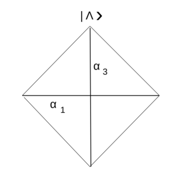
Figure 3: Weight tetrahedron of ${\cal H}_{N}$ with highest weight $\Lambda=(0,0,N)$ of $\mathfrak{su}(4)$ projected along $\Lambda_{2}$ to the weight space of $\mathfrak{so}(5)$.

In particular, $SU(2)_{R}$ acts trivially on the highest weight (coherent) state $|\Lambda\rangle$ of ${\cal H}_{N}$, while $SU(2)_{L}=SU(2)_{\alpha_{3}}$ acts non-trivially and generates a $N+1$-dimensional representation at the edge of the weight tetrahedron of ${\cal H}_{N}$. This gives precisely the fuzzy $S^{2}_{N+1}$ corresponding to the fiber. Hence at each point of $S^{4}$ there is an “internal” $SU(2)_{L}\subset H$ which rotates the coherent states on $S^{2}$ over the same point of $S^{4}$.

Appendix B Some representation theory

Representations of $\mathfrak{su}(4)$ are labeled by the Dynkin indices of their highest weights. Weyls dimension formula gives

$$\dim(n,0,n)=\frac{1}{12}(n+1)^{2}(n+2)^{2}(2n+3)\ .$$ (B.1)

For $\mathfrak{so}(5)$, let $\Lambda=n\Lambda_{1}+n\Lambda_{2}$ where $\alpha_{1}$ is the long root and $\alpha_{2}$ the short root. The dimension of $(n,m)$ is given by

$$\dim(n,m)=\frac{1}{6}(n+1)(m+1)(n+m+2)(2n+m+3)$$ (B.2)

or

$$\dim(n-m,2m)=\frac{1}{6}(2n+3)(2m+1)(n+m+2)(n-m+1)\ .$$ (B.3)

In particular,

$$\dim{\cal H}_{N}=\dim(0,N)=\frac{1}{6}(N+1)(N+2)(N+3)\ .$$ (B.4)

For example,

$$\dim(1,0) =5,\quad\dim(0,1)=4,\quad\dim(0,2)=10\ .$$ (B.5)

In particular $(0,2)$ is the adjoint. One can decompose $(n,0,n)$ of $\mathfrak{su}(4)$ into irreps of $\mathfrak{so}(5)$. It is not hard to see that

$$(n,0,n)=(n,0)\oplus(n-1,2)\oplus(n-2,4)\oplus...\oplus(0,2n)$$ (B.6)

These are given by irreducible expressions of the type $P_{n}(X)\in(n,0),\ P_{n-1}(X){\cal M}\in(n-1,2),\ P_{n-2}(X){\cal M}{\cal M}\in(n-2,4)$ and so on.

References

- [1] J. Madore, “The Fuzzy sphere,” Class. Quant. Grav. 9, 69 (1992).
- [2] J. Hoppe, ”Quantum theory of a massless relativistic surface and a two-dimensional bound state problem“, PH D thesis, MIT 1982;
- [3] P. M. Ho and M. Li, “Fuzzy spheres in AdS / CFT correspondence and holography from noncommutativity,” Nucl. Phys. B 596, 259 (2001) [hep-th/0004072].
- [4] D. Jurman and H. Steinacker, “2D fuzzy Anti-de Sitter space from matrix models,” JHEP 1401 (2014) 100 [arXiv:1309.1598 [hep-th]].
- [5] H. Grosse, C. Klimcik and P. Presnajder, “On finite 4-D quantum field theory in noncommutative geometry,” Commun. Math. Phys. 180, 429 (1996) doi:10.1007/BF02099720 [hep-th/9602115].
- [6] J. Castelino, S. Lee and W. Taylor, “Longitudinal five-branes as four spheres in matrix theory,” Nucl. Phys. B 526, 334 (1998) [hep-th/9712105].
- [7] S. Ramgoolam, “On spherical harmonics for fuzzy spheres in diverse dimensions,” Nucl. Phys. B 610, 461 (2001) [hep-th/0105006].
- [8] P. M. Ho and S. Ramgoolam, “Higher dimensional geometries from matrix brane constructions,” Nucl. Phys. B 627, 266 (2002) [hep-th/0111278].
- [9] Y. Kimura, “Noncommutative gauge theory on fuzzy four sphere and matrix model,” Nucl. Phys. B 637, 177 (2002) [hep-th/0204256].
- [10] J. Medina and D. O’Connor, “Scalar field theory on fuzzy S**4,” JHEP 0311, 051 (2003) [hep-th/0212170].
- [11] Y. Abe, “Construction of fuzzy S**4,” Phys. Rev. D 70, 126004 (2004) [hep-th/0406135].
- [12] P. Valtancoli, “Projective modules over the fuzzy four sphere,” Mod. Phys. Lett. A 17, 2189 (2002) [hep-th/0210166].
- [13] H. Steinacker, “Emergent Geometry and Gravity from Matrix Models: an Introduction,” Class. Quant. Grav. 27, 133001 (2010) [arXiv:1003.4134 [hep-th]].
- [14] H. Steinacker, “Gravity and compactified branes in matrix models,” JHEP 1207, 156 (2012) [arXiv:1202.6306 [hep-th]].
- [15] J. Heckman and H. Verlinde, “Covariant non-commutative space–time,” Nucl. Phys. B 894, 58 (2015) [arXiv:1401.1810 [hep-th]].
- [16] N. Ishibashi, H. Kawai, Y. Kitazawa and A. Tsuchiya, “A Large N reduced model as superstring,” Nucl. Phys. B 498, 467 (1997) [hep-th/9612115].
- [17] S. -W. Kim, J. Nishimura, and A. Tsuchiya, “Expanding (3+1)-dimensional universe from a Lorentzian matrix model for superstring theory in (9+1)-dimensions,” Phys. Rev. Lett. 108 (2012) 011601 [arXiv:1108.1540 [hep-th]]; Y. Ito, S. -W. Kim, Y. Koizuka, J. Nishimura and A. Tsuchiya, “A renormalization group method for studying the early universe in the Lorentzian IIB matrix model,” arXiv:1312.5415 [hep-th]; S. W. Kim, J. Nishimura and A. Tsuchiya, “Late time behaviors of the expanding universe in the IIB matrix model,” JHEP 1210, 147 (2012) [arXiv:1208.0711 [hep-th]].
- [18] T. Azuma, S. Bal, K. Nagao and J. Nishimura, “Absence of a fuzzy S**4 phase in the dimensionally reduced 5-D Yang-Mills-Chern-Simons model,” JHEP 0407, 066 (2004) [hep-th/0405096].
- [19] I. Chepelev and A. A. Tseytlin, “Interactions of type IIB D-branes from D instanton matrix model,” Nucl. Phys. B 511 (1998) 629 [hep-th/9705120].
- [20] S. Bal, M. Hanada, H. Kawai and F. Kubo, “Fuzzy torus in matrix model,” Nucl. Phys. B 727, 196 (2005) [hep-th/0412303].
- [21] H. S. Snyder, “Quantized space-time,” Phys. Rev. 71, 38 (1947); C. N. Yang, “On quantized space-time,” Phys. Rev. 72, 874 (1947).
- [22] M. Fabinger, “Higher dimensional quantum Hall effect in string theory,” JHEP 0205, 037 (2002) [hep-th/0201016].
- [23] D. Karabali and V. P. Nair, “Quantum Hall effect in higher dimensions, matrix models and fuzzy geometry,” J. Phys. A 39, 12735 (2006) [hep-th/0606161].
- [24] J. Medina, I. Huet, D. O’Connor and B. P. Dolan, “Scalar and Spinor Field Actions on Fuzzy : fuzzy as a bundle over ,” JHEP 1208, 070 (2012) [arXiv:1208.0348 [hep-th]].
- [25] A. P. Balachandran, B. P. Dolan, J. H. Lee, X. Martin and D. O’Connor, “Fuzzy complex projective spaces and their star products,” J. Geom. Phys. 43, 184 (2002) [hep-th/0107099].
- [26] U. Carow-Watamura, H. Steinacker and S. Watamura, “Monopole bundles over fuzzy complex projective spaces,” J. Geom. Phys. 54, 373 (2005) [hep-th/0404130].
- [27] S. Doplicher, K. Fredenhagen and J. E. Roberts, “The Quantum structure of space-time at the Planck scale and quantum fields,” Commun. Math. Phys. 172 (1995) 187 [hep-th/0303037].
- [28] J. L. Karczmarek and K. H. C. Yeh, “Noncommutative spaces and matrix embeddings on flat ,” arXiv:1506.07188 [hep-th].
- [29] D. N. Blaschke and H. Steinacker, “On the 1-loop effective action for the IKKT model and non-commutative branes,” JHEP 1110, 120 (2011) [arXiv:1109.3097 [hep-th]]; A. Chatzistavrakidis, H. Steinacker and G. Zoupanos, “Intersecting branes and a standard model realization in matrix models,” JHEP 1109, 115 (2011) [arXiv:1107.0265 [hep-th]].
- [30] J. Nishimura, T. Okubo and F. Sugino, “Systematic study of the SO(10) symmetry breaking vacua in the matrix model for type IIB superstrings,” JHEP 1110, 135 (2011) [arXiv:1108.1293 [hep-th]].