HATS-17b: A TRANSITING COMPACT WARM JUPITER IN A 16.3 DAYS CIRCULAR ORBIT

Abstract

We report the discovery of HATS-17b, the first transiting warm Jupiter of the HATSouth network. HATS-17b transits its bright (V=12.4) G-type ($M_{\star}$=$1.131\pm 0.030$ $M_{\sun}$, $R_{\star}$=$1.091_{-0.046}^{+0.070}$ $R_{\sun}$) metal-rich ([Fe/H]=$+0.3$ dex) host star in a circular orbit with a period of $P$=$16.2546$ days. HATS-17b has a very compact radius of $0.777\pm 0.056$ $R_{\rm J}$ given its Jupiter-like mass of $1.338\pm 0.065$ $M_{\rm J}$. Up to 50% of the mass of HATS-17b may be composed of heavy elements in order to explain its high density with current models of planetary structure. HATS-17b is the longest period transiting planet discovered to date by a ground-based photometric survey, and is one of the brightest transiting warm Jupiter systems known. The brightness of HATS-17 will allow detailed follow-up observations to characterize the orbital geometry of the system and the atmosphere of the planet.

1. Introduction

The detection of numerous extrasolar giant planets has brought forth several theoretical challenges regarding their formation, structure and evolution. One of these challenges arises from the fact that for over 20 years, radial velocity (RV) surveys have been discovering large number of giant planets found to orbit their host stars at short distances ($<1$ AU), where they are highly unlikely to be formed. Hot Jupiters having semi-major axes of $\sim$0.03 AU, are the most extreme cases. Short period giant planets are thought to be formed at several AUs, beyond the so-called snow line, where sufficient solid material is available to build $\sim$10 $M_{\earth}$ cores that accrete their gaseous envelopes from the protoplanetary disc before it is dispersed (e.g., Rafikov, 2006). The subsequent inward migration can be produced by the exchange of angular momentum with the same protoplanetary disc (Goldreich & Tremaine, 1980) and/or by gravitational interactions with other stellar or planetary bodies which produce high eccentricity migration mechanisms, in which eccentricities are excited and the semi-major axis decreases due to tidal interactions with the star (Rasio & Ford, 1996; Wu & Lithwick, 2011; Fabrycky & Tremaine, 2007; Petrovich, 2015). These two migration mechanisms predict different end products. While disc migration should produce circular orbits in which the angular momentum vector of the orbit is aligned with the spin of the star, high eccentricity migration mechanisms can produce planets with a broad distribution of eccentricities and misalignment angles.

Transiting extrasolar planets (TEPs) are fundamental objects for constraining migration scenarios, because the measurement of the Rossiter-McLaughlin effect (Rossiter, 1924; McLaughlin, 1924) allows the determination of the sky-projected angle between the orbital and stellar spins. This angle has been determined for several transiting hot Jupiters showing that while most of the systems have well aligned prograde orbits, an important fraction of them is found to present measurable misalignments (Hébrard et al., 2008; Queloz et al., 2010; Winn et al., 2010). Hot Jupiters, however, are not optimal systems for discriminating between migration mechanisms. The tidal or magnetic interactions with the host star which can arise due to their extremely close-in orbits can be responsible for not only circularising the orbit but also potentially realigning the spin of the star with the orbit of the planet and thereby affecting the final state of the system (Dawson, 2014). Transiting giant planets with larger semi-major axes ($a>0.1$ AU), on the other hand, do not suffer from strong interactions with their stars and can be used for measuring a more pristine final state of the migration process.

While TEPs can be used to refine the geometrical configuration of the orbits, arguably their most important feature is that their radii can be derived from the transit depth if the radii of the stellar hosts are known. The estimation of the radius, coupled with the measurement of the planetary mass from RV observations, allows the computation of the bulk density of the planet and the possibility of inferring properties about its internal structure and composition. Another theoretical challenge arose with the discovery of the first transiting extrasolar planets. While theories of giant planet evolution predicted $\approx 1R_{\rm J}$ for planets with masses $\approx 1M_{\rm J}$, ages above 1Gyr and no cores (Burrows et al., 2007), observations of close-in transiting giant planets revealed a broad distribution of planetary radii, with some of them reaching even twice the radius of Jupiter, like HAT-P-32b (Hartman et al., 2011). Others had radii more compact than expected from theoretical models without solid cores, like WASP-59b with $R_{P}$=0.78$R_{\rm J}$ (Hébrard et al., 2013).

The origin of these anomalies in the measured radii of giant exoplanets have been extensively investigated, but there are no conclusive theories that are able to explain simultaneously the variety of systems. A central solid core is commonly invoked to explain the radii of compact giant planets, while the proximity of the planets to their stellar hosts is probably responsible of generating the inflated planets via a variety of mechanisms including extra power deposited at some depth via, e.g., tidal or radiative heating mechanisms, enhanced atmospheric opacities, suppression of convective heat loss, among others (for a review see Spiegel & Burrows, 2013). The principal problem of favouring one inflating mechanism over another comes from the degeneracies in the modelled radius that arise from the unknown mass of the central core. Kovács et al. (2010) found that the inflation of the radius stops being efficient for incident stellar fluxes weaker than $\langle F\rangle\approx 2\times$10⁸ erg s^-1 cm^-2 (see also Demory & Seager, 2011). Detections of giant planets with irradiation values below this limit are very valuable because the interior structure of the planet can be estimated without assumptions about extra energy sources. Furthermore, the distribution of core masses determined for weakly irradiated giant planets can then be extrapolated to highly irradiated planets to constrain inflation mechanisms.

As stated above, giant TEPs with moderately long orbital periods (warm Jupiters) are unique test objects for validating structure and migrations theories. However, from the total of $\approx 1900$ confirmed or validated planets discovered to date, only 23 transiting planets have $P>10$ days, $R_{P}>0.5$ $R_{\rm J}$ and measured masses greater than 0.25 $M_{\rm J}$. Moreover, most of these interesting systems were discovered with the space based missions Kepler and CoRoT around faint host stars ($V>14$) hindering the measurement of precise RV variations, and limiting future detailed follow-up observations.

On the other hand, the detection of transiting warm Jupiters from the ground is a challenging task. Only two such planets with $P>10$ days are known, originally discovered by RV programs and then later found to transit. These are: HD17156 with $P=22.6$ days (Fischer et al., 2007) and HD80606 with $P=115$ days (Naef et al., 2001). The small number of detections is due to the fact that the transit probability decreases inversely with the semi-major axis. Ground based transit surveys can deal in principle with this low probability problem by monitoring many more stars than the RV programs do, but the diurnal cycle strongly limits the recovery of $P>10$ days planets for common one-site based surveys. The use of longitudinal networks of telescopes is a way of counteracting the limitations imposed by the diurnal cycle. Indeed, the transiting extrasolar planet with the longest period discovered previous to the present study by a ground based transit survey was HAT-P-15b (Kovács et al., 2010) with $P=10.8$ days. This system was detected by the two-site-based HATNet survey (Bakos et al., 2004).

One of the main goals of the HATSouth survey (Bakos et al., 2013) is to expand the parameter space of well characterized transiting planets around moderately bright stars. The first results in this regard have started to appear. HATS-6b (Hartman et al., 2015) is one of only four transiting giant planets discovered around stars with masses $M_{\star}<0.6M_{\sun}$, while HATS-7b (Bakos et al., 2015) and HATS-8b (Bayliss et al., 2015) are now two among the handful of well characterized transiting super Neptunes. Having three locations with large longitude separation in the southern hemisphere, the HATSouth survey is able to monitor, almost continuously, selected fields on the sky for $\sim 4$ months per year, substantially increasing the probability of detecting transiting extrasolar planets with periods longer than 10 days (Bakos et al., 2013). In this paper we present the discovery of HATS-17b, the first transiting warm Jupiter of the HATSouth survey. With an orbital period of $P\sim 16.3$ days, it is the longest period transiting extrasolar planet discovered by a ground-based photometric survey.

The paper is structured as follows. In §2 we describe the photometric and spectroscopic observations that allowed the discovery and confirmation of HATS-17b. In §3 we explain the tools that were used to estimate the physical parameters of HATS-17b and its host star. Finally, in §4 we place the physical properties of HATS-17b in the context of the transiting exoplanets previously detected and outline possible follow-up observations for further characterizing this system.

2. Observations

2.1. Photometry

2.1.1 Photometric detection

The star HATS-17 (Table 4) was observed by HATSouth instruments between UT 2011 April 26 and UT 2012 July 31 using the HS-2, HS-4, and HS-6 units at LCO in Chile, the H.E.S.S. site in Namibia, and SSO in Australia, respectively. The number of observations obtained with each instrument, effective cadence, and photometric precision are listed in Table 1. The data were reduced to trend-filtered light curves using the aperture photometry procedure described by Penev et al. (2013) and making use of External Parameter Decorrelation (EPD; Bakos et al., 2010) and the Trend Filtering Algorithm (TFA; Kovács et al., 2005) to remove systematic variations. We searched for transits using the Box-fitting Least Squares (BLS; Kovács et al., 2002) algorithm, and detected a $P=16.2546{}$ day periodic transit signal in the light curve of HATS-17 (Figure 1; the data are available in Table 2).

Table 1 Summary of Photometric Observations of HATS-17.

Facility/Field	Date Range	Number of Points	Median Cadence	Filter	Precision
			(seconds)		mmag
HS-2/G700 (LCO)	2011 Apr–2012 Jul	4579	292	$r$	5.8
HS-4/G700 (HESS)	2011 Jul–2012 Jul	3759	301	$r$	6.4
HS-6/G700 (SSO)	2011 May–2012 Jul	1499	300	$r$	6.5
PEST 0.3 m (Perth, AU)	2015 Apr 26	215	132	$R_{C}$	2.4
LCOGT 1 m/sinistro (CTIO)	2015 May 13	54	105	$i$	1.3
Swope 1 m/e2v (LCO)	2015 May 29	141	129	$i$	3.8
Swope 1 m/e2v (LCO)	2015 Jul 17	79	99	$i$	1.6
LCOGT 1 m/sinistro (CTIO)	2015 Jul 17	71	162	$i$	0.8

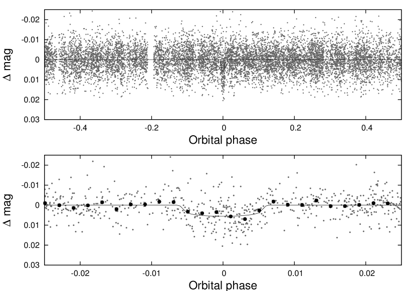
Figure 1.— Unbinned instrumental $r$ band light curve of HATS-17 folded with the period $P=16.2546107$ days resulting from the global fit described in Section 3. The solid line shows the best-fit transit model (see Section 3). In the lower panel we zoom-in on the transit; the dark filled points here show the light curve binned in phase using a bin-size of 0.002. The signal is consistent with flat-bottom transit with a depth of 5 mmag.

2.1.2 Photometric follow-up

Given the quality of the HATSouth detection, follow-up observations of the transit were required in order to confirm that the signal is compatible with a transiting planet, and to precisely determine the physical parameters of the system.

Due to the long period of the discovered transit signal and the long duration of the transits (5.2 hours), the photometric follow-up for this kind of TEP candidate brings more difficulties than the ones presented in more typical ($P<5$ days) candidates. For this reason a high priority photometric follow-up campaign for HATS-17 started only after the spectroscopic observations described in Section 2.2 showed an orbital variation in RV in phase with the photometric ephemeris.

The first photometric follow-up light curve of this system was obtained with the 0.3 m Perth Exoplanet Survey Telescope (PEST) located near Perth. The unbinned precision of 2.5 mmag allowed the measurement of a full $\approx 5$ mmag flat-bottom transit.

Another two partial transits were then acquired with the LCOGT 1 m telescope network, specifically with the telescope at Cerro Tololo Inter-American Observatory (CTIO), and with the Swope 1 m coupled with the e2v camera at Las Campanas Observatory (LCO). The former registered only the egress of the transit which was helpful in refining the ephemeris of the system, while the latter obtained one ingress and part of the transit but the weather conditions were suboptimal and did not allow for a substantial improvement of the measured transit parameters.

Finally, two partial transits of the same event were measured with high photometric precision ($\approx 1$ mmag) in one of the last chances to observe it during the season. The observations were performed with the same two telescopes that registered the previous partial transits and they obtained a fraction of the bottom part of the transit and the egress. These observations revealed a clear transit with a depth of $\approx 6$ mmag and improved substantially the precision of the measured transit parameters.

All the photonetric observations are summarized in Table 1. Table 2 provides the light curve data, while the light curves are compared to our best-fit model in Figure 2. All the facilities used for high precision photometric follow-up have been previously used by HATSouth; the instrument specifications, observation strategies and adopted reduction procedures can be found in Zhou et al. (2014), Bakos et al. (2015) and Bayliss et al. (2015) for PEST, LCOGT 1 m/sinistro (CTIO), and Swope 1 m/e2v, respectively. Given that there were no evident close companions to HATS-17, all photometric follow-up observations were acquired with defocusing.

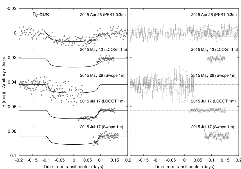
Figure 2.— Left: Unbinned follow-up transit light curves of HATS-17. The dates, filters and instruments used for each event are indicated. Curves after the first are shifted for clarity. Our best fit is shown by the solid lines. Right: Residuals from the fits in the same order as the curves at left.

Table 2Differential photometry of HATS-17

BJD	Mag	$\sigma_{\rm Mag}$	Mag(orig)	Filter	Instrument
(2 400 000$+$)
$56123.25166$	$-0.00660$	$0.00285$	$\cdots$	$r$	HS
$56074.48974$	$0.00167$	$0.00334$	$\cdots$	$r$	HS
$56123.25650$	$0.00042$	$0.00287$	$\cdots$	$r$	HS
$56074.49324$	$0.00716$	$0.00339$	$\cdots$	$r$	HS
$56123.26027$	$-0.00035$	$0.00284$	$\cdots$	$r$	HS
$56074.49672$	$-0.00865$	$0.00337$	$\cdots$	$r$	HS
$56123.26373$	$-0.00323$	$0.00289$	$\cdots$	$r$	HS
$56074.50208$	$-0.00251$	$0.00346$	$\cdots$	$r$	HS
$56123.26876$	$-0.00040$	$0.00286$	$\cdots$	$r$	HS
$56074.50592$	$0.00139$	$0.00342$	$\cdots$	$r$	HS

Note. — This table is available in a machine-readable form in the online journal. A portion is shown here for guidance regarding its form and content. The data are also available on the HATSouth website at http://www.hatsouth.org.

2.2. Spectroscopy

An extensive follow-up campaign is required for validating the planetary nature of HATSouth transiting candidates. Transit-like signals in the light curves can be produced by artifacts in the data or different configurations of stellar eclipsing binaries and background stars. Spectroscopic observations are used for characterizing the properties of the star and to determine the mass and orbital parameters of the planets from RV curves.

The first spectroscopic observation of HATS-17 was carried out by the WiFeS instrument on the ANU 2.3 m telescope at SSO (Dopita et al., 2007). A single low resolution (R=3000) spectrum was enough for a first estimation of the stellar parameters of HATS-17. Following the reductions and analysis procedures detailed in Bayliss et al. (2013), the computed stellar atmospheric parameters were $T_{\rm eff}=5315\pm 300$ K, $\log{g}=4.4\pm 0.3$ dex and $\rm[Fe/H]=-0.5\pm 0.5$ dex. After HATS-17b was identified as a single-lined G-type dwarf, five additional R=7000 spectra were obtained with the same instrument in order to measure RV variations. These five RV points were consistent with no variation at the $\sim$2 $\rm km\,s^{-1}$ level, which shows that the observed photometric signal is not produced by an unblended eclipsing stellar mass companion.

Once HATS-17 passed the reconnaissance spectroscopy filter of our follow-up structure, further spectroscopic characterisation of the HATS-17 system was performed with facilities capable of measuring RV variations produced by the gravitational tug of a giant planet mass companion. Several high resolution spectra were acquired with three spectrographs installed in the ESO La Silla observatory. We obtained 11 spectra using HARPS at the ESO 3.6 m telescope, 8 spectra using CORALIE (Queloz et al., 2001) at the Euler 1.2 m telescope and 2 spectra with FEROS (Kaufer & Pasquini, 1998) at the MPG 2.2 m telescope. The data for these 3 instruments were reduced and analysed with an automated pipeline described in Jordán et al. (2014) that processes in an homogeneous and robust manner data of echelle spectrographs. Besides the reduced spectra, this pipeline delivers precise RV measurements, bisector span (BS) values from the cross-correlation peak and an estimation of the stellar atmospheric parameters. RV and BS values are presented in Table 3 with their corresponding uncertainties. As shown in the top panel of Figure 3, the RV measurements phase cleanly with the photometric ephemeris with an amplitude compatible with the one produced by a Jovian planet in an almost circular orbit. The middle panel of Figure 3 shows the residuals of the measured RV values and the best fit model, while the bottom panel confirms that the BS values are not responsible for the measured RV variations. The correlation coefficient between RV and BS values is $-0.2$ with a 95% confidence interval extending from $-0.596$ to $0.505$ obtained from a bootstrap simulation. The mean atmospheric parameters obtained from the 3 spectrographs were: $T_{\rm eff}=5705\pm 118$ K, $\log{g}=4.14\pm 0.25$ dex and $\rm[Fe/H]=0.27\pm 0.11$ dex, where the errors in the parameters are computed from the dispersion of the 21 observations. These atmospheric parameters computed from high resolution spectra show that HATS-17 is significantly hotter and more metal rich than we had previously estimated based on our initial WIFES spectrum.

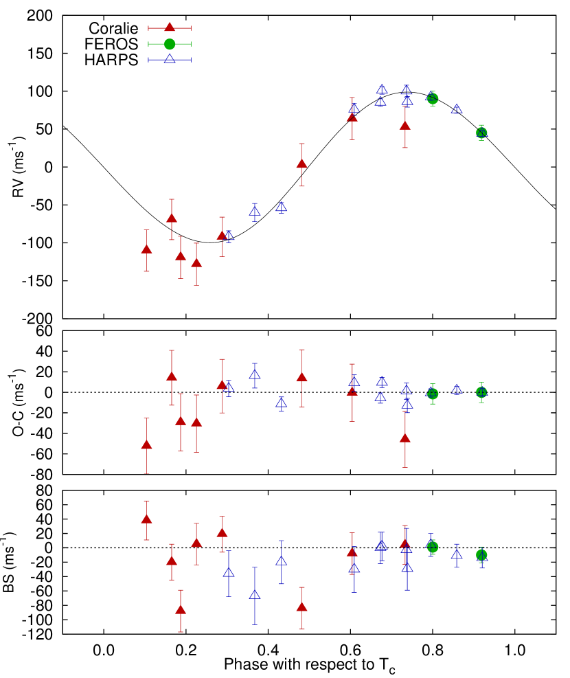
Figure 3.— Top panel: High-precision RV measurements from the MPG 2.2 m/FEROS, the ESO 1.2 m/CORALIE, and the ESO 3.6 m/HARPS instruments, together with our best-fit orbit model. Zero phase corresponds to the time of mid-transit. The center-of-mass velocity has been subtracted. Second panel: Velocity $O\!-\!C$ residuals from the best-fit model. The error bars for each instrument include the jitter which is varied in the fit. Third panel: Bisector spans (BS). Note the different vertical scales of the panels.

Table 3 Relative radial velocities and bisector span measurements of HATS-17.

BJD	RV	$\sigma_{\rm RV}$	BS	$\sigma_{\rm BS}$	Phase	Instrument
(2 456 000$+$)	($\rm m\,s^{-1}$)	($\rm m\,s^{-1}$)	($\rm m\,s^{-1}$)
$1067.79423$	$75.97$	$8.00$	$-30.0$	$32.0$	$0.609$	HARPS
$1068.83188$	$84.97$	$5.00$	$0.0$	$22.0$	$0.673$	HARPS
$1068.89436$	$100.97$	$5.00$	$2.0$	$20.0$	$0.677$	HARPS
$1069.85983$	$99.97$	$8.00$	$-3.0$	$30.0$	$0.736$	HARPS
$1069.89514$	$85.97$	$7.00$	$-29.0$	$30.0$	$0.738$	HARPS
$1070.82342$	$91.97$	$4.00$	$4.0$	$16.0$	$0.795$	HARPS
$1071.84990$	$74.97$	$4.00$	$-11.0$	$16.0$	$0.859$	HARPS
$1072.85895$	$43.97$	$4.00$	$-14.0$	$14.0$	$0.921$	HARPS
$1075.83710$	$-110.14$	$17.00$	$38.0$	$27.0$	$0.104$	Coralie
$1076.82996$	$-69.14$	$16.00$	$-20.0$	$25.0$	$0.165$	Coralie
$1077.81340$	$-128.14$	$18.00$	$5.0$	$29.0$	$0.226$	Coralie
$1078.82533$	$-92.14$	$15.00$	$19.0$	$25.0$	$0.288$	Coralie
$1109.69531$	$-119.14$	$18.00$	$-88.0$	$29.0$	$0.187$	Coralie
$1111.59481$	$-92.03$	$8.00$	$-36.0$	$32.0$	$0.304$	HARPS
$1112.62535$	$-60.03$	$12.00$	$-67.0$	$40.0$	$0.367$	HARPS
$1113.67401$	$-54.03$	$7.00$	$-20.0$	$30.0$	$0.432$	HARPS
$1119.66549$	$90.12$	$10.00$	$1.0$	$10.0$	$0.800$	FEROS
$1121.59323$	$45.12$	$10.00$	$-10.0$	$11.0$	$0.919$	FEROS
$1179.50706$	$2.86$	$18.00$	$-84.0$	$29.0$	$0.482$	Coralie
$1181.49387$	$63.86$	$18.00$	$-8.0$	$29.0$	$0.604$	Coralie
$1183.58674$	$52.86$	$17.00$	$4.0$	$27.0$	$0.733$	Coralie

3. Analysis

Figure 4.— Comparison between the measured values of $T_{\rm eff\star}$ and $\rho_{\star}$ (from ZASPE applied to the FEROS spectra, and from our modeling of the light curves and RV data, respectively), and the Y² model isochrones from Yi et al. (2001). The best-fit values (dark filled circle), and approximate 1$\sigma$ and 2$\sigma$ confidence ellipsoids are shown. The values from our initial ZASPE iteration are shown with the open triangle. The Y² isochrones are shown for ages of 0.2 Gyr, and 1.0 to 14.0 Gyr in 1 Gyr increments.

We analyzed the photometric and spectroscopic observations of HATS-17 to determine the parameters of the system using the standard procedures developed for HATNet and HATSouth (see Bakos et al., 2010, with modifications described by Hartman et al., 2012).

High-precision stellar atmospheric parameters were measured from the FEROS spectra using the ZASPE code (Brahm et al. 2015, in prep). ZASPE estimates the atmospheric stellar parameters and $v\sin{i}$ from high resolution echelle spectra via a least squares method against a grid of synthetic spectra in the most sensitive zones of the spectra to changes in the atmospheric parameters. ZASPE obtains reliable errors in the parameters, as well as the correlations between them by assuming that the principal source of error is the systematic mismatch between the data and the optimal synthetic spectra. We used a synthetic grid provided by Brahm et al. (2015) and the spectral region considered for the analysis was from 5000Å to 6000Å, which includes a large number of atomic transitions and the pressure sensitive Mg Ib lines. We obtained the following high precision parameters with ZASPE: $T_{\rm eff\star}$=5840$\pm$91 K, $\log{g_{\star}}$=4.36$\pm$0.15 dex, $\rm[Fe/H]$=0.30$\pm$0.05 dex and $v\sin{i}$=3.84$\pm$0.48 km/s.

The resulting $T_{\rm eff\star}$ and $\rm[Fe/H]$ measurements were combined with the stellar density $\rho_{\star}$ determined through our joint light curve and RV curve analysis, to determine the stellar mass, radius, age, luminosity, and other physical parameters, by comparison with the Yonsei-Yale (Y²; Yi et al., 2001) stellar evolution models (see Figure 4). This provided a revised estimate of $\log{g_{\star}}$ which was fixed in a second iteration of ZASPE. Our final adopted stellar parameters are listed in Table 4; the final atmospheric parameters are compatible to the ones obtained in the first ZASPE iteration. We find that the star HATS-17 has a mass of $1.131\pm 0.030$ $M_{\sun}$, a radius of $1.091_{-0.046}^{+0.070}$ $R_{\sun}$, and is at a reddening-corrected distance of $340_{-17}^{+22}$ pc.

We also carried out a joint analysis of the high-precision FEROS, CORALIE and HARPS RVs (fit using an eccentric Keplerian orbit) and the HS, PEST 0.3 m, LCOGT 1 m, and Swope 1 m light curves (fit using a Mandel & Agol, 2002 transit model with fixed quadratic limb darkening coefficients taken from Claret, 2004) to measure the stellar density, as well as the orbital and planetary parameters. This analysis makes use of a differential evolution Markov Chain Monte Carlo procedure (DEMCMC; ter Braak, 2006) to estimate the posterior parameter distributions, which we use to determine the median parameter values and their 1$\sigma$ uncertainties. The results are listed in Table 5. We find that the planet HATS-17b has a mass of $1.338\pm 0.065$ $M_{\rm J}$, and a radius of $0.777\pm 0.056$ $R_{\rm J}$. We also find that the observations are consistent with a circular orbit: $e=0.029\pm 0.022$, with a 95% confidence upper-limit of $e<0.070{}$. Note, however, that due to the relatively long orbital period, and thus weak tidal interaction between the planet and star, we do not fix the eccentricity to zero in the fit, as we often do for shorter period planets where there is a prior expectation of the orbit being circular. The uncertainty in the eccentricity thus contributes to the uncertainties of other parameters listed in Table 5.

In order to rule out the possibility that HATS-17 is a blended stellar eclipsing binary system, we carried out a blend analysis of the photometric data following Hartman et al. (2012). We find that all of the blend models considered provide a fit to the photometric data that has a higher $\chi^{2}$ than the model consisting of a single star with a transiting planet, and that the best-fitting blended eclipsing binary model can be rejected with $3\sigma$ confidence in favor of the single star with a planet model. Moreover, the blend models which come closest to fitting the photometry would have easily been detected as a composite system based on the spectroscopic observations (RV and BS variations of several $\rm km\,s^{-1}$). As is often the case, we find that while blends involving stellar eclipsing binaries may be ruled out by the photometry, we cannot exclude the possibility that HATS-17 is a transiting planet system diluted by light from an unresolved stellar companion. We find that including a physical wide binary companion with a mass $M>0.5$ $M_{\sun}$ leads to a slightly higher $\chi^{2}$, but all companions, up to the mass of HATS-17, are permitted within $1\sigma$. If HATS-17 has an unresolved stellar companion, the radius of HATS-17b could be as much as 1.6 times larger than what we infer here (for the extreme case of a star of equal mass to HATS-17).

Our analysis showed that HATS-17 is a relatively young ($\sim$2 Gyr) G-type star with physical parameters very similar to the Sun, but with a substantial metal enrichment ([Fe/H]=$+0.3$). On the other hand, HATS-17b is a weakly irradiated ($T_{\rm eq}\sim$800 K, $\langle F\rangle\sim$10⁸ erg s^-1cm^-2) Jovian planet and due to its relatively long semi-major axis of $\sim$0.13 AU can be classified as a warm Jupiter. One of the principal peculiarities of HATS-17b is that it has a very compact radius for its Jupiter-like mass, yielding a very high density of $\rho_{p}$=3.5 gcm^-3 compared to Jupiter ($\rho_{\rm J}$=1.33 gcm^-3) .

Table 4 Stellar Parameters for HATS-17

Parameter	Value	Source
Identifying Information
R.A. (h:m:s)	$12^{\mathrm{h}}48^{\mathrm{m}}45.72{\mathrm{s}}$	2MASS
Dec. (d:m:s)	$-47{\arcdeg}36{\arcmin}49.3{\arcsec}$	2MASS
R.A.p.m. (mas/yr)	$-32.40\pm 0.90$	2MASS
Dec.p.m. (mas/yr)	$7.5\pm 1.4$	2MASS
GSC ID	GSC 8249-00170	GSC
2MASS ID	2MASS 12484555-4736492	2MASS
Spectroscopic properties
$T_{\rm eff\star}$ (K)	$5846\pm 78$	ZASPE
Spectral type	G	ZASPE
$\rm[Fe/H]$	$0.300\pm 0.030$	ZASPE
$v\sin{i}$ ($\rm km\,s^{-1}$)	$3.73\pm 0.39$	ZASPE
$\gamma_{\rm RV}$ ($\rm m\,s^{-1}$)	$22943.2\pm 4.0$	FEROS
Photometric properties
$B$ (mag)	$13.105\pm 0.090$	APASS
$V$ (mag)	$12.39\pm 0.10$	APASS
$g$ (mag)	$12.665\pm 0.050$	APASS
$r$ (mag)	$12.162\pm 0.060$	APASS
$i$ (mag)	$12.08\pm 0.19$	APASS
$J$ (mag)	$11.082\pm 0.023$	2MASS
$H$ (mag)	$10.837\pm 0.022$	2MASS
$K_{s}$ (mag)	$10.698\pm 0.021$	2MASS
Derived properties
$M_{\star}$ ($M_{\sun}$)	$1.131\pm 0.030$	Y2+$\rho_{\star}$+ZASPE
$R_{\star}$ ($R_{\sun}$)	$1.091_{-0.046}^{+0.070}$	Y2+$\rho_{\star}$+ZASPE
$\log{g_{\star}}$ (cgs)	$4.416\pm 0.042$	Y2+$\rho_{\star}$+ZASPE
$\rho_{\star}$ ($\rm g\,cm^{-3}$)	$1.38\pm 0.27$	Light Curves
$\rho_{\star}$ ($\rm g\,cm^{-3}$)	$1.22\pm 0.17$	$Y^{2}$+Light Curves
$L_{\star}$ ($L_{\sun}$)	$1.24\pm 0.17$	Y2+$\rho_{\star}$+ZASPE
$M_{V}$ (mag)	$4.57\pm 0.15$	Y2+$\rho_{\star}$+ZASPE
$M_{K}$ (mag,ESO)	$3.08\pm 0.12$	Y2+$\rho_{\star}$+ZASPE
Age (Gyr)	$2.1\pm 1.3$	Y2+$\rho_{\star}$+ZASPE
$A_{V}$ (mag)	$0.17\pm 0.11$	Y2+$\rho_{\star}$+ZASPE
Distance (pc)	$339_{-16}^{+22}$	Y2+$\rho_{\star}$+ZASPE

Table 5Parameters for the transiting planet HATS-17b.

Parameter	Value
Light curve parameters
$P$ (days)	$16.254611\pm 0.000073{}$
$T_{c}$ (${\rm BJD}$)	$2457139.1672\pm 0.0014{}$
$T_{14}$ (days)	$0.2011\pm 0.0038{}$
$T_{12}=T_{34}$ (days)	$0.0166\pm 0.0020{}$
$a/R_{\star}$	$25.8_{-1.5}^{+1.1}{}$
$\zeta/R_{\star}$	$10.83\pm 0.20{}$
$R_{p}/R_{\star}$	$0.0726\pm 0.0026{}$
$b^{2}$	$0.187_{-0.083}^{+0.074}{}$
$b\equiv a\cos i/R_{\star}$	$0.432_{-0.110}^{+0.079}{}$
$i$ (deg)	$89.08\pm 0.26{}$
Limb-darkening coefficients
$c_{1},i$ (linear term)	$0.2710{}$
$c_{2},i$ (quadratic term)	$0.3370{}$
$c_{1},r$	$0.3640{}$
$c_{2},r$	$0.3272{}$
RV parameters
$K$ ($\rm m\,s^{-1}$)	$99.1\pm 4.4{}$00
$e$	$0.029\pm 0.022{}$
$\sqrt{e}\cos\omega$	$-0.037\pm 0.087{}$
$\sqrt{e}\sin\omega$	$-0.10_{-0.12}^{+0.16}{}$
Coralie RV jitter ($\rm m\,s^{-1}$)	$6\pm 13$
FEROS RV jitter ($\rm m\,s^{-1}$)	$0.1\pm 9.3$
HARPS RV jitter ($\rm m\,s^{-1}$)	$0.9\pm 4.1$
Planetary parameters
$M_{p}$ ($M_{\rm J}$)	$1.338\pm 0.065{}$
$R_{p}$ ($R_{\rm J}$)	$0.777\pm 0.056{}$
$C(M_{p},R_{p})$	$0.25{}$
$\rho_{p}$ ($\rm g\,cm^{-3}$)	$3.50_{-0.51}^{+0.85}{}$
$\log g_{p}$ (cgs)	$3.737_{-0.044}^{+0.060}{}$
$a$ (AU)	$0.1308\pm 0.0012{}$
$T_{\rm eq}$ (K)	$814\pm 25{}$
$\Theta$	$0.398\pm 0.031{}$
$\langle F\rangle$ ($10^{7}$$\rm erg\,s^{-1}\,cm^{-2}$)	$9.9\pm 1.3{}$

4. Discussion

In this paper we have presented the discovery of HATS-17b, the first transiting warm Jupiter of the HATSouth survey and the transiting extrasolar planet with the longest orbital period detected to date by a ground-based photometric survey. The left panel of Figure 5 shows that HATS-17b, with its period of 16.25 days, lies in a sparsely populated region of the parameter space of confirmed transiting extrasolar giant planets ($M_{p}>0.25\,M_{J}$, $R_{p}>0.5\,R_{J}$) that have measured masses and densities. There are only 19 confirmed giant planets with longer orbital periods, with most of them (17) discovered by the space-based missions Kepler and CoRoT, and orbiting stars that are generally too faint for performing detailed follow-up observations to further characterize those systems. In fact, the masses of ten of the long period planets discovered from space were determined by transit timing variations (TTVs) because it was easier than obtaining precise RV measurements of their faint host stars. HATS-17b, on the other hand, has a bright ($V=12.4$) host which allowed a detailed determination of the orbital parameters of the system via RV measurements and can be the target of future spectroscopic and photometric follow-up.

Due to its relatively large semi-major axis ($a\approx 0.13$ AU), HATS-17b is a low irradiated planet. The flux received per unit area by the planet is $\langle F\rangle$=9.9$\times$10⁷erg cm^-2s^-1, which is low enough that we do not expect heating from the star to significantly impact the structure of the planet (Kovács et al., 2010; Demory & Seager, 2011). The right panel of Figure 5 shows that there are $\sim$30 other well characterized giant planets with $\langle F\rangle$$<$2.0$\times$10⁸erg cm^-2s^-1 that belong to the mentioned group, with 11 of them discovered by ground-based transit surveys orbiting stars at shorter semi-major axes than HATS-17b but around less luminous host stars than HATS-17. In addition to the low insolation level of HATS-17b, the low eccentricity of its orbit ensures that tidal interactions with the star are not able to generate internal heating on the planet. This particular state of HATS-17b is not applicable for the whole group of low irradiated planets as many of them have measurable eccentricities that could generate tidal heating during periastron passages.

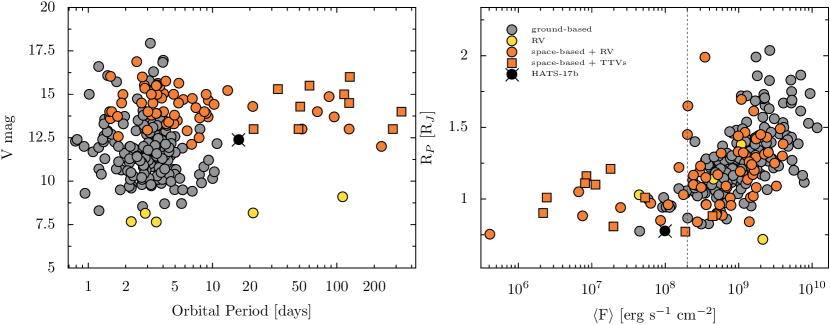
Figure 5.— Left panel: V magnitude of the discovered transiting giant planets ($M_{P}$$>$0.25$M_{J}$, $R_{P}$$>$0.25$R_{J}$) as function of their orbital periods. TEPs discovered by ground-based transit surveys correspond to the gray circles, while RV discovered transiting planets a shown in yellow circles. TEPs discovered from space are shown in orange. Circles correspond to the planets for which the masses determination were performed via RV measurements while squares are used to identify systems for which the masses were estimates with TTVs. The black circle with a cross shows the position of HATS-17b which lies in a sparsely populated region of the parameter space and stands out as the TEP with the longest orbital period discovered to date by a ground-based transit surveys. Right panel: Radii of TEPs as function of the incoming flux per unit area in the surface of the planet. The symbols and colours represent the same features as in the left panel. The vertical dashed line marks the insolation level below which extra heating mechanisms do not produce inflated giant planets. HATS-17b lies in the zone of weakly irradiated planets.

Transiting systems like HATS-17b, in which we can isolate the planetary physical properties from significant heating mechanisms produced by the stellar host, are very important for constraining theoretical models of the structure of giant planets. In Figure 6, the physical properties of HATS-17b are contrasted with the ones of the rest of the well characterized transiting giant exoplanets. Both panels illustrate that HATS-17b is a peculiar object regarding its structure. HATS-17b possesses a radius of $R_{P}$=0.777$R_{\rm J}$ which is extremely compact even for low irradiated planets. The planet that most closely resembles HATS-17b is WASP-59b (Hébrard et al., 2013) with $R_{P}$=0.78$R_{\rm J}$, $M_{P}$=0.86$M_{\rm J}$ and $\langle F\rangle$=4.5$\times$10⁷erg cm^-2s^-1. The rest of the planets that share a similar radius have masses smaller than 0.4$M_{\rm J}$. The compact nature of HATS-17b  is further illustrated in the right panel of Figure 6, where it stands out as the densest giant planet with masses $M_{P}$$<$2$M_{\rm J}$.

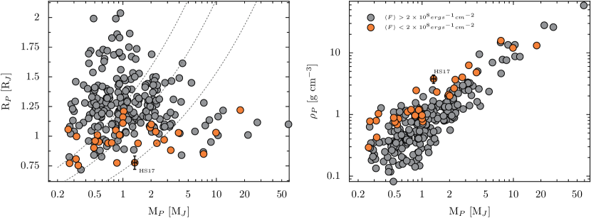
Figure 6.— Left panel: mass-radius diagram of the detected giant TEPs. Black circles are planets with insulation levels greater than $\langle F\rangle<2.0\times 10^{8}$ erg cm^-2s^-1, while orange circles correspond to planets receiving low irradiation. HATS-17b present one of the smallest radii among transiting giant planets. Right panel: density of giant planets as function of the planetary mass. HATS-17b lies at the upper envelope of this distribution.

The small radius of HATS-17b is in concordance with the low irradiation levels of warm Jupiters. However, its particular value is not straight-forward to explain with standard theoretical models of planetary structure. Figure 7 shows that, for the stellar and planetary properties of the HATS-17 system, the Fortney et al. (2007) models for giant planets predict a radius that is more than 3$\sigma$ larger than the observed one even for the maximum available core mass of 100$M_{\earth}$. By performing an extrapolation of the these models we have estimated that a central core of $\sim$200$M_{\earth}$ is required to explain the compact nature of HATS-17b. Such a massive core implies that $\sim$50% of the planet mass is composed of heavy elements, which strongly contrasts with the $\sim$10% we can infer from Jupiter given a $\sim$15$M_{\earth}$ core (Militzer et al., 2008) and is closer to the fraction of heavy elements predicted for the solar system ice giants.

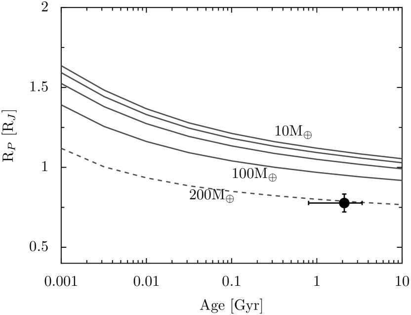
Figure 7.— Evolution models of the radius of a planet as a function of age for the planetary and stellar properties of the HATS-17 system. The solid lines represent models with central core masses of 10, 25, 50 and 100$M_{\earth}$ from Fortney et al. (2007). The dashed line corresponds to an extrapolation of the models for a core mass of 200$M_{\earth}$. The filled circle corresponds to HATS-17b. A very high content of solid material is required to explain the compact radius of HATS-17b.

The massive core inferred for HATS-17b can be linked to the high metallicity of the parent star ([Fe/H]=$+0.3$ dex). In the context of the core accretion scenario of giant planets formation, a more metal rich disk can be more efficient in forming massive cores. Several works (Guillot et al., 2006; Burrows et al., 2007; Miller & Fortney, 2011) have claimed to find a correlation between the stellar metallicity and the amount of heavy elements inferred for giant TEPs. In particular, Miller & Fortney (2011) (hereafter M11) find that for low irradiated planets there is a minimum core mass of $\sim$10$M_{\earth}$ and that from this value the amount of heavy elements present in the planets’ interior raises as a function of [Fe/H], with CoRoT-10b (Bonomo et al., 2010) being the most extreme case with a heavy element content of $M_{c}$=182$\pm$94$M_{\earth}$ and [Fe/H]=$+0.26$ dex. The left panel of Figure 8 shows this claimed correlation for the 14 systems analyzed by M11 and adding HATS-17b. HATS-17b seems to agree quite well with the correlation proposed by M11. Even though the predicted heavy element content for a metallicity of [Fe/H]=$+0.3$ dex should be closer to $\sim$100$M_{\earth}$, the dispersion of the correlation is greater than the individual errors. Clearly, detections of more warm giant TEPs are required.

M11 also proposed a negative correlation between the metal enrichment of the planet relative to the star and the mass of the planet. This correlation is observed in the giant planets of our solar system where Uranus and Neptune are more enriched in heavy elements than Saturn and in turn Saturn is more metal enriched than Jupiter. The right panel of Figure 8 shows that HATS-17b seems to subtly depart from this correlation having enrichments similar to Saturn mass planets rather than the ones of Jupiter mass planets.

Figure 8.— Left: Correlation between the mass of the heavy elements in weakly irradiated planets and the metallicity of the host star. The gray circles correspond to the values found by Miller & Fortney (2011) and the orange circle represents HATS-17. The massive core of HATS-17b can be related to the high metallicity of its host. Right: Negative correlation proposed by Miller & Fortney (2011) between the metal enrichment of the planets with respect to the metal enrichment of the star as a function of the mass of the planet. In this case HATS-17b tends to depart of the correlation and seems to lack of a massive H/He envelope for its given mass.

In summary, the massive core of HATS-17b can be expected given the high metallicity of the parent star, but it seems to lack a more extended H/He envelope. The mechanism that allows the formation of such massive embryos is unclear. If HATS-17b was formed by core accretion at $a=5$ AU and we assume that the total heavy element composition of HATS-17 scales with the iron abundance, we can infer an embryo of $M_{c}$=30$M_{\earth}$, which corresponds to just 15% of the estimated mass of the core of HATS-17b. More massive cores can be formed at larger distances but even if the primordial material is available, the planetesimal accretion rate must exceed the gas accretion rate which should be difficult to accomplish for cores with $M_{c}>$20$M_{\earth}$. An alternative explanation for the extremely massive core of HATS-17b can be related to collisions with other objects in the system posterior to the dispersal of the protoplanetary disk. Liu et al. (2015) proposed, based on numerical simulations, that giant impacts of super-Earth-like planets or mergers with other gas giants generally leads to a total coalescence of impinging gas giants and that sometimes the collisions can disintegrate the envelope of gas giants which may also explain the seeming lack of a massive H/He envelope for HATS-17b. This hypothesis is further supported by the study of Petrovich et al. (2014) which determined that at small semi-major axes ($a<0.5$ AU), gravitational interactions between planets in unstable systems mostly lead to collisions rather than excitation of highly eccentric and inclined planetary orbits.

A more detailed modelling of the structure of HATS-17b, in which the solid material is distributed through the entire envelope of the planet and not only in a central core, can also lower the amount of heavy elements required to explain its small radius. For example, in the case of the massive planet CoRoT-20b (Deleuil et al., 2012, $M_{P}=4.24M_{\rm J}$), the inclusion of the Baraffe et al. (2008) calculations can decrease by a factor of three the 800$M_{\earth}$ in heavy elements that were initially estimated for this planet.

The current orbital distance of HATS-17b from its host star is compatible with migration via angular momentum exchange with the protoplanetary disk. Migrations through gravitational interactions with other planetary and/or stellar companions should excite the eccentricity of the system and then tidal interactions with the star during periastron passages would be responsible of decreasing the semi-major axis and circularising the orbit. The eccentricity of HATS-17b is consistent with $e=0$, while being too far away from it parent star to have suffered from significant tidal interactions. On the other hand, disc migration is expected to suppress any initial eccentricity of giant planets (Dunhill, 2015). While disk migration stands up as the most probable origin for the current semi-major axis of HATS-17b, high eccentricity migration mechanisms cannot be totally discarded. Kozai-Lindov oscillations (Kozai, 1962) produced by interactions with a distant stellar companion (Takeda & Rasio, 2005) or with a closer planetary companion (Naoz et al., 2011) can be taking place but we may be just observing a stage of low eccentricity in the cycle. Long term RV monitoring of HATS-17b can unveil the presence of another object in the system and measurements of the Rossiter-Mclaughlin effect can detect inclinations in the orbit of HATS-17b produced by the interaction with the companion. However, Dong et al. (2014) predicts that non-eccentric warm Jupiters probably present well aligned orbits with the spin of the star.

As evident from the previous paragraphs, HATS-17b belongs to a group of exoplanets that are useful for constraining theories of structure and evolution of giant planets, but which has a low number of well characterized systems discovered to date. The detection of these transiting warm Jupiters around bright stars is fraught with several difficulties due to the low transit probability of long period planets, low occurrence rate of giant planets with respect to terrestrial planets, and the limited duty cycle that one site ground-based transit surveys are affected by. Moreover the confirmation of the planetary nature of transiting warm Jupiter candidates requires extensive spectroscopic and photometric follow-up campaigns in which observations must be spread over many more epochs compared to the follow-up observations required to confirm short period planets. Taking advantage of its three observing sites in the southern hemisphere, separated by almost 120 deg in longitude each, the HATSouth survey can better tackle these difficulties, and HATS-17b is a testament to its capabilities.

Acknowledgements

Development of the HATSouth project was funded by NSF MRI grant NSF/AST-0723074, operations have been supported by NASA grants NNX09AB29G and NNX12AH91H, and follow-up observations received partial support from grant NSF/AST-1108686. R.B. and N.E. are supported by CONICYT-PCHA/Doctorado Nacional. A.J. acknowledges support from FONDECYT project 1130857, BASAL CATA PFB-06, and from the Ministry of Economy, Development, and Tourism’s Millennium Science Initiative through grant IC120009, awarded to The Millennium Institute of Astrophysics, MAS. R.B. and N.E. acknowledge additional support rom the Ministry of Economy, Development, and Tourism’s Millennium Science Initiative through grant IC120009, awarded to The Millennium Institute of Astrophysics, MAS. V.S. acknowledges support form BASAL CATA PFB-06. This work is based on observations made with ESO Telescopes at the La Silla Observatory. This paper also uses observations obtained with facilities of the Las Cumbres Observatory Global Telescope. Work at the Australian National University is supported by ARC Laureate Fellowship Grant FL0992131. We acknowledge the use of the AAVSO Photometric All-Sky Survey (APASS), funded by the Robert Martin Ayers Sciences Fund, and the SIMBAD database, operated at CDS, Strasbourg, France. Operations at the MPG 2.2 m Telescope are jointly performed by the Max Planck Gesellschaft and the European Southern Observatory. The imaging system GROND has been built by the high-energy group of MPE in collaboration with the LSW Tautenburg and ESO. G. B. wishes to thank the warm hospitality of Adéle and Joachim Cranz at the farm Isabis, supporting the operations and service missions of HATSouth.

References

- Bakos et al. (2004) Bakos, G., Noyes, R. W., Kovács, G., et al. 2004, PASP, 116, 266
- Bakos et al. (2010) Bakos, G. Á., Torres, G., Pál, A., et al. 2010, ApJ, 710, 1724
- Bakos et al. (2013) Bakos, G. Á., Csubry, Z., Penev, K., et al. 2013, PASP, 125, 154
- Bakos et al. (2015) Bakos, G. Á., Penev, K., Bayliss, D., et al. 2015, ArXiv e-prints, 1507.01024
- Baraffe et al. (2008) Baraffe, I., Chabrier, G., & Barman, T. 2008, A&A, 482, 315
- Bayliss et al. (2013) Bayliss, D., Zhou, G., Penev, K., et al. 2013, AJ, 146, 113
- Bayliss et al. (2015) Bayliss, D., Hartman, J. D., Bakos, G. Á., et al. 2015, AJ, 150, 49
- Bonomo et al. (2010) Bonomo, A. S., Santerne, A., Alonso, R., et al. 2010, A&A, 520, A65
- Burrows et al. (2007) Burrows, A., Hubeny, I., Budaj, J., & Hubbard, W. B. 2007, ApJ, 661, 502
- Cardelli et al. (1989) Cardelli, J. A., Clayton, G. C., & Mathis, J. S. 1989, ApJ, 345, 245
- Claret (2004) Claret, A. 2004, A&A, 428, 1001
- Dawson (2014) Dawson, R. I. 2014, ApJ, 790, L31
- Deleuil et al. (2012) Deleuil, M., Bonomo, A. S., Ferraz-Mello, S., et al. 2012, A&A, 538, A145
- Demory & Seager (2011) Demory, B.-O., & Seager, S. 2011, ApJS, 197, 12
- Dong et al. (2014) Dong, S., Katz, B., & Socrates, A. 2014, ApJ, 781, L5
- Dopita et al. (2007) Dopita, M., Hart, J., McGregor, P., et al. 2007, Ap&SS, 310, 255
- Dunhill (2015) Dunhill, A. C. 2015, MNRAS, 448, L67
- Fabrycky & Tremaine (2007) Fabrycky, D., & Tremaine, S. 2007, ApJ, 669, 1298
- Fischer et al. (2007) Fischer, D. A., Vogt, S. S., Marcy, G. W., et al. 2007, ApJ, 669, 1336
- Fortney et al. (2007) Fortney, J. J., Marley, M. S., & Barnes, J. W. 2007, ApJ, 659, 1661
- Goldreich & Tremaine (1980) Goldreich, P., & Tremaine, S. 1980, ApJ, 241, 425
- Guillot et al. (2006) Guillot, T., Santos, N. C., Pont, F., et al. 2006, A&A, 453, L21
- Hansen & Barman (2007) Hansen, B. M. S., & Barman, T. 2007, ApJ, 671, 861
- Hartman et al. (2011) Hartman, J. D., Bakos, G. Á., Torres, G., et al. 2011, ApJ, 742, 59
- Hartman et al. (2012) Hartman, J. D., Bakos, G. Á., Béky, B., et al. 2012, AJ, 144, 139
- Hartman et al. (2015) Hartman, J. D., Bayliss, D., Brahm, R., et al. 2015, AJ, 149, 166
- Hébrard et al. (2008) Hébrard, G., Bouchy, F., Pont, F., et al. 2008, A&A, 488, 763
- Hébrard et al. (2013) Hébrard, G., Collier Cameron, A., Brown, D. J. A., et al. 2013, A&A, 549, A134
- Jordán et al. (2014) Jordán, A., Brahm, R., Bakos, G. Á., et al. 2014, AJ, 148, 29
- Kaufer & Pasquini (1998) Kaufer, A., & Pasquini, L. 1998, in Society of Photo-Optical Instrumentation Engineers (SPIE) Conference Series, Vol. 3355, Optical Astronomical Instrumentation, ed. S. D’Odorico, 844–854
- Kovács et al. (2005) Kovács, G., Bakos, G., & Noyes, R. W. 2005, MNRAS, 356, 557
- Kovács et al. (2002) Kovács, G., Zucker, S., & Mazeh, T. 2002, A&A, 391, 369
- Kovács et al. (2010) Kovács, G., Bakos, G. Á., Hartman, J. D., et al. 2010, ApJ, 724, 866
- Kozai (1962) Kozai, Y. 1962, AJ, 67, 591
- Liu et al. (2015) Liu, S.-F., Agnor, C. B., Lin, D. N. C., & Li, S.-L. 2015, MNRAS, 446, 1685
- Mandel & Agol (2002) Mandel, K., & Agol, E. 2002, ApJ, 580, L171
- McLaughlin (1924) McLaughlin, D. B. 1924, ApJ, 60, 22
- Militzer et al. (2008) Militzer, B., Hubbard, W. B., Vorberger, J., Tamblyn, I., & Bonev, S. A. 2008, ApJ, 688, L45
- Miller & Fortney (2011) Miller, N., & Fortney, J. J. 2011, ApJ, 736, L29
- Naef et al. (2001) Naef, D., Latham, D. W., Mayor, M., et al. 2001, A&A, 375, L27
- Naoz et al. (2011) Naoz, S., Farr, W. M., Lithwick, Y., Rasio, F. A., & Teyssandier, J. 2011, Nature, 473, 187
- Penev et al. (2013) Penev, K., Bakos, G. Á., Bayliss, D., et al. 2013, AJ, 145, 5
- Petrovich (2015) Petrovich, C. 2015, ApJ, 805, 75
- Petrovich et al. (2014) Petrovich, C., Tremaine, S., & Rafikov, R. 2014, ApJ, 786, 101
- Queloz et al. (2001) Queloz, D., Mayor, M., Udry, S., et al. 2001, The Messenger, 105, 1
- Queloz et al. (2010) Queloz, D., Anderson, D. R., Collier Cameron, A., et al. 2010, A&A, 517, L1
- Rafikov (2006) Rafikov, R. R. 2006, ApJ, 648, 666
- Rasio & Ford (1996) Rasio, F. A., & Ford, E. B. 1996, Science, 274, 954
- Rossiter (1924) Rossiter, R. A. 1924, ApJ, 60, 15
- Spiegel & Burrows (2013) Spiegel, D. S., & Burrows, A. 2013, ApJ, 772, 76
- Takeda & Rasio (2005) Takeda, G., & Rasio, F. A. 2005, ApJ, 627, 1001
- ter Braak (2006) ter Braak, C. J. F. 2006, Statistics and Computing, 16, 239
- Winn et al. (2010) Winn, J. N., Fabrycky, D., Albrecht, S., & Johnson, J. A. 2010, ApJ, 718, L145
- Wu & Lithwick (2011) Wu, Y., & Lithwick, Y. 2011, ApJ, 735, 109
- Yi et al. (2001) Yi, S., Demarque, P., Kim, Y.-C., et al. 2001, ApJS, 136, 417
- Zhou et al. (2014) Zhou, G., Bayliss, D., Hartman, J. D., et al. 2014, MNRAS, 437, 2831