“Refsdal” Meets Popper: Comparing Predictions of the Reappearance of the Multiply Imaged Supernova Behind MACSJ1149.5+2223
Abstract
Supernova “Refsdal,” multiply imaged by cluster MACSJ1149.5+2223, represents a rare opportunity to make a true blind test of model predictions in extragalactic astronomy, on a time scale that is short compared to a human lifetime. In order to take advantage of this event, we produced seven gravitational lens models with five independent methods, based on Hubble Space Telescope (HST) Hubble Frontier Field images, along with extensive spectroscopic follow-up observations by HST, the Very Large and the Keck Telescopes. We compare the model predictions and show that they agree reasonably well with the measured time delays and magnification ratios between the known images, even though these quantities were not used as input. This agreement is encouraging, considering that the models only provide statistical uncertainties, and do not include additional sources of uncertainties such as structure along the line of sight, cosmology, and the mass sheet degeneracy. We then present the model predictions for the other appearances of SN “Refsdal.” A future image will reach its peak in the first half of 2016, while another image appeared between 1994 and 2004. The past image would have been too faint to be detected in existing archival images. The future image should be approximately one third as bright as the brightest known image (i.e., mag at peak and mag six months before peak), and thus detectable in single-orbit HST images. We will find out soon whether our predictions are correct.
Subject headings:
gravitational lensing: strong1. Introduction
In 1964 Sjur Resfdal speculated that a supernova (SN) multiply imaged by a foreground massive galaxy could be used to measure distances and, therefore, the Hubble constant (Ref64). The basic physics behind this phenomenon is very simple. According to Fermat’s principle, in gravitational optics as in standard optics, multiple images form at the stationary points of the excess arrival time (1985A&A...143..413S; B+N86). The excess arrival time is the result of the competition between the geometric time delay and the Sha64 delay. The arrival time thus depends on the apparent position of the image in the sky as well as the gravitational potential. Since the arrival time is measured in seconds, while all the other lensing observables are measured in angles on the sky, their relationship depends on the angular diameter distance . In the simplest case of single-plane lensing, the time delay between two images is proportional to the so-called time-delay distance, , where and represent the deflector and the source, respectively (see, e.g., for definitions 2006glsw.conf.....M; Tre10; Suy++10).
Over the past decades, many authors have highlighted the importance and applications of identifying such events (e.g., 1998MNRAS.296..763K; 2001ApJ...556L..71H; 2002A&A...393...25G; 2003ApJ...592...17B; 2003MNRAS.338L..25O), computed rates and proposed search strategies (1988ApJ...324..786L; 2000MNRAS.319..549S; 2003ApJ...583..584O; O+M10), and identified highly magnified supernovae (Qui++14).
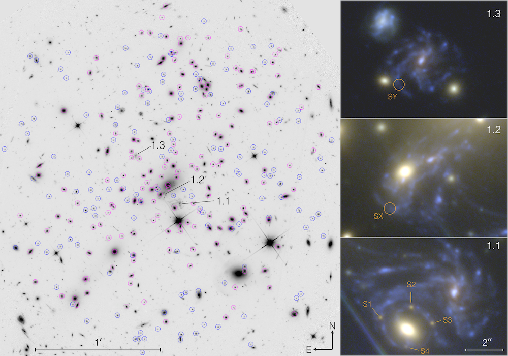
Finally, 50 years after the initial proposal by Refsdal, the first multiply imaged SN was discovered in November 2014 (Kel++15) in Hubble Space Telescope (HST) images of the cluster MACSJ1149.5+2223 (Ebe++07; Smith++09; Zitrin:2009p33878), taken as part of the Grism Lens Amplified Survey from Space (GLASS; GO-13459, PI Treu; Schmidt:2014p33661; Tre++15), and aptly nicknamed “SN Refsdal.” SN Refsdal was identified in difference imaging as four point sources that were not present in earlier images taken as part of the CLASH survey (Postman:2012p27556). Luckily, the event was discovered just before the beginning of an intensive imaging campaign as part of the Hubble Frontier Field (HFF) initiative (Lotz et al. 2015, in prep.; CBZ15). Additional epochs were obtained as part of the Frontier SN program (GO-13790, PI Rodney), and a Director Discretionary Time program (GO/DD-14041, PI Kelly). The beautiful images that have emerged (Figure 1) are an apt celebration of the international year of light and the 100-year anniversary of the theory of general relativity (e.g., T+E15).
The gravitational lensing configuration of SN Refsdal is very remarkable. The SN exploded in one arm of an almost face-on spiral galaxy that is multiply imaged and highly magnified by the cluster gravitational potential ( and ; redshifts from Gri++15). Furthermore, the spiral arm hosting SN Refsdal happens to be sufficiently close to a cluster member galaxy that four additional multiple images are formed with average separation of order arcseconds, typical of galaxy-scale strong lensing. This set of four images close together in an “Einstein cross” configuration is where SN Refsdal has been detected so far (labeled S1–S4 in Fig. 1). As we discuss below, the cluster-scale images are more separated in terms of their arrival time, with time delays that can be much longer than the duration of the event, and therefore it is consistent with the lensing interpretation that they have not yet been seen.
The original suggestion by Ref64 was to use such events to measure distances and therefore cosmological parameters, starting from the Hubble constant. While distances with interesting accuracy and precision have been obtained from gravitational time delays in galaxy-scale systems lensing quasars (e.g., Suy++14), it is premature to attempt this in the case of SN Refsdal. The time delay is not yet known with precision comparable to that attained for lensed quasars (e.g., Tew++13), and the mass distribution of the cluster MACSJ1149.5+2223 is inherently much more complex than that of a single elliptical galaxy.
However, SN Refsdal gives us a unique opportunity to test the current mass models of MACSJ1149.5+2223, by conducting a textbook-like falsifiable experiment (Pop92). All of the models that have been published after the discovery of SN Refsdal (Kel++15; Ogu2015; S+J15; Die++15; Jau++15) predict that an additional image will form some time in the near future (close to image 1.2 of the host galaxy, shown in Figure 1). It could appear as early as October 2015 or in a few years. The field of MACSJ1149.5+2223 is unobservable with HSTat the time of submission of this paper, but observations will resume at the end of October 2015 as part of an approved Cycle 23 program (GO-14199, PI Kelly). We thus have the opportunity to carry out a true blind test of the models, if we act sufficiently fast. This test is similar in spirit to the test of magnification models using singly imaged Type Ia supernovae (Pat+14; Nor+14; Rod++15). The uniqueness of our test lies in the fact that it is based on the prediction of an event that has not yet happened, and it is thus intrinsically blind and immune to experimenter bias.
The quality and quantity of data available to lens modelers have improved significantly since the discovery of SN Refsdal and the publication of the first modeling papers. As part of the HFF and follow-up programs, there are now significantly deeper HST images. Spectroscopy of hundreds of sources in the field (Fig. 1) is available from HST grism data obtained as part of GLASS and SN Refsdal follow-up campaign (PI Kelly), from Multi-Unit Spectroscopic Explorer (MUSE) Very Large Telescope (VLT) Director’s Discretionary Time follow-up observations (Prog. ID 294.A-5032, PI Grillo), and from follow-up observations with the DEep Imaging Multi-Object Spectrograph (DEIMOS Fab++03) on the Keck-II Telescope (PI Jha).
The timing is thus perfect to ask the question: “Given state-of-the-art data and models, how accurately can we predict the arrival time and magnification of the next appearance of a multiply imaged supernova?” Answering this question will give us an absolute measurement of the quality of present-day models, although one should keep in mind that this is a very specific test. The arrival time and especially the magnification of a point source depend strongly on the details of the gravitational potential in the vicinity of the images. Additional uncertainties in the time delay and magnification arise from the inhomogeneous distribution of mass along the line of sight (Suy++10; Collett:2013p34320; Gre++13), the mass-sheet degeneracy and its generalizations (FGS85; SS13; SS14; Suy++14; Xu15), and the residual uncertainties in cosmological parameters, especially the Hubble constant (Rie++11; Fre++12). Average or global quantities of more general interest, such as the total volume behind the cluster, or the average magnification, are much less sensitive to the details of the potential around a specific point.
In order to answer this question in the very short amount of time available, the SN Refsdal follow-up team worked hard to reduce and analyze the new data. By May 2015 it was clear that the quality of the follow-up data would be sufficient to make substantial improvements to their lens models. Therefore, the follow-up team contacted the three other groups who had by then published predictions for SN Refsdal, and offered them the new datasets to update their models, as part of a concerted comparison effort. The five groups worked together to incorporate the new information into the lensing analysis, first by identifying and rigorously vetting new sets of multiple images, and then to promptly update their models to make a timely prediction. A synopsis and comparison between the results and predictions of the various models is presented in this paper. Companion papers by the individual groups will describe the follow-up campaigns as well as the details of each modeling effort.
This paper is organized as follows. In Section 2, we briefly summarize the datasets and measurements that are used in this comparison effort. In Section 3, we review the constraints used by the modeling teams. Section 4 gives a concise description of each of the five lens modeling techniques adopted. Section 5 presents the main results of this paper — a comparison of the predictions of the different models. Section 6 discusses the results, and Section LABEL:sec:summary concludes with a summary. To ensure uniformity with the modeling effort for the Hubble Frontier Fields clusters, we adopt a concordance cosmology with , , and . All magnitudes are given in the AB system (O+G83).
2. Summary of Datasets and Measurements
S2 S1 & 2.11.0 1.090.01 0.81.1 1.130.01 8.0 1.170.01
S3 S1 5.62.2 1.040.02 0.91.1 1.030.01 0.4 1.010.02
S4 S1 2211 0.350.01 14.92.4 0.340.03 30.7 0.380.01
Note. — Observed delays and relative magnifications between images S1–S4 of SN Refsdal. For the values in columns 2 and 3, light curves extending up until July 2015 were used by one of us (P.K.) to derive time delays and magnification ratios using a range of templates. For the values in columns 4 and 5, Rodney et al. (2015, in prep.) matched the observed S1–S4 light curves with the best available SN light-curve template, a model based on SN 1987A with corrections to account for the bluer color of SN Refsdal. The values in columns 6 and 7 were determined by fitting the HST photometry using a second-order Chebyshev polynomial.
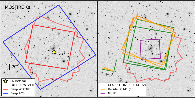
We summarize the datasets and measurements used in this paper. An overview of the field of view and pointing of the instruments used here is shown in Figure 2.
2.1. HST Imaging
Different versions of the images were used at different stages of the process. However, the final identifications of multiple images and their positions were based on the HFF data release v1.0, and their world coordinate system. The reader is referred to the HFF data release webpages111http://www.stsci.edu/hst/campaigns/frontier-fields/ for more information on these data.
2.1.1 The Light Curves of SN Refsdal
Since the discovery of SN Refsdal on November 11, 2014, the MACSJ1149.5+2223 field has been observed in great detail, with HST imaging in optical and infrared bands, and deep spectroscopy from HST, Keck, and the VLT. The main goal of the spectroscopic data is to determine the spectral classification of the SN (Kelly et al. 2015, in prep.). Photometry from the HST imaging provides well-sampled multi-color light curves for SN Refsdal images S1–S4 that exhibit a slow rise over 150 days, reaching a peak brightness in the F160W band on approximately April 13, 2015, with an uncertainty of 20 days in the observer frame (Rodney et al. 2015, in prep.).
The S1–S4 light curves enable a first measurement of the relative time delays and magnification ratios (Rodney et al. 2015, in prep.). Preliminary results from that analysis, using light-curve data up until the end of July 2015, were included in the first version of this paper, which was posted to the arxiv before October 30 in order to make a truly blind prediction before new observations could have revealed the reappearance of SN Refsdal at position SX. Those preliminary time delays were only used as a test of the models and not as an input to the model, so they did not affect any of the predictions given in this paper. Those preliminary measurements obtained by one of us (P.K.) using a range of SN templates are listed in Table 2 for reference. The preliminary peak date of S1 was found to be April 26 2015 ( days), i.e. consistent with the final measurement given here (April 13) within the uncertainties. The final analysis by Rodney et al. (2015) incorporates Cycle 23 observations collected through Nov. 14, 2015. In Section 5.2 we compare our model predictions against all three sets of available measurements of the S1–S4 time delays and magnifications. However, to preserve the blind test, the mass models in this work were not updated to accommodate new information from those late epochs (e.g., the peak is still assumed to be April 26 2015 in the plots).
The Rodney et al. (2015) analysis uses two approaches for the time-delay measurements, first matching the best available SN template (based on SN 1987A) to each of the S1–S4 light curves, and then using a simple polynomial representation for the intrinsic light-curve shape. Uncertainties were derived using a mock light-curve algorithm similar to those developed for lensed quasars (TCM13), although both measurements ignore effects like microlensing fluctuations (doblerkeeton06), and therefore this should be considered as a lower limit to the total uncertainty.
Results from these updated measurements are presented in Table 2 alongside the preliminary ones. The relative magnification ratios are measured to within 2%, and consistent values are derived from both methods. However, the time delays inferred from the two approaches do not agree within the measured uncertainties. This is in part due to the slowly evolving, comparatively featureless light curve of SN Refsdal, and the fact that we were not able observe the MACSJ1149.5+2223 field in August through October, when the SN faded substantially from maximum light. The differences in inferred time delays may also reflect systematic biases inherent to one or both of the measurement methods, as it is possible that none of the available SN light-curve templates or the simple polynomial model are able to accurately represent the intrinsic light-curve shape of this peculiar event. The difference between the two sets of measurements provides an estimate of the systematic uncertainties.
2.2. Spectroscopy
2.2.1 HST Spectroscopy
The HST grism spectroscopy comprises two datasets. The GLASS data consist of 10 orbits of exposures taken through the G102 grism and 4 orbits of exposures taken through the G141 grism, spanning the wavelength range 0.81–1.69 m. The GLASS data were taken at two approximately orthogonal position angles (PAs) to mitigate contamination by nearby sources (the first one on 2014 February 23–25, the second PA on 2014 November 3–11). The SN Refsdal follow-up effort was focused on the G141 grism, reaching a depth of 30 orbits. The pointing and PA of the follow-up grism data were chosen to optimize the spectroscopy of the SN itself, and are therefore different from the ones adopted by GLASS. The SN Refsdal follow-up spectra were taken between 2014 December 23 and 2015 January 4. Only a brief description of the data is given here. For more details the reader is referred to Schmidt:2014p33661 and Tre++15 for GLASS, and Brammer et al. (2015, in prep.) and Kelly et al. (2015, in prep.) for the deeper follow-up data.
The observing strategies and data-reduction schemes were very similar for the two datasets, building on previous work by the 3D-HST survey (Brammer:2012p12977). At least 4 subexposures were taken during each visit with semi-integer pixel offsets. This enables rejection of defects and cosmic rays as well as recovery of some of the resolution lost to undersampling of the point-spread function through interlacing. The data were reduced with an updated version of the 3D-HST reduction pipeline222http://code.google.com/p/threedhst/ described by Brammer:2012p12977 and Mom++15. The pipeline takes care of alignment, defect removal, background removal, image combination, and modeling of contamination by nearby sources. One and two dimensional spectra are extracted for each source.
The spectra were inspected independently by two of us (T.T. and G.B.) using custom tools and the interfaces GiG and GiGz (available at https://github.com/kasperschmidt/GLASSinspectionGUIs) developed as part of the GLASS project. Information obtained from the multiband photometry, continuum, and emission lines was combined to derive a redshift and quality flag. The few discrepancies between redshifts and quality flags were resolved by mutual agreement. In the end, we determined redshifts for 389 sources, with quality 3 or 4 (probable or secure, respectively, as defined by Tre++15).
1 & 177.397188 22.393744 0.0000 4 2
2 177.404017 22.403067 0.5660 4 2
3 177.394525 22.400653 0.5410 4 2
4 177.399663 22.399597 0.5360 4 2
5 177.404054 22.392108 0.0000 4 2
6 177.398554 22.389792 0.5360 4 2
7 177.393010 22.396799 2.9490 4 4 4.1
8 177.394400 22.400761 2.9490 4 2 4.2
9 177.404192 22.406125 2.9490 4 2 4.3
10 177.392904 22.404014 0.5140 4 2
Note. — First entries of the redshift catalog. The full catalog is given in its entirety in the electronic edition. The column “quality” contains the quality flag (3=secure, 4=probable). The column “source” gives the original source of the redshift: 1=HST, Brammer et al. (2015, in prep.); 2=MUSE, (Gri++15); 3=HST+MUSE, 4=MUSE+Keck. The column “note” lists special comments about the object, e.g., if the object is part of a known multiple-image system.
2.2.2 VLT Spectroscopy
Integral-field spectroscopy was obtained with the MUSE instrument on the VLT between 2015 February 14 and 2015 April 12, as part of a Director Discretionary Time program to observe SN Refsdal (PI Grillo). The main goal of the program was to facilitate the computation of an accurate model to forecast the next appearance of the lensed SN. MUSE covers the wavelength range 480–930 nm, with an average spectral resolution of , over a field of view, with a pixel scale of 02 px. Details of the data acquisition and processing are given in a separate paper (Gri++15); only a brief summary of relevant information is given here to guide the reader.
Twelve exposures were collected in dark time under clear conditions and with an average seeing of 10. Bias subtraction, flatfielding, wavelength calibration, and flux calibration were obtained with the MUSE Data Reduction Software version 1.0, as described by Kar++15; Kar2015. The different exposures were combined into a single datacube, with a spectral sampling of 1.25 Å px, and a resulting total integration time of 4.8 hr. One-dimensional (1D) spectra within circular apertures of 06 radius were extracted for all the objects visible in the coadded image along the spectral direction. We also searched in the datacube for faint emission-line galaxies that were not detected in the stacked image. Redshifts were first measured independently by two of the coauthors (W.K. and I.B.) and later reconciled in the very few cases with inconsistent estimates. The analysis yielded secure redshift values for 111 objects, of which 15 are multiple images of 6 different background sources.
2.2.3 Keck Spectroscopy
Spectroscopy of the field was obtained using the DEIMOS spectrograph (Fab++03) on the 10 m Keck-II telescope on 2014 December 20. Conditions were acceptable, with photometric transparency and seeing. The 600 line mm grating was used, set to a central wavelength of 7200 Å, resulting in a scale of 0.65 Å pixel. A multi-slit mask of the field with wide slits was observed for s exposures. The SN images were the main targets, but a slit was also placed on image 4.1, yielding a measurement of its redshift, , independent of but fully consistent with the results from VLT-MUSE. A full analysis of these data and subsequent Keck spectroscopy will be discussed elsewhere.
2.2.4 Combined Redshift Catalog
Redshifts for 70 objects were measured independently using both MUSE and GLASS data. We find that the redshifts of all objects in common agree within the uncertainties, attesting to the excellent quality of the data. The final redshift catalog, consisting of 429 entries, is given in electronic format in Table 2.2.1, and will be available through the GLASS public website at URL https://archive.stsci.edu/prepds/glass/ after the acceptance of this manuscript. We note that owing to the high resolution of the MUSE data, we improved the precision of the redshift of the SN Refsdal host galaxy to (cf. 1.491 previously reported by Smith++09). Also, we revise the redshift of the multiply imaged source 3 with the new and reliable measurement based on unequivocal multiple line identifications ([O II] in the grism data, plus Lyman- in the MUSE data).
3. Summary of Lens Modeling Constraints
3.1. Multiple Images
The strong lensing models that are considered in this paper use as constraints sets of multiply imaged lensed galaxies, as well as knots in the host galaxy of SN Refsdal. The five teams independently evaluated known sets of multiple images (Zitrin:2009p33878; Smith++09; Johnson++14; S+J15; Die++15), and suggested new identifications of images across the entire field of view, based on the new HFF data. In evaluating the image identifications, the teams relied on their preliminary lens models and the newly measured spectroscopic redshifts (Section 2.2). Each team voted on known and new systems on a scale of
| ID | Z09 | S09 | R14, | D15 | Spec- | ref | Spec- | source | Notes | Avg. | Category | ||
|---|---|---|---|---|---|---|---|---|---|---|---|---|---|
| (J2000) | (J2000) | J14 | Score | ||||||||||
| 1.1 | 177.39700 | 22.396000 | 1.2 | A1.1 | 1.1 | 1.1 | 1.4906 | S09 | 1.488 | 3 | 1.0 | Gold | |
| 1.2 | 177.39942 | 22.397439 | 1.3 | A1.2 | 1.2 | 1.2 | 1.4906 | S09 | 1.488 | 3 | 1.0 | Gold | |
| 1.3 | 177.40342 | 22.402439 | 1.1 | A1.3 | 1.3 | 1.3 | 1.4906 | S09 | 1.488 | 3 | 1.0 | Gold | |
| 1.5 | 177.39986 | 22.397133 | 1.4 | 1.5 | 1 | 2.0 | |||||||
| 2.1 | 177.40242 | 22.389750 | 3.3 | A2.1 | 2.1 | 2.3 | 1.894 | S09 | 1.891 | 3 | 1.0 | Gold | |
| 2.2 | 177.40604 | 22.392478 | 3.2 | A2.2 | 2.2 | 2.2 | 1.894 | S09 | 1.891 | 3 | 1.0 | Gold | |
| 2.3 | 177.40658 | 22.392886 | 3.1 | A2.3 | 2.3 | 2.1 | 1.894 | S09 | 1.891 | 3 | 1.0 | Gold | |
| 3.1 | 177.39075 | 22.399847 | 2.1 | A3.1 | 3.1 | 3.1 | 2.497 | S09 | 3.129 | 3 | 2 | 1.0 | Gold |
| 3.2 | 177.39271 | 22.403081 | 2.2 | A3.2 | 3.2 | 3.2 | 2.497 | S09 | 3.129 | 3 | 2 | 1.0 | Gold |
| 3.3 | 177.40129 | 22.407189 | 2.3 | A3.3 | 3.3 | 3.3 | 3.129 | 3 | 2 | 1.1 | Gold | ||
| 4.1 | 177.39300 | 22.396825 | 4.1 | 4.1 | 4.1 | 2.949 | 4 | 1.0 | Gold | ||||
| 4.2 | 177.39438 | 22.400736 | 4.2 | 4.2 | 4.2 | 2.949 | 2 | 1.0 | Gold | ||||
| 4.3 | 177.40417 | 22.406128 | 4.3 | 4.3 | 4.3 | 2.949 | 2 | 1.0 | Gold | ||||
| 5.1 | 177.39975 | 22.393061 | 5.1 | 5.1 | 5.1 | 2.80 | 1 | 1.0 | Gold | ||||
| 5.2 | 177.40108 | 22.393825 | 5.2 | 5.2 | 5.2 | 1.0 | Gold | ||||||
| 5.3 | 177.40792 | 22.403553 | 5.3 | 5.3 | 1.7 | Silver | |||||||
| 6.1 | 177.39971 | 22.392544 | 6.1 | 6.1 | 6.1 | 1.1 | Gold | ||||||
| 6.2 | 177.40183 | 22.393858 | 6.2 | 6.2 | 6.2 | 1.1 | Gold | ||||||
| 6.3 | 177.40804 | 22.402506 | 5.4/6.3 | 6.3 | 1.7 | Silver | |||||||
| 7.1 | 177.39896 | 22.391339 | 7.1 | 7.1 | 1.1 | Gold | |||||||
| 7.2 | 177.40342 | 22.394269 | 7.2 | 7.2 | 1.1 | Gold | |||||||
| 7.3 | 177.40758 | 22.401242 | 7.3 | 1.2 | Gold | ||||||||
| 8.1 | 177.39850 | 22.394350 | 8.1 | 8.1 | 8.1 | 1.2 | Gold | ||||||
| 8.2 | 177.39979 | 22.395044 | 8.2 | 8.2 | 8.2 | 1.2 | Gold | ||||||
| 8.4 | 177.40709 | 22.404722 | 3 | 1.2 | Gold | ||||||||
| 177.40704 | 22.405553 | 2.78 | 1 | 3 | 3.0 | Rejected | |||||||
| 177.40517 | 22.401563 | 8.3 | 3 | 3.0 | Rejected | ||||||||
| 9.1 | 177.40517 | 22.426233 | A6.1 | 9.1 | 1.8 | ||||||||
| 9.2 | 177.40388 | 22.427231 | A6.2 | 9.2 | 1.8 | ||||||||
| 9.3 | 177.40325 | 22.427228 | A6.3 | 9.3 | 1.8 | ||||||||
| 9.4 | 177.40364 | 22.426422 | A6.4? | 1.8 | |||||||||
| 10.1 | 177.40450 | 22.425514 | A7.1 | 10.1 | 1.8 | ||||||||
| 10.2 | 177.40362 | 22.425636 | A7.2 | 10.2 | 1.8 | ||||||||
| 10.3 | 177.40221 | 22.426625 | A7.3 | 10.3 | 1.8 | ||||||||
| 12.1 | 177.39857 | 22.389356 | 1.020 | 3 | 4 | 2.6 | Rejected | ||||||
| 12.2 | 177.40375 | 22.392345 | 0.929 | 2 | 4 | 2.9 | Rejected | ||||||
| 12.3 | 177.40822 | 22.398801 | 1.118 | 3 | 4 | 2.6 | Rejected | ||||||
| 13.1 | 177.40371 | 22.397786 | 13.1 | 1.23 | 1 | 1.0 | Gold | ||||||
| 13.2 | 177.40283 | 22.396656 | 13.2 | 1.25 | 1 | 1.0 | Gold | ||||||
| 13.3 | 177.40004 | 22.393858 | 13.3 | 1.23 | 1 | 1.3 | Gold | ||||||
| 14.1 | 177.39167 | 22.403489 | 14.1 | 3.703 | 2 | 1.3 | Gold | ||||||
| 14.2 | 177.39083 | 22.402647 | 14.2 | 3.703 | 2 | 1.3 | Gold | ||||||
| 110.1 | 177.40014 | 22.390162 | 3.214 | 2 | 1.0 | Gold | |||||||
| 110.2 | 177.40402 | 22.392894 | 3.214 | 2 | 1.0 | Gold | |||||||
| 110.3 | 177.40907 | 22.400242 | 2.0 | ||||||||||
| 21.1 | 177.40451 | 22.386704 | 1.8 | Silver | |||||||||
| 21.2 | 177.40800 | 22.389057 | 1.6 | Silver | |||||||||
| 21.3 | 177.40907 | 22.390407 | 1.6 | Silver | |||||||||
| 22.1 | 177.40370 | 22.386838 | 1.8 | ||||||||||
| 22.2 | 177.40791 | 22.389232 | 1.8 | ||||||||||
| 22.3 | 177.40902 | 22.391053 | 1.8 | ||||||||||
| 23.1 | 177.39302 | 22.411428 | A5 | 1.8 | |||||||||
| 23.2 | 177.39308 | 22.411455 | A5 | 1.8 | |||||||||
| 23.3 | 177.39315 | 22.411473 | A5 | 1.8 | |||||||||
| 24.1 | 177.39285 | 22.412872 | 1.7 | ||||||||||
| 24.2 | 177.39353 | 22.413071 | 1.7 | ||||||||||
| 24.3 | 177.39504 | 22.412697 | 1.8 | ||||||||||
| 25.1 | 177.40428 | 22.398782 | 2.0 | ||||||||||
| 25.2 | 177.40411 | 22.398599 | 2.0 | ||||||||||
| 25.3 | 177.39489 | 22.391796 | 2.3 | ||||||||||
| 26.1 | 177.41035 | 22.388749 | 9.1 | 1.8 | Silver | ||||||||
| 26.2 | 177.40922 | 22.387697 | 9.2 | 1.8 | Silver | ||||||||
| 26.3 | 177.40623 | 22.385369 | 1.8 | Silver | |||||||||
| 27.1 | 177.40971 | 22.387665 | 1.8 | Silver | |||||||||
| 27.2 | 177.40988 | 22.387835 | 1.8 | Silver | |||||||||
| 27.3 | 177.40615 | 22.385142 | 2.5 | ||||||||||
| 28.1 | 177.39531 | 22.391809 | 2.0 | ||||||||||
| 28.2 | 177.40215 | 22.396750 | 2.2 | ||||||||||
| 28.3 | 177.40562 | 22.402434 | 2.0 | ||||||||||
| 200.1 | 177.40875 | 22.394467 | 2.32 | 1 | 2.6 | ||||||||
| 200.2 | 177.40512 | 22.391261 | 2.6 | ||||||||||
| 200.3 | 177.40256 | 22.389233 | 2.8 | ||||||||||
| 201.1 | 177.40048 | 22.395444 | 5 | 1.6 | |||||||||
| 201.2 | 177.40683 | 22.404517 | 5 | 1.6 | |||||||||
| 202.1 | 177.40765 | 22.396789 | 2.0 | ||||||||||
| 202.2 | 177.40224 | 22.391489 | 2.0 | ||||||||||
| 202.3 | 177.40353 | 22.392586 | 2.0 | ||||||||||
| 203.1 | 177.40995 | 22.387244 | 1.8 | Silver | |||||||||
| 203.2 | 177.40657 | 22.384511 | 2.0 | Silver | |||||||||
| 203.3 | 177.41123 | 22.388461 | 1.8 | Silver | |||||||||
| 204.1 | 177.40961 | 22.386661 | 1.8 | Silver | |||||||||
| 204.2 | 177.40668 | 22.384322 | 1.8 | Silver | |||||||||
| 204.3 | 177.41208 | 22.389056 | 1.8 | Silver | |||||||||
| 205.1 | 177.40520 | 22.386042 | 2.0 | ||||||||||
| 205.2 | 177.40821 | 22.388119 | 2.0 | ||||||||||
| 205.3 | 177.41038 | 22.390625 | 2.0 | ||||||||||
| 206.1 | 177.40764 | 22.385647 | 2.2 | ||||||||||
| 206.2 | 177.40863 | 22.386453 | 2.2 | ||||||||||
| 206.3 | 177.41133 | 22.388997 | 2.2 | ||||||||||
| 207.1 | 177.40442 | 22.397303 | 2.2 | ||||||||||
| 207.2 | 177.40397 | 22.396039 | 2.2 | ||||||||||
| 208.1 | 177.40453 | 22.395761 | 2.0 | ||||||||||
| 208.2 | 177.40494 | 22.396397 | 2.0 | ||||||||||
| 209.1 | 177.38994 | 22.412694 | 3.0 | ||||||||||
| 209.2 | 177.39055 | 22.413408 | 3.0 | ||||||||||
| 210.1 | 177.39690 | 22.398061 | 0.702 | 2 | 3.0 | ||||||||
| 210.2 | 177.39505 | 22.397497 | 0.702 | 2 | 3.0 |
Note. — Coordinates and ID notations of multiply imaged families of lensed galaxies. The labels in previous publications are indicated for Zitrin et al. (2009; Z09), Smith et al. (2009; S09), Richard et al. (2014; R14), Johnson et al. (2014; J14), and Diego et al. (2015; D15). New identifications were made by Sharon, Oguri, and Hoag. Each modeling team used a modified version or subset of the list above, with the coordinates of each knot varying slightly between modelers. The source of the new spectroscopic redshift is as in Table 2.2.1: 1=HST, Brammer et al. (2015, in prep.); 2=MUSE, (Gri++15); 3=HST+MUSE; 4=MUSE+Keck. The redshift of image 4.1 was measured independently at Keck (§ 2.2.3). The average score among the team is recorded; “1” denotes secure identification, “2” is a possible identification, and higher scores are considered unreliable by the teams.
See Table 4 for information on all the knots in source 1.
We revise the redshift of source 3 with the new and reliable measurement from MUSE (see § 2.2).
We revise the identification of a counterimage of 8.1 and 8.2, and determine that it is at a different position compared to previous publications. To limit confusion we label the newly identified counterimage 8.4.
The identification of source 12 was ruled out in HFF work prior to the 2014 publications; we further reject this set with spectroscopy.
This image is identified as part of the same source as source 8; the third image is buried in the light of a nearby star.
1–4, where 1 denotes secure identification, 2 is a possible identification, and higher values are considered unreliable. Images that had large variance in their scores were discussed and reevaluated, and the final score was then recorded. The list of multiple images considered in this work is given in Table 3. For each system we give coordinates, the average score, and the redshift if available. We also indicate the labels given to known images that were previously identified in the literature, previously published redshifts, and references to these publications.
We define three samples of image sets (“gold,” “silver,” and “all”) based on the voting process. Following the approach of Wan+15, we conservatively include in our gold sample only the systems about which every team was confident. The silver sample includes images that were considered secure by most teams, or are outside the MUSE field of view. The “all” sample includes all of the images that were not rejected as false identifications, based on imaging and/or spectroscopy. In order to facilitate the comparison, most teams produced baseline models based on the gold sample of images, and some of the teams produced additional models based on larger sets of images. However, owing to differences in investigators’ opinions and specifics of each code, small differences between the constraints adopted by each team persist. They are described below for each of the teams. The reader is referred to the publications of each individual team for more details.
We also evaluated the identification of knots in the spiral galaxy hosting SN Refsdal. Table 4 and Figure 3 list the emission knots and features in the host galaxy of SN Refsdal that were considered in this work. Not all knots were used in all models, and again, there are slight differences between the teams as the implementation of these constraints vary among lensing algorithms. Nevertheless, the overall mapping of morphological features between the images of this galaxy was in agreement between the modeling teams.

3.2. Time Delays
The time delay and magnification ratios between the known images were not yet measured at the time when the models were being finalized. Therefore, they were not used as input and they can be considered as a valuable test of the lens model.
3.3. Cluster Members
Cluster member galaxies were selected based on their redshifts in the combined redshift catalog and their photometry, as follows. In order to account for the cluster velocity dispersion, as well as the uncertainty in the grism-based redshifts, we define cluster membership loosely as galaxies with spectroscopic redshift in the range , within a few thousand kilometers per second of the fiducial cluster redshift (). This is sufficiently precise for the purpose of building lens models, even though not all the cluster members are necessarily physically bound to the cluster, from a dynamical point of view. Naturally, these cluster members still contribute to the deflection field as the dynamically bound cluster members. The spectroscopic cluster-member catalog comprises 170 galaxies.
To obtain a more complete member catalog, the spectroscopically confirmed members were supplemented by photometrically selected galaxies. This list includes galaxies down to the limit (F814W 25 mag) of spectroscopically confirmed members. It consists mostly of galaxies belonging to the last two-magnitude bins of the luminosity distribution, for which the spectroscopic sample is significantly incomplete. The missing galaxies from the spectroscopic catalog are the brightest ones that fall outside the MUSE field of view or the ones that are contaminated in the HST grism data. The photometric analysis is restricted to the WFC3-IR area, in order to exploit the full multi-band photometric catalog from CLASH. The method is briefly described by Gri2015, and it uses a Bayesian technique to compute the probability for a galaxy to be a member from the distribution in color space of all spectroscopic galaxies (from 13 bands — i.e., not including the 3 in the UV). For the photometric selection, we started from spectroscopically confirmed members, with redshift within , and provided a catalog with only the objects having measured F160W magnitudes. The total catalog of cluster members comprises 170 galaxies with spectroscopically determined membership, and 136 galaxies with photometrically determined membership.
| ID | (J2000) | (J2000) | ID Smith et al. (2009) | ID Sharon et al. (2015) | ID Diego et al. (2015) | Notes |
|---|---|---|---|---|---|---|
| 1.1.1 | 177.39702 | 22.396003 | 2 | 1.1 | 1.1.1 | 1 |
| 1.1.2 | 177.39942 | 22.397439 | 2 | 1.2 | 1.2.1 | 1 |
| 1.1.3 | 177.40341 | 22.402444 | 2 | 1.3 | 1.3.1 | 1 |
| 1.*1.5 | 177.39986 | 22.397133 | 1.5.1 | 1,2 | ||
| 1.2.1 | 177.39661 | 22.396308 | 19 | 23.1 | 1.1.8 | |
| 1.2.2 | 177.39899 | 22.397867 | 19 | 23.2 | 1.2.8 | |
| 1.2.3 | 177.40303 | 22.402681 | 19 | 23.3 | 1.3.8 | |
| 1.2.4 | 177.39777 | 22.398789 | 19 | 23.4 | 1.4.8a | |
| 1.2.6 | 177.39867 | 22.398242 | 1.4.8b | |||
| 1.3.1 | 177.39687 | 22.396219 | 16 | 31.1 | 1.1.15 | |
| 1.3.2 | 177.39917 | 22.397600 | 16 | 31.2 | 1.2.15 | |
| 1.3.3 | 177.40328 | 22.402594 | 16 | 31.3 | 1.3.15 | |
| 1.4.1 | 177.39702 | 22.396214 | 11 | 32.1 | ||
| 1.4.2 | 177.39923 | 22.397483 | 11 | 32.2 | ||
| 1.4.3 | 177.40339 | 22.402558 | 11 | 32.3 | ||
| 1.5.1 | 177.39726 | 22.396208 | 18 | 33.1 | ||
| 1.5.2 | 177.39933 | 22.397303 | 18 | 33.2 | ||
| 1.5.3 | 177.40356 | 22.402522 | 18 | 33.3 | ||
| 1.6.1 | 177.39737 | 22.396164 | 1.1.13 | |||
| 1.6.2 | 177.39945 | 22.397236 | 1.2.13 | |||
| 1.6.3 | 177.40360 | 22.402489 | 1.3.13 | |||
| 1.7.1 | 177.39757 | 22.396114 | 40.1 | |||
| 1.7.2 | 177.39974 | 22.396933 | 40.2 | |||
| 1.7.3 | 177.40370 | 22.402406 | 40.3 | |||
| 1.8.1 | 177.39795 | 22.396014 | ||||
| 1.8.2 | 177.39981 | 22.396750 | ||||
| 1.8.3 | 177.40380 | 22.402311 | ||||
| 1.9.1 | 177.39803 | 22.395939 | 1.1.9 | |||
| 1.9.2 | 177.39973 | 22.396983 | 1.2.9 | |||
| 1.9.3 | 177.40377 | 22.402250 | 1.3.9 | |||
| 1.10.1 | 177.39809 | 22.395856 | ||||
| 1.10.2 | 177.39997 | 22.396708 | 36.2 | |||
| 1.10.3 | 177.40380 | 22.402183 | 36.3 | |||
| 1.11.2 | 177.40010 | 22.396661 | 1.2.3 | |||
| 1.11.3 | 177.40377 | 22.402047 | 1.3.3 | |||
| 1.12.1 | 177.39716 | 22.395211 | 1.1.14 | |||
| 1.12.2 | 177.40032 | 22.396925 | 1.2.14 | |||
| 1.12.3 | 177.40360 | 22.401878 | 1.3.14 | |||
| 1.13.1 | 177.39697 | 22.396639 | 7 | 24.1 | 1.1.19 | |
| 1.13.2 | 177.39882 | 22.397711 | 7 | 24.2 | 1.2.19 | |
| 1.13.3 | 177.40329 | 22.402828 | 7 | 24.3 | 1.3.19 | |
| 1.13.4 | 177.39791 | 22.398433 | 7 | 24.4 | 1.4.19 | |
| 1.*13.6 | 177.39852 | 22.398061 | 3 | |||
| 1.14.1 | 177.39712 | 22.396725 | 6 | 25.1 | 1.1.7 | |
| 1.14.2 | 177.39878 | 22.397633 | 6 | 25.2 | 1.2.7 | |
| 1.14.3 | 177.40338 | 22.402872 | 6 | 25.3 | 1.3.7 | |
| 1.14.4 | 177.39810 | 22.398256 | 25.4 | 1.4.7 | ||
| 1.15.1 | 177.39717 | 22.396506 | 41.1 | 1.1.20 | ||
| 1.15.2 | 177.39894 | 22.397514 | 41.2 | 1.2.20 | ||
| 1.15.3 | 177.40344 | 22.402753 | 41.3 | 1.3.20 | ||
| 1.16.1 | 177.39745 | 22.396400 | 4 | 26.1 | 1.1.6 | |
| 1.16.2 | 177.39915 | 22.397228 | 4 | 26.2 | 1.2.6 | |
| 1.16.3 | 177.40360 | 22.402656 | 4 | 26.3 | 1.3.6 | |
| 1.17.1 | 177.39815 | 22.396347 | 3 | 11.1 | 1.1.5 | |
| 1.17.2 | 177.39927 | 22.396831 | 3 | 11.2 | 1.2.5 | |
| 1.17.3 | 177.40384 | 22.402564 | 3 | 11.3 | 1.3.5 | |
| 1.18.1 | 177.39850 | 22.396100 | 1.1.11 | |||
| 1.18.2 | 177.39947 | 22.396592 | 1.2.11 | |||
| 1.18.3 | 177.40394 | 22.402408 | 1.3.11 | |||
| 1.19.1 | 177.39689 | 22.395761 | 21.1 | 1.1.17 | ||
| 1.19.2 | 177.39954 | 22.397486 | 21.2 | 1.2.17 | ||
| 1.19.3 | 177.40337 | 22.402292 | 21.3 | 1.3.17 | ||
| 1.19.5 | 177.39997 | 22.397106 | 21.4 | 1.5.17 | ||
| 1.20.1 | 177.39708 | 22.395728 | 27.1 | 1.1.16 | ||
| 1.20.2 | 177.39963 | 22.397361 | 1.2.16 | |||
| 1.20.3 | 177.40353 | 22.402233 | 27.3 | 1.3.16 | ||
| 1.20.5 | 177.40000 | 22.396981 | 27.2 | 1.5.16 | ||
| 1.21.1 | 177.39694 | 22.395406 | 1.1.18 | |||
| 1.21.3 | 177.40341 | 22.402006 | 1.3.18 | |||
| 1.21.5 | 177.40018 | 22.397042 | 1.5.18 | |||
| 1.22.1 | 177.39677 | 22.395487 | ||||
| 1.22.2 | 177.39968 | 22.397495 | ||||
| 1.22.3 | 177.40328 | 22.402098 | ||||
| 1.22.5 | 177.40008 | 22.397139 | ||||
| 1.23.1 | 177.39672 | 22.395381 | 15 | 22.1 | 1.1.2 | |
| 1.23.2 | 177.39977 | 22.397497 | 15 | 22.2 | 1.2.2 | |
| 1.23.3 | 177.40324 | 22.402011 | 15 | 22.3 | 1.3.2 | |
| 1.23.5 | 177.40013 | 22.397200 | 22.2 | 1.5.2 | ||
| 1.24.1 | 177.39650 | 22.395589 | 28.1 | 1.1.4 | ||
| 1.24.2 | 177.39953 | 22.397753 | 28.2 | 1.2.4 | ||
| 1.24.3 | 177.40301 | 22.402203 | 28.3 | 1.3.4 | ||
| 1.25.1 | 177.39657 | 22.395933 | 1.1.21 | |||
| 1.25.3 | 177.40304 | 22.402456 | 1.3.21 | |||
| 1.27.1 | 177.39831 | 22.396285 | 37.1 | |||
| 1.27.2 | 177.39933 | 22.396725 | 37.2 | |||
| 1.26.1 | 177.39633 | 22.396011 | 1.1.12 | |||
| 1.26.3 | 177.40283 | 22.402600 | 1.3.12 | |||
| 1.28.1 | 177.39860 | 22.396166 | 38.1 | |||
| 1.28.2 | 177.39942 | 22.396559 | 38.2 | |||
| 1.29.1 | 177.39858 | 22.395860 | 39.1 | |||
| 1.29.2 | 177.39976 | 22.396490 | 39.2 | |||
| 1.30.1 | 177.39817 | 22.395465 | 35.1 | |||
| 1.30.2 | 177.39801 | 22.395230 | 35.2 | |||
| 1.30.3 | 177.39730 | 22.395364 | 35.3 | |||
| 1.30.4 | 177.39788 | 22.395721 | 35.4 | |||
| SN1 | 177.39823 | 22.395631 | 30.1 | 1.1.3a | ||
| SN2 | 177.39772 | 22.395783 | 30.2 | 1.1.3b | ||
| SN3 | 177.39737 | 22.395539 | 30.3 | 1.1.3c | ||
| SN4 | 177.39781 | 22.395189 | 30.4 | 1.1.3d |
Note. — Coordinates and ID notations of emission knots in the multiply imaged host of SN Refsdal, at . The labels in previous publications are indicated. New identifications were made by C.G., K.S., and J.D. Each modeling team used a modified version or subset of the list above, with the coordinates of each knot varying slightly between modelers. Nevertheless, there is consensus among the modelers on the identification and mapping of the different features between the multiple images of the same source.
Images 1.1, 1.2, 1.3, and 1.5 were labeled by Zitrin:2009p33878 as 1.2, 1.3, 1.1, and 1.4, respectively. The labels of other knots were not given in that publication.
This knot was identified as a counterimage of the bulge of the galaxy by Zitrin:2009p33878, but rejected by Smith++09. As in the paper by S+J15, the modelers’ consensus is that this knot is likely at least a partial image of the bulge.
Image 1.13.6 is predicted by some models to be a counterimage of 1.13, but its identification is not sufficiently confident to be used as constraint.
4. Brief Description of Modeling Techniques and their Inputs
For convenience to the reader, in this section we give a brief description of each of the modeling techniques compared in this work (summarized briefly in Table 4). We note that the five models span a range of very different assumptions. Three of the teams (Grillo et al., Oguri et al., Sharon et al.) used an approach based on modeling the mass distribution with a set of physically motivated components, described each by a small number of parameters, representing the galaxies in the cluster and the overall cluster halo. We refer to these models as “simply-parametrized.” One of the approaches (Diego et al.) describes the mass distribution with a larger number of components. The components are not associated with any specific physical object and are used as building blocks, allowing for significant flexibility, balanced by regularization. We refer to this model as “free-form”333These models are sometimes described incorrectly as “nonparametric,” even though they typically have more parameters than the so-called parametric models.. The fifth approach (Zitrin et al.) is based on the assumption that light approximately traces mass, and the mass components are built by smoothing and rescaling the observed surface brightness of the cluster members. We refer to this approach as “light-traces-mass.” All of the models considered here are single-plane lens models. As we will discuss in Section 6, each type of model uses a different approach to account for the effects of structure along the line of sight, and to break the mass-sheet degeneracy. All model outputs will be made available through the HFF website after the acceptance of the individual modeling papers.
Die-a & Diego et al. Free-form 0.78 gold+sil
Gri-g Grillo et al. Simply-param 0.26 gold
Ogu-g Oguri et al. Simply-param 0.43 gold
Ogu-a Oguri et al. Simply-param 0.31 all
Sha-g Sharon et al. Simply-param 0.16 gold
Sha-a Sharon et al. Simply-param 0.19 gold+sil
Zit-g Zitrin et al. Light-tr-mass 1.3 gold
Note. — For each model we provide a short name as well as basic features and inputs. The column RMS lists the root-mean-square scatter of the observed vs. predicted image positions in arcseconds.
We note that members of our team have developed another complementary “free-form” approach, based on modeling the potential in pixels on an adaptive grid (Bra++04; Bra++09). However, given the pixelated nature of the reconstruction and the need to compute numerical derivatives and interpolate from noisy pixels in order to compute time delays and magnifications at the location of SN Refsdal, we did not expect this method to be competitive for this specific application. Therefore, in the interest of time we did not construct this model. A pre-HFF model of MACSJ1149.5+2223 using this approach is available through the HFF website and will be updated in the future.
When appropriate, we also describe additional sets of constraints used by each modeler.
4.1. Diego et al.
A full description of the modeling technique used by this team (J.D., T.B.) and the various improvements implemented in the code can be found in the literature (Diego2005; Diego2007; Sendra2014; Die++15). Here is a brief summary of the basic steps.
4.1.1 Definition of the Mass Model
The algorithm (WSLAP+) relies on a division of the mass distribution in the lens plane into two components. The first is compact and associated with the member galaxies (mostly red ellipticals). The second is diffuse and distributed as a superposition of Gaussians on a regular (or adaptive) grid. In this specific case, a grid of pixels on a side was used. For the compact component, the mass associated with the galaxies is assumed to be proportional to their luminosity. If all the galaxies are assumed to have the same mass-to-light () ratio, the compact component (galaxies) contributes with just one () extra free parameter which corresponds to the correction that needs to be applied to the fiducial ratio. In a few particular cases, some galaxies (like the brightest cluster galaxy [BCG] or massive galaxies very close to an arclet) are allowed to have their own ratio, adding additional free parameters to the lens model but typically no more than a few ( O(1)). For this component associated with the galaxies, the total mass is assumed to follow either a NFW97 profile (with a fixed concentration, and scale radius scaling with the fiducial halo mass) or be proportional to the observed surface brightness. For this work the team adopted or . The case considers one central BCG and the elliptical galaxy near image 1.2 to have the same ratio, while the remaining galaxies have a different one. In the case , the BCG and the galaxy near image 1.2 each have their own ratio, and the remaining galaxies are assumed to have a third independent value. In all cases, it is important to emphasize that the member galaxy between the 4 observed images of SN Refsdal was not allowed to have its own independent ratio. This results in a model that is not as accurate on the smallest scales around this galaxy as other models that allow this galaxy to vary.
The diffuse or “soft” component is described by as many free parameters as grid (or cell) points. This number () varies but is typically between a few hundred to one thousand ( O(100)-O(1000)) depending on the resolution and/or use of the adaptive grid. In addition to the free parameters describing the lens model, the problem includes as unknowns the original positions of the lensed galaxies in the source plane. For the clusters included in the HFF program the number of background sources, , is typically a few tens ( O(10)), each contributing with two unknowns ( and ). All of the unknowns are then combined into a single array with elements ().
4.1.2 Definition of the Inputs
The inputs are the pixel position of the strongly lensed galaxies (not just the centroids) for all the multiple images listed in Tables 3 and 4. In the case of elongated arcs near the critical curves with no features, the entire arc is mapped and included as a constraint. If the arclets have individual features, these can be incorporated as semi-independent constraints but with the added condition that they need to form the same source in the source plane. The following inputs are added to the default set of image and knot centers listed in Section 3:
-
1.
Shape of the arclets. This is particularly useful for long elongated arcs (with no counterimages) which lie in the regime between the weak and strong lensing. These arcs are still useful constraints that add valuable information beyond the Einstein radius.
-
2.
Shape and morphology of arcs. By including this information one can account (at least partially) for the magnification at a given position.
-
3.
Resolved features in individual systems. This new addition to the code is motivated by the host galaxy of SN Refsdal, where multiple features can be identified in the different counter images. In addition, the counterimage in the North, when relensed, offers a robust picture of the original source morphology (size, shape, orientation). This information acts as an anchor, constraining the range of possible solutions.
Weak lensing shear measurements can also be used as input to the inference. For the particular case of MACSJ1149.5+2223 the weak lensing measurements are not used, to ensure homogeneity with the other methods.
4.1.3 Description of the Inference Process and Error Estimation
The array of best-fit parameters, , is obtained after solving the system of linear equations
| (1) |
where the observations (strong lensing, weak lensing, time delays) are included in the array , and the matrix is known and has dimension .
In practice, is obtained by solving the set of linear equations described in Eq. 1 via a fast biconjugate algorithm, or inverted with a singular value decomposition (after setting a threshold for the eigenvalues) or solved with a more robust but slower quadratic algorithm. The quadratic algorithm is the preferred method, as it imposes the physical constraint that the solution must be positive. This eliminates unphysical solutions with negative masses and reduces the space of possible solutions. Like in the case of the biconjugate gradient, the quadratic programming algorithm solves the system of linear equations by finding the minimum of the associated quadratic function. Errors in the solution are derived by minimizing the quadratic function multiple times, after varying the initial conditions of the minimization process, and/or varying the grid configuration.
4.2. Grillo et al.
The software used by this team (C.G., S.H.S., A.H., P.R., W.K., I.B., A.M., G.B.C.) is Glee (S+H10; Suy++12). The strong lensing analysis performed here follows very closely the one presented by Gri2015 for another HFF target, MACSJ0416.12403. Cosmological applications of Glee can be found in the papers by Suy++13; Suy++14, and further details on the strong lensing modeling of MACSJ1149.5+2223 are provided in a dedicated paper (Gri++15).
4.2.1 Definition of the Mass Model
Different mass models have been explored for this galaxy cluster, but only the best-fitting one is discussed here. The projected dimensionless total surface mass density of 300 cluster members within the WFC3 field of view of the CLASH observations is modeled as a dual pseudoisothermal elliptical mass distribution (dPIE; Eli2007) with vanishing ellipticity and core radius. The zero-core dPIE profile corresponds to the three-dimensional mass density profile:
| (2) |
The galaxy luminosity values in the F160W band are used to assign the relative weights to their total mass profile. The galaxy total ratio is scaled with luminosity as , thus mimicking the so-called “tilt” of the Fundamental Plane. The values of axis ratio, position angle, effective velocity dispersion, and truncation radius of the two cluster members closest in projection to the central and southern images of the SN Refsdal host are left free. To complete the total mass distribution of the galaxy cluster, three additional mass components are added to describe the cluster dark matter halo on physical scales larger than those typical of the individual cluster members. These cluster halo components are parametrized as two-dimensional pseudo-isothermal elliptical mass profiles (PIEMD as defined by Kas1993; see also Gri++15).
No external shear or higher-order perturbations are included in the model. The number of free parameters associated with the model of the cluster total mass distribution is 28.
4.2.2 Definition of the Inputs
The positions of the multiple images belonging to the 10 systems of the gold sample and to 18 knots of the SN Refsdal host are the observables over which the values of the model parameters are optimized. The adopted positional uncertainty of each image is 0065. The redshift values of the 7 spectroscopically confirmed gold systems are fixed, while the remaining 3 systems are included with a uniform prior on the value of , where and are the deflector-source and observer-source angular diameter distances, respectively. In total, 88 observed image positions are used to reconstruct the cluster total mass distribution.
4.2.3 Description of the Inference Process and Error Estimation
The best-fitting, minimum- model is obtained by minimizing the distance between the observed and model-predicted positions of the multiple images in the lens plane. A minimum value of 1441, corresponding to an RMS offset between the image observed and reconstructed positions of 026, is found. To sample the posterior probability distribution function of the model parameters, the image positional uncertainty is increased until the value of the is comparable to the number of the degrees of freedom (89), and standard Markov chain Monte Carlo (MCMC) methods are used. The quantities shown in Figures 9 to 12 are for the model-predicted images of SN Refsdal and are obtained from 100 different models extracted from an MCMC chain with samples and an acceptance rate of approximately 0.13.
4.3. Oguri et al.
4.3.1 Definition of the Mass Model
This team (M.O., M.I., R.K.) uses the public software glafic (Ogu2010). This “simply-parametrized” method assumes that the lens potential consists of a small number of components describing dark halos, cluster member galaxies, and perturbations in the lens potential. The dark halo components are assumed to follow the elliptical NFW mass density profile. In contrast, the elliptical pseudo-Jaffe profile is adopted to describe the mass distribution of cluster member galaxies. In order to reduce the number of free parameters, the velocity dispersion and the truncation radius for each galaxy are assumed to scale with the (-band) luminosity of the galaxy as and , with being a free parameter. In addition, the second-order (external shear) and third-order perturbations are included so as to account for asymmetry of the overall lens potential. Interested readers are referred to Ogu2010; Ogu2015, Ogu2012; Ogu2013, and Ishigaki2014 for more detailed descriptions and examples of cluster mass modeling with glafic. Additional details are given in a dedicated paper (Kaw++15).
4.3.2 Definition of the inputs
The positions of multiple images and knots listed in Section 3 are used as constraints. Image 1.5 was not used as a constraint. To accurately recover the position of SN Refsdal, different positional uncertainties are assumed for different multiple images. Specifically, while the positional uncertainty of in the image plane is assumed for most of the multiple images, smaller positional uncertainties of and are assumed for SN Refsdal and knots of the SN host galaxy, respectively (see also Ogu2015). When spectroscopic redshifts are available, their redshifts are fixed to the spectroscopic redshifts. Otherwise source redshifts are treated as model parameters and are optimized simultaneously with the other model parameters. For a subsample of multiple image systems for which photometric redshift estimates are secure and accurate, a conservative Gaussian prior with a dispersion of for the source redshift is added. While glafic allows one to include other types of observational constraints, such as flux ratios, time delays, and weak lensing shear measurements, those constraints are not used in the mass modeling of MACSJ1149.5+2223.
4.3.3 Description of the Inference Process and Error Estimation
The best-fit model is obtained simply by minimizing . The so-called source plane minimization is used for an efficient model optimization (see Appendix 2 of Ogu2010). A standard MCMC approach is used to estimate errors on model parameters and their covariance.
The predicted time delays and magnifications are computed at the model-predicted positions. For each mass model (chain), the best-fit source position of the SN is derived. From that, the corresponding SN image positions in the image plane (which can be slightly different from observed SN positions) are obtained for that model, and finally the time delays and magnifications of the images are calculated.
4.4. Sharon et al.
The approach of this team (K.S., T.J.) was based on the publicly available software Lenstool (Jul++07). Lenstool is a “simply-parametrized” lens modeling code. In practice, the code assumes that the mass distribution of the lens can be described by a combination of mass halos, each of them taking a functional form whose properties are defined by a set of parameters. The method assumes that mass generally follows light, and assigns halos to individual galaxies that are identified as cluster members. Cluster- or group-scale halos represent the cluster mass components that are not directly related to galaxies. The number of cluster or group-scale halos is determined by the modeler. Typically, the positions of the cluster-scale halos are not fixed and are left to be determined by the modeling algorithms. A hybrid “simply-parametrized”/“free-form” approach has also been implemented in Lenstool (J+K09), where numerous halos are placed on a grid, representing the overall cluster component. This hybrid method is not implemented in this work.
4.4.1 Definition of the Mass Model
The halos are represented by elliptical mass distributions corresponding to a spherical density profile described by the equation
| (3) |
These halos are isothermal at intermediate radii, i.e., at , and they have a flat core internal to . The profile is equivalent to that given in Eq. 2 for . It is sometimes known as dPIE or “truncated PIEMD” (Eli2007), although it differs from the original PIEMD profiled defined by Kas1993. The transition between the different slopes is smooth. The quantity defines the overall normalization as a fiducial velocity dispersion. In Lenstool, each of these halos has seven free parameters: centroid position (,); ellipticity where and are the semimajor and semiminor axes, respectively; position angle ; and , , and as defined above.
The selection of cluster member galaxies is described in Section 3.3. In this model, 286 galaxies were selected from the cluster member catalog, by a combination of their luminosity and projected distance from the cluster center, such that the deflection caused by an omitted galaxy is much smaller than the typical uncertainty caused by unseen structure along the line of sight. This selection criterion results in removal of faint galaxies at the outskirts of the cluster, and inclusion of all the galaxies that pass the cluster-member selection in the core.
Cluster member galaxies are also modeled with the profile given by Eq. 3. Their positional parameters are fixed on their observed properties as measured with SExtractor (B+A96) for , , , and . The other parameters — , , and — are linked to their luminosity in the band through scaling relations (e.g., LKN05) assuming a constant ratio for all galaxies,
| (4) |
4.4.2 Definition of the Inputs
The lensing constraints are the positions of multiple images of each lensed source, plus those of the knots in the host galaxy of SN Refsdal, as listed in Section 3. In cases where the lensed image is extended or has substructure, the exact positions were selected to match similar features within multiple images of the same galaxy with each other, thus obtaining more constraints, a better local sampling of the lensing potential, and a better handle on the local magnification. Where available, spectroscopic redshifts are used as fixed constraints. For sources with no spectroscopic redshift, the redshifts are considered as free parameters with photometric redshifts informing their Bayesian priors. The uncertainties of the photometric redshifts are relaxed in order to allow for outliers (to an interval of approximately around the photo-). We present two models here: Sha-g uses as constraints the gold sample of multiply imaged galaxies, and Sha-a uses gold, silver, and secure arcs outside the MUSE field of view, to allow better coverage of lensing evidence in the outskirts of the cluster and in particular to constrain the subhalos around MACSJ1149.5+2223.
4.4.3 Description of the Inference Process and Error Estimation
The parameters of each halo are allowed to vary under Bayesian priors, and the parameter space is explored in an MCMC process to identify the set of parameters that provide the best fit. The quality of the lens model is measured either in the source plane or in the image plane. The latter requires significantly longer computation time. In source-plane minimization, the source positions of all the images of each set are computed, by ray tracing the image-plane positions through the lens model to the source plane. The best-fit model is the one that results in the smallest scatter in the source positions of multiple images of the same source. In image-plane minimization, the model-predicted counterimages of each of the multiple images of the same source are computed. This results in a set of predicted images near the observed positions. The best-fit model is the one that minimizes the scatter among these image-plane positions. The MCMC sampling of the parameter space is used to estimate the statistical uncertainties that are inherent to the modeling algorithm. In order to estimate the uncertainties on the magnification and time delay, potential maps are generated from sets of parameters from the MCMC chain that represent 1 in the parameter space.
4.5. Zitrin et al.
4.5.1 Definition of the Mass Model
The method used by this team (A.Z.) is a Light Traces Mass (LTM) method, so that both the galaxies and the dark matter follow the light distribution. The method is described in detail by Zitrin2009a; Zitrin2013, and it is inspired by the LTM assumptions outlined by Broadhurst2005. The model consists of two main components. The first component is a mass map of the cluster galaxies, chosen by following the red sequence. Each galaxy is represented with a power-law surface mass density distribution, where the surface density is proportional to its surface brightness. The power law is a free parameter of the model and is iterated (all galaxies are forced to have the same exponent). The second component is a smooth dark matter map, obtained by smoothing (with a spline polynomial or with a Gaussian kernel) the first component (i.e., the superposed red sequence galaxy mass distribution). The smoothing degree is the second free parameter of the model. The two components are then added with a relative weight which is a free parameter, along with the overall normalization.
Next, a two-component external shear can be included to add flexibility and generate ellipticity in the magnification map. Lastly, individual galaxies can be assigned with free masses to be optimized by the minimization procedure, to allow more degrees of freedom deviating from the initial imposed LTM. This procedure has been shown to be very effective in locating multiple images in many clusters (e.g., Zitrin2009a; Zitrin2012b; Zitrin2013; Zitrin2015), even without any multiple images initially used as input (Zitrin2012a). Most of the multiple images in MACSJ1149.5+2223 that were found by Zitrin2009b and 2012Natur.489..406Z were identified with this method.
4.5.2 Definition of the Inputs
All sets of multiple images in the gold list were used except system 14. Most knots were used except those in the fifth radial BCG image. All systems listed with spec- (aside for system 5) were kept fixed at that redshift, while all other gold systems were left to be freely optimized with a uniform flat prior. Image position uncertainties were adopted to be , aside for the four SN images for which was used.
4.5.3 Description of the Inference Process and Error Estimation
The best-fit solution and uncertainties are obtained via converged MCMC chains.
5. Comparison of Lens Models
In this section we carry out a comparison of the 7 models, focusing specifically on the quantities that are relevant for SN Refsdal. We start in Section 5.1 by presenting the two-dimensional maps of convergence, magnification, and time delay, for a deflector at the redshift of the cluster and a source at the redshift of SN Refsdal (; we note that assuming , the redshift published by Smith++09, would not have made any significant difference). Then, in Section 5.2, we compare quantitatively the predicted time delays and magnification ratios of the known images with their measured values. Finally, in Section 5.3 we present the forecast for the future (and past) SN images. All of the lens models predict the appearance of an image of the SN in the two other images of the host galaxy. In the following sections, we refer to the predicted SN in image 1.2 of the host galaxy as SX, and the one in image 1.3 of the host as SY, following the labeling of previous publications. The predicted time delays and magnification ratios are given in Table 6.2.1.
5.1. Convergence, Magnification, and Time-Delay Maps
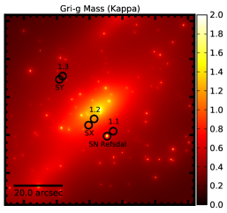
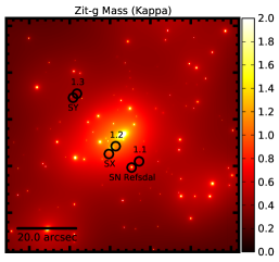
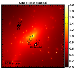
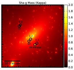
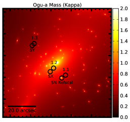
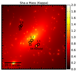
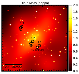
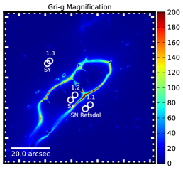
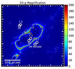
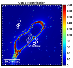

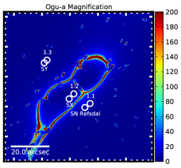
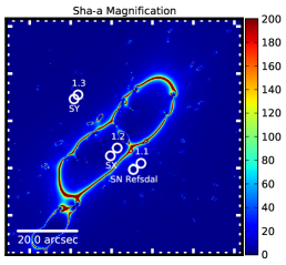
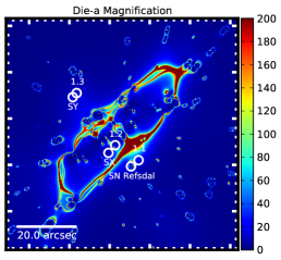
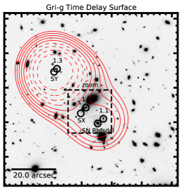
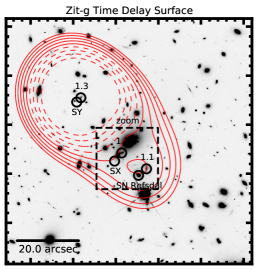

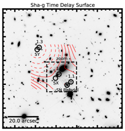
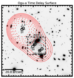
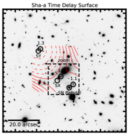
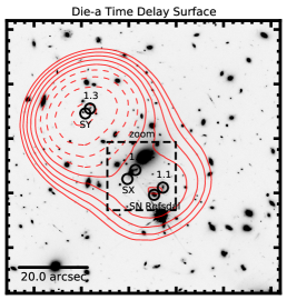
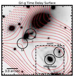
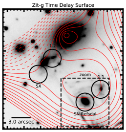
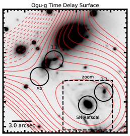
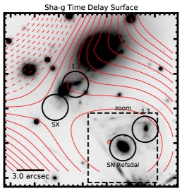


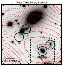
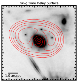
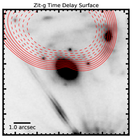
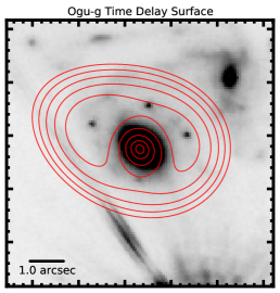
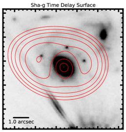
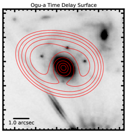
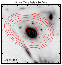
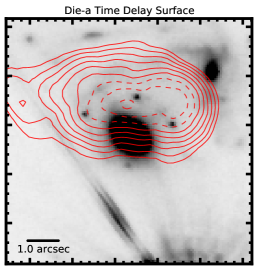
Figure 4 shows the convergence (i.e., surface mass density in units of the lensing critical density) maps. There are striking qualitative differences. The Zit-g map is significantly rounder than the others. The Die-a map has significantly more structure, notably two overdensities near SY/1.3 and at the bottom right of the map. These features were to be expected based on the assumptions used by their methods. The Grillo, Oguri, and Sharon convergence maps are the most qualitatively similar. This is perhaps unsurprising since the three codes are based on fairly similar assumptions.
Magnification maps are shown in Fig. 5. The regions of extreme magnification are qualitatively similar, even though, similarly to the convergence maps, the Zit-g model is overall rounder, while the Die-a model has more structure.
The time-delay surfaces are illustrated at three zoom levels to highlight different features. Fig. 6 shows the global topology of the time-delay surfaces, which is very similar for all models, with minima near 1.1 and SY/1.3 and a saddle point near SX/1.2. As was the case with convergence and magnification, the Zit-g and Die-a time-delay surfaces are rounder and have more structure, respectively, than those produced by the other models.
Zooming in on the region of SX/1.2 and 1.1 in Fig. 7 reveals more differences. The locations of the minimum near SN Refsdal and of the saddle point near 1.2 are significantly different for the Zit-g model, seemingly as a result of the different contribution of the bright galaxy to the NW of 1.2.
A further zoom-in on the region of the known images is shown in Figure 8. The time-delay surface contour levels are shown in step of 10 days to highlight the behavior relevant for the cross configuration. Whereas the “simply-parametrized” models are topologically very similar to each other, the Die-a and Zit-g models are qualitatively different. The time-delay surface is shifted upward, probably as a result of the nearby perturber highlighted in the previous paragraph. We stress that all of the models here are global models, developed to reproduce the cluster potential on larger scales. Hence, local differences should be expected, even though of course they are particularly important in this case.
5.2. Comparing Model Predictions with Measured Time Delays and Magnification Ratios
Before proceeding with a quantitative comparison, we emphasize once again that the uncertainties discussed in this section include only statistical uncertainties. Furthermore, in the comparison we neglect for computational reasons the covariance between the predictions for each of the images, both in time delays and in magnification. Systematic uncertainties will be discussed in Section 6.
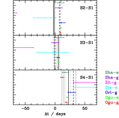
Figure 9 compares the measured time delays with those predicted by the models for the cross configuration. We stress that the measurements were not used in the construction of the models (or known to the modelers), and therefore they can be considered an independent test of the models. The time delay between S2 and S1 (and to some extent that between S3 and S1) is very short, and in fact not all the models agree on the ordering of the two images. The time delay between S4 and S1 is longer and better behaved, with all the models agreeing on the order of the images and with the measured value within the uncertainties. Overall, the models are in reasonable agreement with the measurements, even though formally some of them are in statistical tension. This tension indicates that the uncertainties for some of the parametric models are underestimated.
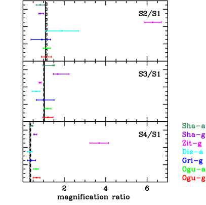
Interestingly, the models appear to predict rather accurately the observed magnification ratios (Fig. 10), even though these quantities should be more sensitive to systematic uncertainties arising from millilensing and microlensing effects than time delays.
Overall, the Zit-g model stands apart from the rest, predicting significantly different time delays and magnification ratios, and larger uncertainties. This qualitative difference is consistent with the different topology of the time-delay surface highlighted in the previous section. Quantitatively, however, the Zit-g model predictions are in broad agreement with the measurements if one considers the 95% credible interval. Collectively, the “simply-parametrized” models seem to predict smaller uncertainties than the others, especially the Ogu-g and Ogu-a ones. This is expected, considering that they have less flexibility than the free-form model. What is surprising, however, is that they also obtain the smaller RMS residual scatter in the predicted vs. observed image positions (Table 4). The Zit-g light-traces-mass model is perhaps the least flexible, in the sense that it cannot account for systematic variations in the projected ratio. This appears to be reflected in its overall largest RMS residual scatter. When comparing the Die-a to the Zit-g model, we note that the former uses significantly more constraints than the latter. This may explain why, even though Die-a is in principle more flexible, it ends up estimating generally smaller uncertainties than Zit-g.
5.3. Forecasts for SN Refsdal: Peak Appearance and Brightness
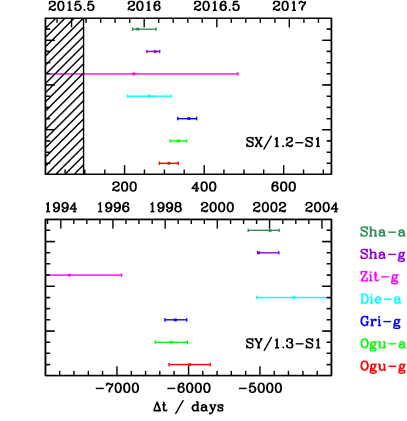
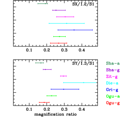
Figure 11 compares the prediction for the next appearance of SN Refsdal, near image 1.2 of the spiral galaxy (hereafter SX/1.2). All the models considered here predict the image to peak between the end of 2015 and the first half of 2016. We note that S1 was first discovered six months before its peak with F160W AB magnitude 25.5 (Kel++15), and it peaked at F160W 24.5 AB (Kelly et al. 2015, in prep.; Rodney et al. 2015, in prep.). Image SX/1.2 is predicted to be approximately 1/3 as bright as image S1 (Figure 12), so it should be 26.7 mag six months before peak and mag at peak. No image is detected in the vicinity of SY/1.3 in data taken with HST up until MACSJ1149.5+2223 became unobservable at the end of July, allowing us to rule out predicted peak times until January 2016.
Remarkably, the models are in excellent mutual agreement regarding the next appearance of SN Refsdal. All of the predictions agree on the first trimester of 2016 as the most likely date of the peak. Sha-a is the only one that predicts a slightly fainter flux with a magnification ratio () as opposed to the 1/3 value predicted by the other models. Interestingly, Zit-g has the largest uncertainty on time delay, but not on magnification ratio. As in the case of the cross configuration, the “simply-parametrized” models yield the smallest uncertainties.
Unfortunately, the model-based estimates of the past appearance of SN Refsdal cannot be tested by observations. The image near 1.3 (hereafter SY/1.3) is estimated to have been significantly fainter than S1, and thus undetectable from the ground, at a time when WFC3-IR was not available. The images of MACSJ1149.5+2223 taken in the optical with ACS in April 2004 (GO-9722, PI Ebeling; 3 limit F814W AB = 27.0 mag) are not sufficiently deep to set any significant constraints, considering the peak brightness of S1 in F814W was 27 mag, and we expect SY/1.3 to be 0.75–2 mag fainter. As a purely theoretical exercise it is interesting to notice that the time delay varies dramatically between models, differing by almost 10 years between the Zit-g and the Sha-a, Sha-g, and Die-a models. Remarkably, and similarly to what was seen for the cross configuration, the magnifications are in significantly better agreement.
6. Discussion
In this section we briefly discuss our results, first by recapitulating the limitations of our analysis (Section 6.1), and then by comparing them with previous work (Section 6.2).
6.1. Limitation of the Blind Test and of the Models
SN Refsdal gives us a unique opportunity to test our models blindly. However, in order to draw the appropriate conclusions from this test, we need to be aware of the limitations of both the test and the models.
The first limitation to keep in mind is that this test is very specific. We are effectively testing point-like predictions of the lensing potential and its derivatives. Similarly to the case of SN “Tomas” (Rod++15), it is very hard to generalize the results of this test even to the strong lensing area shown in our maps. More global metrics should be used to infer a more global assessment of the quality of the models. An example of such a metric is the RMS scatter between the image positions given in Table 4, even though of course even this metric does not capture all of the features of a model. For example, the RMS does not capture how well the model reproduces time delays and magnifications, in addition to positions, and one could imagine trading one for the other.
It is also important to remind ourselves that whereas the magnification and time delays at specific points may vary significantly between models, other quantities that are more relevant for statistical use of clusters as cosmic telescopes, such as the area in the source plane, are much more stable (e.g., Wan+15). And, of course, other quantities such as colors and line ratios are not affected at all by gravitational lensing. It would be interesting to find ways to carry out true observational tests of more global predictions of lens models. One way to achieve this would be to carry out tests similar to those afforded by SN Tomas and SN Refsdal on a large sample of clusters. Another possibility could be to reach sufficiently deep that the statistical properties of the background sources (e.g., the luminosity function) are measured with sufficient precision and small enough cosmic variance to allow for meaningful tests of model uncertainties. Alternatively, tests against simulated data are certainly informative (e.g., Meneghetti et al. 2015, in prep.), although their results should also be interpreted with great care, as they depend crucially on the fidelity of the simulated data and the cross-talk between methods used to simulate the data and those used to carry out the inference.
The second limitation to keep in mind is that the uncertainties listed in this paper are purely statistical in nature. As for the case of image positions — where the RMS scatter is typically larger than the astrometric precision of the image positions themselves (consistent with the fact that there are residual systematics in cluster lens modeling owing to known effects such as substructure, e.g., Bra++09) — we should not expect the time delays and magnifications to be perfectly reproduced by the models either. The spread between the different model predictions gives us an idea of the so-called model uncertainties, even though unfortunately they cannot be considered an exact measurement. The spread could be exaggerated by inappropriate assumptions in some of the models, or underestimated if common assumptions are unjustified.
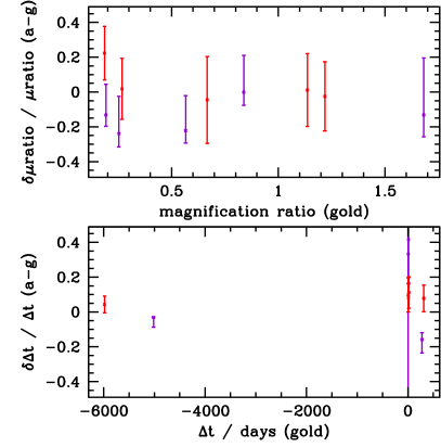
We can use the fact that Oguri et al. and Sharon et al. each submitted two models to estimate the uncertainty relative to the choice of multiple images. By comparing the predictions of the Sha-a and Sha-g and of the Ogu-a and Ogu-g models, we can measure how much the predictions of the models change by adding nonspectroscopically confirmed images to the gold sample, keeping everything else fixed. As shown in Figure 13, the predicted magnification ratios change by less than the statistical uncertainties. The changes in predicted time delays are slightly larger, comparable to the estimated statistical uncertainties, although the relative change in time delays is perhaps not the best metric for the short time delays in the Einstein cross configuration. As can be seen in Figures 9 and 11, the absolute change in predicted time delays is typically within the estimated statistical uncertainties. From this test we conclude that in this case deciding whether to consider a secure but not spectroscopically confirmed set of multiple images introduces an uncertainty that is subdominant with respect to the statistical uncertainties. This is consistent with our expectation that the enlarged set of multiple images does not contain false candidates. In interpreting this result, however, we have to keep in mind the locality of this test and the fact that the nearest images to the observed and predicted images of SN Refsdal are the knots of its host galaxy, all at the same known spectroscopic redshift. Thus, it would have been surprising to find a large difference at these locations.
As already mentioned in the introduction, other potential sources of uncertainty are related to the mass-sheet degeneracy and its generalizations (FGS85; SS13; SS14), the effects of structure along the line of sight (DHB05), and multiplane lensing (S14; Mcc++15). All of the models considered here are single-plane lens models. They break the mass-sheet degeneracy by assuming that the surface mass density profile goes to zero at infinity with a specific radial dependency.
On the scale of the known images of SN Refsdal, the measured time delays and magnification ratios give us a way to estimate these residual uncertainties. The reasonably good agreement between the model prediction and measurements shows that these (systematic) “unknown unknowns” are not dominant with the respect to the (statistical) “known unknowns.” However, since the agreement is not perfect, we conclude that the “unknown unknowns” are not negligible either. We can perhaps use the experience gathered in the study of time delays of lensed quasars to estimate the amplitude of the line-of-sight uncertainties. On scales similar to that of the known images of SN Refsdal, they are believed to be up to % before corrections for galaxies not in clusters (Suy++10; Gre++13; Collett:2013p34320; Suy++14). In numerical simulations, the line-of-sight effects appear to increase with the measured overdensity of galaxies (Gre++13), so it is possible that they are larger for an overdense region like that of MACSJ1149.5+2223.
On galaxy scales, breaking the mass-sheet degeneracy using stellar kinematics and physically motivated galaxy models appears to produce results consistent with residual uncertainties on the order of a few percent (Suy++14). On cluster scales, the degeneracy is partly broken by the use of multiple images at different redshifts (e.g., BLS04). However, in the absence of nonlensing data, we cannot rule out that the residual mass-sheet degeneracy is the dominant source of systematic uncertainty. Assessing the uncertainties related to multiplane effects would require knowledge of the mass distribution in three dimensions and is beyond the scope of the present work. Thus, multiplane lensing cannot be ruled out as a significant source of systematic uncertainty for the prediction of the time delay and magnification ratios of the known images of SN Refsdal. As far as the future image of SN Refsdal is concerned, future observations will tell us how much our uncertainties are underestimated owing to unknown systematics.
Finally, we remind the reader that although for this analysis we kept fixed the cosmological parameters, they are a (subdominant) source of uncertainty. To first order, the time-delay distance is proportional to the Hubble constant, so there is at least a 3% systematic uncertainty (Rie++11; Fre++12) on our predicted time delays (and typically 5–10% when considering all of the other parameters, depending on assumptions and priors; Suy++13; Suy++14).
6.2. Comparison with Previous Models
We can get a quantitative sense of the improvement of the mass models as a result of the new data by comparing how the prediction of the time delay and magnification ratios have changed for the teams who had previously published predictions.
6.2.1 Previous Models by Members of our Team
The Zit-g model updates the models developed by A.Z. for the SN Refsdal discovery paper (Kel++15). The Zit-g model supersedes the estimates of time delays and magnifications given in the original paper by providing predictions as well as quantitative uncertainties.
The update of the Ogu2015 model presented here changes the time delays for S2, S3, S4, SX, SY from 9.2, 5.2, 22.5, 357, days to , , , , days, respectively (for the Ogu-g model, see plot for Ogu-a). Thus, the predicted time delays have changed by less than 1–2, with the inclusion of additional data. The magnification ratios have been similarly stable. The main effect of the additional data has been to reduce the uncertainties.
Die-a & -1719 -4.027 7443 26255 -4521524 1.890.79 0.640.19 0.350.11 0.310.10 0.410.11
Gri-g 10.6 4.8 25.9 361 -6183 0.92 0.99 0.42 0.36 0.30
Ogu-g 8.70.7 5.10.5 18.81.7 31124 -5982287 1.140.24 1.220.24 0.670.17 0.270.05 0.190.03
Ogu-a 9.41.1 5.60.5 20.92.0 33621 -6239224 1.150.17 1.190.17 0.640.11 0.270.03 0.230.03
Sha-g 6 -1 12 277 -5016 0.84 1.68 0.57 0.25 0.19
Sha-a 8 5 17 233 -4860 0.84 1.46 0.44 0.19 0.17
Zit-g -16197 -149113 8251 224262 -7665730 6.270.41 0.830.05 3.690.45 0.310.05 0.300.02