Realization of microwave amplification, attenuation, and frequency conversion using a single three-level superconducting quantum circuit
Abstract
Using different configurations of applied strong driving and weak probe fields, we find that only a single three-level superconducting quantum circuit (SQC) is enough to realize amplification, attenuation and frequency conversion of microwave fields. Such a three-level SQC has to possess -type cyclic transitions. Different from the parametric amplification (attenuation) and frequency conversion in nonlinear optical media, the real energy levels of the three-level SQC are involved in the energy exchange when these processes are completed. We quantitatively discuss the effects of amplification (attenuation) and the frequency conversion for different types of driving fields. The optimal points are obtained for achieving the maximum amplification (attenuation) and conversion efficiency. Our study provides a new method to amplify (attenuate) microwave, realize frequency conversion, and also lay a foundation for generating single or entangled microwave photon states using a single three-level SQC.
pacs:
42.65.Es,42.65.Ky,75.30.CrI Introduction
Three-wave mixing is very fundamental in nonlinear quantum optics NonlinearOptics . It can be used to generate single photon or entangled photon pairs. Three-wave mixing can also be used to convert the frequency of the weak electromagnetic field or amplify the weak electromagnetic signal by virtue of another strong driving field. In atomic systems with inversion symmetry, the three-wave mixing can only occur in a parametric way because of the selection rule in the electric-dipole interaction between the atoms and electric fields. Thus, the nonlinear interaction strength of the three-wave mixing is usually weak in the natural atomic systems. In contrast to the parametric weak nonlinearity realized by the virtual single- or two-photon processes, the nonlinear interaction strength can be increased significantly when the real energy exchange is involved. For example, in molecular systems Three-wave-1977 ; Molecular-book ; Patterson-PRL , the inversion symmetry can be broken, and the transitions between any two energy levels are possible. In such cases, the three-wave mixing processing can be realized using real energy transitions between energy levels. In artificial atoms, e.g., semiconducting quantum dots or superconducting quantum circuits (SQCs), the inversion symmetry of their potential energy can be artificially controlled by externally applied field, that is, the selection rule of the artificial atoms can be engineered. Thus, they provide us a new platform to manipulate and engineer linear and nonlinear quantum processes. For example,the single photon strong coupling can be achieved between microwave and mechanical modes using a superconducting flux qubit ZYXue-APL . It is also possible to realize three-wave mixing using real energy transitions between energy levels of a single SQC liuyx .
The SQCs RMP ; wendin ; clarke ; xiang ; you-today ; you-nature ; Girvin-review are extensively explored for the realization of qubits which are basic building blocks of quantum information processing. These superconducting artificial atoms can also be used not only to demonstrate phenomena occurred in atomic physics and quantum optics, but also to show some novel results, which cannot be found in natural atomic systems. For example, the dressed states liu2006 ; Cohen-Tannoudjibook have been experimentally demonstrated using superconducting charge qubit circuits delsing2007 ; delsing2010 . The Autler-Townes splitting atsET ; atsEP ; atsEP1 ; atsEF ; Bsanders ; atsET-2 ; atsET-3 and coherent population trapping CPT have also been observed in three-level SQCs. Experimentalists are trying to find a way to realize the electromagnetically induced transparency in varieties of three-level superconducting quantum devices CPYang ; murali ; dutton ; HouIan ; huichen Sun . Moreover, the coexistence of single- and two-photon processes liuprl in three-level superconducting flux qubit circuits liuprl ; orlando has been experimentally demonstrated naturephysics2008 by designed circuit QED systems. However, such phenomenon cannot be demonstrated using three-level natural atoms because of the electric-dipole transition rule.
The microwave amplification has been experimentally demonstrated by a single three-level artificial atom in open one-dimensional space Olig , a dressed Ilichev or a doubly-dressed superconducting flux Ilichev1 qubit circuit. The coherent frequency conversion has be demonstrated using two internal degrees of freedom of a single dc-SQUID phase qubit circuit Bussion . The parametric down conversion and squeezing of two-mode quantized microwave fields using circuit QED are theoretically studied KMoon . Moreover, the parametric three-wave mixing devices have also been experimentally demonstrated devoret1 ; devoret2 . It was shown that the amplifiers with single artificial atoms Olig are different from the Josephson junction based parametric three-wave mixing devices devoret1 ; devoret2 or amplifiers A1 ; A2 ; A3 ; A4 . A main difference is that the real energy exchange between discrete energy levels is involved when the single artificial atom amplifiers are implemented. We recently showed that a three-level flux qubit circuits liuyx with -type cyclic transitions can be used to generate three-wave mixing.
Motivated by the work Olig ; liuyx , we now give a detailed study on the microwave amplification and frequency conversion by a single three-level SQC with -type transitions, which can be realized by superconducting flux orlando ; liuprl , phase Martinis ; Hakonen1 ; Hakonen2 , fluxoniumfluxonium1 ; fluxonium2 or Xmon qubit circuits Xmon . For concreteness, we here focus on flux qubit circuits. In our study, we mainly study the conversion efficiency and the amplification and attenuation of the weak signal field. Our paper is organized as follows. In Sec. II, we give an overview of the theoretical model. In Sec. III, we study the microwave attenuation and frequency conversion for driving type (1). In Sec. IV, we study the same contents for driving type (2). In Sec. V, we study microwave amplification, attenuation, and frequency conversion for driving type (3). Finally, we summarize our results and discuss both measurements and experimental feasibilities.
II Theoretical model overview
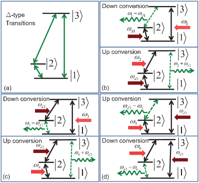
We study microwave amplifications, attenuation and frequency conversions in a three-level superconducting artificial atom with -type transitions liuprl , as schematically shown in Fig. 1(a). The three energy levels are denoted by , , and . Here, we specify our study to superconducting flux qubit circuits, typically consisting of three Josephson junctions orlando ; liuprl . We assume that the bias magnetic flux is not at the optimal point so that the three energy levels chosen from such circuit can possess -type transition when the external fields are applied. We also assume that the three-level system is placed inside an open one-dimensional transmission line resonator as in Ref. Olig . Hereafter, for simplicity, we use three-level systems to denote such three-level superconducting flux qubit circuits.
To realize the microwave amplification, attenuation, or frequency conversion, a strong driving field has to be applied to the three-level system with -type transitions, as shown in Figs. 1(b), (c) and (d), the strong driving field can be applied to couple: (1) the energy levels and ; or (2) the energy levels and ; or (3) the energy levels and . Corresponding to each configuration of the driving field, the signal field can be applied in two ways. For example, as shown in two panels of Fig. 1(b), the signal field can be applied to either the energy levels and (shown in up panel of Fig. 1(b)), or the energy levels and (shown in down panel of Fig. 1(b)) when the driving field is applied to the energy levels and .
In strong driving types (1) and (2) as shown in Figs. 1(b) and (c), the frequency down or up conversion can be realized by properly applying the signal field. But in the driving type (3) as shown in Fig. 1(d), the up and down conversions are a little bit different from the types (1) and (2). In the types (1) and (2), the down (up) frequency conversion is the difference between (sum of) frequencies of the signal and driving fields. However, in the type (3), both the down and up frequency conversions are the difference between the frequencies of signal and driving fields, when the frequency difference is larger than the signal frequency, we call this process as the up conversion, otherwise the down conversion.
In all three driving ways with applied signal fields, the total Hamiltonian can be generally given by
| (1) |
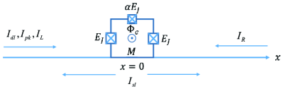
from Ref. liuyx when one of the weak fields is replaced by a strong field. We note that we sometimes also call signal fields as probing fields. Hereafter, with , or . The superscript , or is used to represent different driving types. The Hamiltonian can be exemplified by the circuit schematic in Fig. 2 where the signals applied through the transmission line will be scattered by the flux qubit as in Ref. nec2010science . In the type of the th driving, the symbol (or ) denotes the interaction Hamiltonian between the strong driving field (or the weak signal field) and the three-level system. The Hamiltonian
| (2) |
describes the interaction between the three-level system and environment in open one-dimensional transmission line. In Eq. (2), we have used the two following symbols
| (3) | ||||
| (4) |
with for the noise currents coming from the left and right. The parameter represents the characteristic impedence of the transmission line. The commutation relations of are for or . Without the driving fields, the relaxation rates of the three-level system are proportional to the parameters
| (5) |
All the types of interaction Hamiltonians and have been summarized in Table 1.
Our research is based on the following hypotheses. (1) The intrinsic loss of the three-level system is negligible. Hence, the 1D open space determines the total decay rates. (2) The frequency shifts induced by the driving field are much larger than the decay rates but still negligibly small compared to the original eigen frequencies of the three-level system. (3) The interaction Hamiltonian between the flux qubit circuit and the probe field is a small quantity compared with that between the flux qubit circuit and the driving field . Thus, the response to the probe signal can be solved using linear response theory NonlinearOptics . (4) The environment temperature is too enough to induce effective dephasing or thermal excitation.
Below we will first use driving type (1) as an example to show detailed derivations. The treatments in driving type (2) and (3) are similar to that in driving type (1).
| Driving type | Interaction Hamiltonian with the driving field | Interaction Hamiltonian with the probe field |
|---|---|---|
| Type (1) | ||
| Type (2) | ||
| Type (3) |
III Microwave attenuation and frequency conversions for driving type (1)
III.1 Hamiltonian reduction
In the driving type (1), the Hamiltonian can be given as
| (6) |
with Here is the mutual inductance, and is the matrix element of the loop current of the three-level superconducting flux qubit circuit. The incident driving current is assumed as with phase velocity . We assume that the three-level system is placed at the position of and also is a real number without loss of generality.
Corresponding to the Hamiltonian in Eq. (6), the Hamiltonian with or 2 are respectively
| (7) | ||||
| (8) |
without the rotating wave approximation (RWA). The Hamiltonian in Eq. (1) with in Eq. (6) and in Eq. (7) describes the frequency down conversion as shown in the up panel of Fig. 1(b). However, the Hamiltonian can be written as for that the signal field is applied to the energy levels and . That is, the Hamiltonian in Eq. (1) with in Eq. (6) and in Eq. (8) describes the frequency up conversion as shown in the down panel of Fig. 1(b). The incident signal currents are assumed as with or .
To remove the time dependence of , we now use a unitary transformation . Then at a frame rotating, we get an effective Hamiltonian
| (9) | ||||
with driving detuning and the transformed loop current . Since we have assumed a strong driving strength , it is reasonable to work in the eigen basis of the first three terms of Eq. (9). For this consideration, we apply to a unitary transformation with , yielding
| (10) |
The symbols , , respectively take the following forms, i.e.,
| (11) | ||||
| (12) | ||||
| (13) |
Note that is another transformed loop current. Its matrix elements have been listed in Appendix. A. The Hamiltonian is defined as the system Hamiltonian originating from the first three terms of in Eq. (9). In Eq. (11), the eigen frequencies of the system Hamiltonian are respectively represented as
| (14) | ||||
| (15) | ||||
| (16) |
The Hamiltonian is a small quantity compared to and hence will be treated as a perturbation in the following discussions. And represents the interaction between the system and 1D open space. With fast oscillating terms neglected, can be further reduced to
| (17) | ||||
| (18) |
Here, is the produced sum frequency, and
| (19) | ||||
| (20) | ||||
| (21) | ||||
| (22) |
are the coupling energy parameters.
III.2 Dynamics of the system and its solutions
Using the detailed parameters of in Appendix. A, we can derive that the reduced density matrix of the system is governed by the following master equation QN3
| (23) |
We must mention we work in the picture defined by unitary transformations and . The dissipation of the system is described via the Lindblad term
| (24) |
Here, are matrix elements of the reduced density operator . The relaxation and dephasing rates can be calculated as and from hypotheses (1), (2), and (4) in Sec. II. The explicit expressions of and are given in Appendix A.
It is not easy to obtain the exact solutions of the nonlinear equations in Eq. (23) because the steady state response contains infinite components of different frequencies in nonlinear systems. Thus, as extensively used method in nonlinear optics NonlinearOptics , we now seek the solutions of Eq. (23) in the form of a power series expansion in the magnitude of , that is, a solution of the form
| (25) |
for the reduced density matrix of the three-level system. Here, is the steady state solution when no signal field is applied to the system. However the th-order reduced density matrix is proportional to th order of .
In the first order approximation, we have
| (26) | ||||
| (27) |
The solutions of Eq. (26) is
| (28) | ||||
| (29) |
with . And the other terms of are all zeros. Having obtained , we can further solve Eq. (27). When takes , we have the nonzero matrix elements of as follows,
| (30) | ||||
| (31) |
When takes , we have the nonzero matrix elements of as follows,
| (32) | ||||
| (33) |
III.3 Scattered current
The noise current ( and ) will induce the scattered current of the classical fields through interaction with the three-level system. Using the input-output theory extensively discussed in Refs. QN1 ; QN2 ; QN3 ; QN4 ; QN5 , the scattered current at can be represented by
| (34) |
with , and . Here, we have assumed that the matrix element of is of the form . The scattered current can also be expanded in the order of , i.e., . Here, we only care about the linear response in the expansion of , that is,
| (35) |
III.4 Probe type (1)
When takes using Eqs. (30)-(31), we have the linear response as
| (36) |
where is the produced difference frequency. The amplitudes of both frequency components are respectively denoted as and . The gain of the incident current is defined as , and the explicit expression is
| (37) |
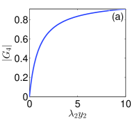
Meanwhile, the corresponding efficiency of frequency down conversion is defined as since represents the photon number of frequency produced by each photon of frequency per unit time. Then, the explicit expression of can be reduced to
| (38) |
The two resonant points of and are respectively at and . As is assumed larger than the decay rates, the two resonant points must be well separated. Therefore, we can determine from Eq. (37) that the transmitted signal with frequency can only be attenuated. At both points, ( reaches their minimum (maximum) values respectively. To obtain the optimal attenuation or conversion efficiency, we can first minimize and where
| (39) | ||||
| (40) |
The dephasing rates and can be further reduced to
| (41) | ||||
| (42) |
in the limit that and . We thus assume and in the following discussions of and .
We now further seek the limitation value of when . In this case, is reduced to
| (43) |
where . Apparently, when and , the optimal gain for attenuation can reach
| (44) |
In the resonant driving case, , and the best gain for attenuation can reach
| (45) |
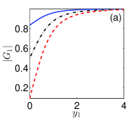
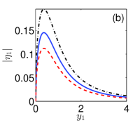
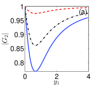
under the condition In Fig. 3(a), takes Eq. (43). We have plotted as functions of when takes 0.2, 1, and 10, respectively. It can be easily seen that will decrease as increases or decreases. It is a similar case when , where the gain becomes
| (46) |
The similarity can be easily found between Eqs. (43) and (46). Thus, we directly have the optimal gain for attenuation
| (47) |
when and . In the resonant driving case, , and the optimal gain for attenuation can reach
| (48) |
with the condition . The properties of when takes (46) can also be investigated through Fig. 3(a).
We now seek the limitation of when . In this case, is reduced to
| (49) |
It can be proved that when and , the optimal conversion efficiency reads
| (50) |
In the resonant driving case, , and we have the optimal conversion efficiency
| (51) |
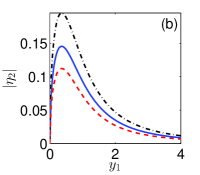
under the condition . In Fig. 3(b), takes Eq. (49)̇. We have plotted as functions of when takes 0.2, 1, and 10, respectively. As is given and increases, first increases to the maximum point and then fall towards zero. Given , the maximum emerges at . It is a similar case when , where the conversion efficiency becomes
| (52) |
The similarity can be easily found between Eqs. (49) and (52). Thus, the optimal conversion efficiency reads
| (53) |
when and . In the resonant driving case, i.e., , we have the optimal conversion efficiency
| (54) |
also under the condition . The properties of when takes (52) can also be investigated through Fig. 3(b).
III.5 Probe type (2)
When takes using Eqs. (32)-(33), we have the linear response as
| (55) |
The amplitudes of both frequency components are respectively and . The gain of the incident current is defined as , and the explicit expression is
| (56) |
Meanwhile, the corresponding efficiency of frequency down conversion is defined as since represents the photon number of frequency produced by each photon of frequency per unit time. The explicit expression of is hence
| (57) |
The two resonant points of and are respectively at and . As we have assumed a sufficiently large , the two resonant points must be well separated. Therefore, we can know from Eq. (56) that the transmitted signal with frequency can only be attenuated. At both points, ( reaches their minimum (maximum) values respectively. As in probe type (1), we should also assume and in the following discussions for achieving optimal and .
We now further seek the limitation value of when . In this case, is reduced to
| (58) |
It can be proved that when , and , we can achieve the optimal gain for attenuation, that is,
| (59) |
In the resonant driving case, i.e., , the optimal gain for attenuation can reach
| (60) |
under the condition . In Fig 4(a), takes Eq. (58). We have plotted as functions of when takes 0.2, 1, and 10, respectively. When increases, will first decrease until meeting the minimum point and then switch to increase. As increases, will also increase. It is a similar case when , where the gain becomes
| (61) |
The similarity can be easily found between Eqs. (58) and (61). Thus we can obtain that when and , the optimal gain for attenuation reads
| (62) |
In the resonant driving case, i.e., , we have the optimal gain for attenuation
| (63) |
under the condition . When takes Eq. (61), can also be investigated through Fig 4(a).
We now seek the limitation of when . In this case, is reduced to
| (64) |
We find that Eqs. (64) and (49) are exactly of the same form. We thus directly give that when and , the optimal conversion efficiency reads
| (65) |
In the resonant driving case, , and the optimal conversion efficiency reads
| (66) |
when . It is a similar case when , where the conversion efficiency becomes
| (67) |
The similarity can be easily found between Eqs. (64) and (67). We hence obtain that when and , the optimal conversion efficiency reads
| (68) |
In the resonant driving case, , and the optimal conversion efficiency reads
| (69) |
when . For completeness, we also plot Fig. 4(b) for . Whether takes Eq. (64) or (67), the behaviours of can be investigated through Fig. 4(b).
IV Microwave attenuation and frequency conversions for driving type (2)
IV.1 Hamiltonian reduction
In the driving type (2), the Hamiltonian can be given as
| (70) |
with The incident driving current is assumed as with the phase velocity . We assume that is a real number without loss of generality.
Corresponding to the Hamiltonian in Eq. (70), the Hamiltonian with or 4 are respectively
| (71) | ||||
| (72) |
without RWA. The Hamiltonian in Eq. (1) with in Eq. (70) and in Eq. (71) describes the frequency down conversion as shown in the up panel of Fig. 1(c). However, the Hamiltonian can be written as for that the signal field is applied to the energy levels and . That is, the Hamiltonian in Eq. (1) with in Eq. (70) and in Eq. (72) describes the frequency up conversion as shown in the down panel of Fig. 1(c). The incident signal currents are assumed as with or .
To remove the time dependence of , we now use a unitary transformation . Then at a frame rotating, we get an effective Hamiltonian
| (73) |
with driving detuning and the transformed loop current . Furthermore, we think driving strengths are strong enough compared to the decay rates of the flux qubit circuit. Then, we should work in the eigen basis of the first three terms of Eq. (73). Thus, we apply to a unitary transformation with , yielding
| (74) |
where
| (75) | ||||
| (76) | ||||
| (77) |
Note that is another transformed loop current and its matrix elements have been listed in Appendix. B. Here, is treated as the system Hamiltonian originating from the first three terms in Eq. (73). In Eq. (75), the eigen frequencies are respectively
| (78) | ||||
| (79) |
The Hamiltonian is a small quantity compared to and hence will be treated as the perturbation to the system Hamiltonian. Besides, determines the dissipation of the system into the 1D open space. Without fast oscillating terms neglected, can be further reduced to
| (80) | ||||
| (81) |
where is the produced difference frequency, and the coupling energy parameters are
| (82) | ||||
| (83) | ||||
| (84) | ||||
| (85) |
IV.2 Dynamics of the system and its solutions
Using the detailed parameters of in Appendix. B, we can derive that the reduced density matrix of the system is governed by the following master equation QN3
| (86) |
We must mention we work in the picture defined by unitary transformations and . The dissipation of the system is described via the Lindblad term
| (87) |
Here, are matrix elements of the reduced density operator . The relaxation and dephasing rates can be calculated as and from hypotheses (1), (2), and (4) in Sec. II. The explicit expressions of and are given in Appendix. B.
Then we seek the solutions of Eq. (86) in the form of a power series expansion in the magnitude of , that is, a solution of the form
| (88) |
for the reduced density matrix of the three-level system. Here, is the steady state solution when no signal field is applied to the system. However the th-order reduced density matrix is proportional to th order of .
In the first order approximation, we have
| (89) | ||||
| (90) |
The solutions of Eq. (89) is
| (91) |
And the other terms of are all zeros. Having obtained , we can future solve Eq. (90). When takes , we have the nonzero matrix elements of as follows,
| (92) | ||||
| (93) |
When takes , we have the nonzero matrix elements of as follows,
| (94) | ||||
| (95) |
IV.3 Scattered current
The scattered current at , similarly to driving type (1), can be represented by
| (96) |
with . Here, we have assumed that the matrix element of is of the form . We hereby also expand the scattered current as , where is in the th order of . In this paper, we only care about the linear response of , that is,
| (97) |
IV.4 Probe type (3)
When takes using Eqs. (94)-(95), we have the linear response as
| (98) |
where is the produced difference frequency. The amplitudes of both frequency components are respectively and . The gain of the incident current is defined as , and the explicit expression is
| (99) |
Meanwhile, the corresponding efficiency of frequency down conversion is defined as since represents the photon number of frequency produced by each photon of frequency per unit time. The explicit expression of is hence
| (100) |
The two resonant points of and are respectively at and . As we have assumed a sufficiently large , the two resonant points must be well separated. Therefore, we can determine from Eq. (99) that the transmitted signal with frequency can only be attenuated. At both points, ( reaches their minimum (maximum) values respectively. To obtain the optimal attenuation or conversion efficiency, we can first minimize and where
| (101) | ||||
| (102) |
The dephasing rates and can be further reduced to
| (103) | ||||
| (104) |
in the limit that and . We thus assume and in the following discussions of and .
We now further seek the limitation value of when . In this case, is reduced to
| (105) |
with . Apparently, when , the optimal gain for attenuation reads
| (106) |
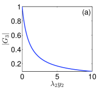
In the resonant driving case, , and the optimal attenuation is also achievable with . In Fig. 5(a), takes Eq. (105). We have plotted as a function of . When increases, also shows decrease towards zero. It is a similar case when , where the gain becomes
| (107) |
The similarity can be easily found between Eqs. (105) and (107). Thus, the optimal gain for attenuation reads
| (108) |
when the condition is satisfied. In the resonant driving case, , and the optimal gain for attenuation is also achieved with . When takes Eq. (107), the properties of can also be investigated through Fig. 5(a).
We now seek the limitation of when . In this case, is reduced to
| (109) |
When , the optimal conversion efficiency reads
| (110) |
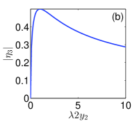
In the resonant driving case, , and the optimal conversion efficiency is also achievable when . In Fig. 5(b), takes Eq. (109). We have plotted as a function of . When increases, we find that first increases to the optimal point and then falls towards zero. It is a similar case when , where the conversion efficiency reads
| (111) |
The similarity can be easily found between Eqs. (111) and (109). When , we have the optimal conversion efficiency
| (112) |
In the resonant driving case, , and the optimal conversion efficiency is also accessible with . When takes Eq. (111), the property of can be similarly investigated through Fig. 5(b).
IV.5 Probe type (4)
When takes using Eqs. (94)-(95), we have the linear response as
| (113) |
The amplitudes of both frequency components are respectively and . The gain of the incident current is defined as , and the explicit expression is
| (114) |
Meanwhile, the corresponding efficiency of frequency down conversion is defined as since represents the photon number of frequency produced by each photon of frequency per unit time. The explicit expression of is hence
| (115) |
The two resonant points of and are respectively at and . As we have assumed a sufficiently large , the two points must be well separated. Therefore, we can determine from Eq. (114) that the transmitted signal with frequency can only be attenuated. At both points, () reaches their minimum (maximum) values respectively. In the following discussions, we will similarly assume and just as in probe type (3).
We now further seek the limitation value of when . In this case, is hence reduced to
| (116) |
When , we have the optimal gain for attenuation reading
| (117) |
In the resonant driving case, , and the optimal gain for attenuation is also achievable when . In Fig. 6(a), takes 114. We have plotted as the function of . When increase, exhibits increase towards one. It is a similar case when , where the gain becomes
| (118) |
The similarity can be easily seen between Eqs. (118) and (116). Thus when , the optimal gain attenuation reads
| (119) |
In the resonant driving case, , and the optimal attenuation is also with . When takes Eq. (118), the behaviours of can be similarly explained through Fig. 6(a).
We now seek the limitation of when . In this case, the conversion efficiency is reduced to
| (120) |
Apparently, Eqs. (120) and (109) are of the same form. We hence directly have that when the optimal conversion efficiency reads
| (121) |
In the resonant driving case, , and the optimal conversion efficiency is also with . It is a similar case when , where
| (122) |
When , the optimal conversion efficiency reads
| (123) |
In the resonant driving case, , and the optimal conversion efficiency is also with . For completeness, we also plot Fig. 6(b) for . Whether takes Eq. (120) or (122), the behaviours of can be investigated through Fig. 6(b).

V Microwave amplification, attenuation, and frequency conversions in the driving type (3)
According to the analysis on the frequency conversion and the properties of the output signal field in both driving types (1) and (2). We find that the signal fields can only be attenuated and not be amplified in both cases. However the frequency conversion can be realized. We now study the frequency conversion and the amplification (or attenuation) of incident signal field for the driving type (3), in which the energy levels and are driven by the strong pump field, and the signal field is used to couple either the energy levels and or the energy levels and . In this driving case, we find that the incident signal field can be amplified. The detailed analysis is given below.
V.1 Hamiltonian reduction
In the driving type (3), the Hamiltonian can be given as
| (124) |
with The incident driving current is assumed as with the phase velocity . The strength is assumed as a real number without loss of generality.
Corresponding to the Hamiltonian in Eq. (124), the Hamiltonian with or 6 are respectively
| (125) | ||||
| (126) |
without RWA. The Hamiltonian in Eq. (1) with in Eq. (124) and in Eq. (125) describes the frequency up conversion as shown in the up panel of Fig. 1(d). However, the Hamiltonian can be written as for that the signal field is applied to the energy levels and . That is, the Hamiltonian in Eq. (1) with in Eq. (70) and in Eq. (126) describes the frequency down conversion as shown in the down panel of Fig. 1(c). The incident signal currents are assumed as with or .
To remove the time dependence of , we now use a unitary transformation . Then at a frame rotating, we get an effective Hamiltonian
| (127) |
with driving detuning and loop current . Furthermore, we think driving strengths are strong enough compared to the decay rates of the flux qubit circuit. Then, we should work in the eigen basis of the first three terms of Eq. (127). Thus, we apply to a unitary transformation with yielding
| (128) |
where
| (129) | ||||
| (130) | ||||
| (131) |
Here, the loop current and its matrix elements have been listed in Appendix. C. Here, is treated as the system Hamiltonian originating from the first three terms in Eq. (73). In Eq. (75), the eigen frequencies are respectively
| (132) | ||||
| (133) | ||||
| (134) |
The Hamiltonian is a small quantity compared to and hence will be treated as the perturbation to the system Hamiltonian. Besides, determines the dissipation of the system into the 1D open space. With fast oscillating terms neglected, can be further reduced to
| (135) | ||||
| (136) |
where is the produced difference frequency, and the coupling energy parameters are
| (137) | ||||
| (138) | ||||
| (139) | ||||
| (140) |
V.2 Dynamics of the system and its solutions
Using the detailed parameters of in Appendix. C, we can derive that the reduced density matrix of the system is governed by the following master equation QN3
| (141) |
We must mention we work in the picture defined by unitary transformations and . The dissipation of the system is described via the Lindblad term
| (142) |
Here, are matrix elements of the reduced density operator . The relaxation and dephasing rates can be calculated as and from hypotheses (1), (2), and (4) in Sec. II. The explicit expressions of and given in Appendix. C.
Then we seek the solutions of Eq. (86) in the form of a power series expansion in the magnitude of , that is, a solution of the form
| (143) |
for the reduced density matrix of the three-level system. Here, is the steady state solution when no signal field is applied to the system. However, the th-order reduced density matrix is proportional to th order of .
In the first order approximation, we have
| (144) | ||||
| (145) |
The solutions of Eq. (144) are
| (146) | ||||
| (147) | ||||
| (148) |
all of which are independent. And the other terms of are all zeros. Having obtained , we can future solve Eq. (145). When takes , we have the nonzero matrix elements of as follows,
| (149) | ||||
| (150) |
when takes , we have the nonzero matrix elements of as follows,
| (151) | ||||
| (152) |
V.3 Scattered current
The scattered current at , similarly to driving type (1), can be represented by
| (153) |
with . Here, we have assumed that the matrix element of is of the form . We hereby also expand the scattered current as , where is in the th order of . In this present paper, we are only interested in the linear response of , that is,
| (154) |
V.4 Probe type (5)
When takes using Eqs. (149)-(150), we have the linear response as
| (155) |
where is the produced difference frequency. The amplitudes of both frequency components are respectively and . The gain of the incident current is defined as , and the explicit expression is
| (156) |
Meanwhile, the corresponding efficiency of frequency down conversion is defined as since represents the photon number of frequency produced by each photon of frequency per unit time. The explicit expression of is hence
| (157) |
The two resonant points of and are respectively at and . As we have assumed a sufficiently large , the two points must be well separated. Therefore, we can determine from Eq. (156) that the transmitted signal with frequency can be both attenuated and amplified depending on the sign of or . At both points, reaches the maximum or minimum gain, while reaches the maximum conversion efficiency. To obtain the optimal attenuation, amplification, or conversion efficiency, we can first minimize and whose expressions are respectively
| (158) | ||||
| (159) |
Here, . The dephasing rates and can be further reduced to
| (160) | ||||
| (161) |
in the limit that and . We thus assume and in the following discussions of and .
When is near , the amplification condition (i.e., is
| (162) |
and the attenuation condition (i.e., is
| (163) |
We now further seek the limitation value of when . In this case, is reduced to
| (164) |
with . In Eq. (164), and will be regarded as independent parameters. In the amplification case, can be maximized, yielding
| (165) |
when the condition holds. Here, parameters and respectively take and . Furthermore, the condition yields the optimal amplification, yielding
| (166) |
where the condition for becomes . In the resonant driving case, using Eq. (165), the optimal for amplification can be reduced to
| (167) |
where the conditions become and . In the attenuation case, can be minimized, yielding
| (168) |
when . Furthermore, the condition yields the optimal gain for attenuation, that is,
| (169) |
In the resonant driving case, from Eq. (168), the optimal for attenuation can be reduced to
| (170) |
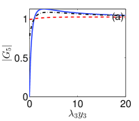
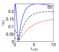
where the conditions are and . In Fig. 7(a), takes Eq. (164). We have plotted as the function of when takes 0, 1, and 4, respectively. When increases from , to , and then to , sequentially exhibits attenuation (), transparency (), and amplification (). Despite the regime of , the increase of will always weaken the attenuation or amplification of the probe signal.
When is near , The amplification condition (i.e., ) is
| (171) |
and the attenuation condition (i.e., is
| (172) |
We now further seek the limitation value of when . In this case, is reduced to
| (173) |
The similarity can be easily seen between Eqs. (173) and (164). We thus directly have that in the amplification case, the gain for amplification can be maximized as
| (174) |
when with , . Furthermore, optimal gain for amplification can be achieved as
| (175) |
when and . From Eq. (174), the optimal gain for amplification can be reduced to
| (176) |
in the resonant driving case where the conditions are , and . In the attenuation case, the gain for attenuation can be minimized as
| (177) |
when . Furthermore, the condition yields the optimal gain for attenuation, that is,
| (178) |
From Eq. (177), the optimal for attenuation can be reduced to
| (179) |
in the resonant driving case where the condition are and . The behaviours of can be similarly explained through Fig. 7(a) when takes Eq. (173).
We now seek the limitation of when . In this case, the conversion efficiency is reduced to
| (180) |
Here, and will be continuously treated as independent. When , the conversion efficiency can be maximized as
| (181) |
Furthermore, the condition yields the optimal conversion efficiency as
| (182) |
In the resonant driving case, , and the optimal conversion efficiency reads
| (183) |
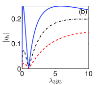
under the condition . In Fig. 7(b), takes Eq. (180). We have plotted as the functions of when takes 0, 1, and 2, respectively. When , we can see , indicating the switch off of conversion process. Besides this point, there are two peaks. When , the two peaks are of the same value. When takes 1 and 2, the peak at the right takes the largest value. Besides, the larger value takes, the smaller becomes. It is a similar case when , where the conversion efficiency becomes
| (184) |
The similarity can be easily found between Eqs. (184) and (180). Thus, it can be directly given that at and , the optimal conversion efficiency reads
| (185) |
In the resonant driving case, , and the optimal conversion efficiency reads
| (186) |
when . When takes Eq. (184), the behavious of can also be explained though Fig. 7(b).
V.5 Probe type (6)
When takes using Eqs. (151)-(152), we have the linear response as
| (187) |
The amplitudes of both frequency components are respectively and . The gain of the incident current is defined as , and the explicit expression is
| (188) |
Meanwhile, the corresponding efficiency of frequency down conversion is defined as since represents the photon number of frequency produced by each photon of frequency per unit time. The explicit expression of is hence
| (189) |
The two resonant points of and are respectively at and . As we have assumed a sufficiently large , the two points must be well separated. Therefore, we can determine from Eq. (56) that the transmitted signal with frequency can be both attenuated or amplified. At both points, reaches the maximum gain and maximum conversion efficiency, while reaches the maximum conversion efficiency. We will similarly assume and as in probe type (5) in the following discussions of and .
We now further seek the limitation value of when . In this case, is reduced to
| (190) |
In the amplification case, the gain can be maximized as
| (191) |
when with , and . Furthermore, the condition yields the optimal gain for amplification, i.e.,
| (192) |
where the condition for becomes . From Eq. (191), the optimal gain for amplification can be reduced to
| (193) |
in the resonant case, where the conditions are and . In the attenuation case, the condition yields the optimal gain for attenuation
| (194) |
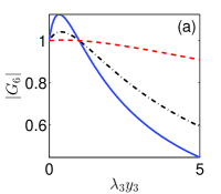
In the resonant driving case, the conditions become and where the optimal gain for attenuation is still . In Fig. 8, takes Eq. (190). We have plotted as the function of when takes 0, 1, and 4, respectively. When changes from , to , and then to , sequentially exhibits amplification (), transparency (), and attenuation (). Despite the regime of , the increase of will always weaken the attenuation or amplification of the probe signal. It is a similar case when , where the gain becomes
| (195) |
The similarity can be easily found between Eqs. .(195) and (190). Thus, we directly have that the gain for amplification can be optimized as
| (196) |
when with , , , and . Furthermore, the condition yields the optimal gain for amplification
| (197) |
where From Eq. (196), the gain for amplification can be reduced to
| (198) |
with the condition and . In the attenuation case, the condition yields the optimal gain as
| (199) |
In the resonant case, the conditions become and where the optimal gain for attenuation is still . When takes Eq. (195), the behaviour of can also be investigated through Fig. 195(a).
We now seek the limitation of when . In this case, is reduced to
| (200) |
We find Eqs. (200) and (180) are equivalent except for a global constant. We thus directly have the optimal conversion efficiency
| (201) |
when and . In the resonant driving case, , and the optimal conversion efficiency becomes
| (202) |
in the condition that . It is a similar case when , where the conversion efficiency becomes
| (203) |
With the condition and , the optimal conversion efficiency reaches
| (204) |
In the resonant driving case, , and we can achieve the optimal conversion efficiency as
| (205) |
when . For completeness, we also plot Fig. 8(b). Both Eqs. (200) and (203) can be described by Fig. 8(b).
VI Conclusions and Discussions
In summary, using a three-level three-junction flux qubit circuit as an example, we study how the frequency conversion and signal amplification (or attenuation) can be realized when the inversion symmetry of the potential energy is broken. We mention that the microwave amplification has recently been experimentally realized Olig ; nec2010science in a three-level system constructed by four-junction flux qubit circuits. However, our study provides a full picture for understanding the microwave frequency conversion and amplification (or attenuation) in the case of all possible driving and probing. As a summary, we list in Table. 2 the maximum (or minimum) gains and maximum conversion efficiencies at different driving and probe types. The conditions for achieving these values are also appended in this table.
Based on different configurations of the applied driving and probing fields, we classify our study into three types. We find that a single three-level superconducting flux qubit circuit is enough to complete the microwave frequency conversion, amplification (or attenuation) of weak signal fields. In particular, we find, (i) in the driving types (1) and (2), the three-level system can convert the driving and signal fields into the ones with new frequencies, which we call down conversion or up conversion, respectively. Due to the energy loss in the reflection and conversion, the incident signal field suffers the attenuation after transmitted in these two driving types; (ii) however, both amplification and attenuation can occur in the driving type (3), whether the amplification or the attenuation depends on the parameter condition; (iii) given a definite flux bias, when the driving and signal detunings are adjusted properly, the maximum conversion efficiencies and gains nearly do not depend on the driving strength.
| Detuned driving | Resonant driving | Detuned driving | Resonant driving | ||||||||
| 1 | 1 | 0 | |||||||||
| 1 | 1 | 0 | |||||||||
| 1 | 2 | ||||||||||
| 1 | 2 | ||||||||||
| 2 | 3 | 0 | 0 | ||||||||
| 2 | 3 | 0 | 0 | ||||||||
| 2 | 4 | 0 | 0 | ||||||||
| 2 | 4 | 0 | 0 | ||||||||
| 3 | 5 | ||||||||||
| 3 | 5 | 0 | - | - | - | - | |||||
| 3 | 5 | ||||||||||
| 3 | 5 | - | - | - | - | ||||||
| 3 | 6 | ||||||||||
| 3 | 6 | 0 | 0 | ||||||||
| 3 | 6 | ||||||||||
| 3 | 6 | 0 | 0 | ||||||||
Although our study focuses on a three-level superconducting flux qubit circuit, the method used here can be easily applied to a superconducting phase Martinis ; Hakonen1 ; Hakonen2 and Xmon Xmon qubit circuits or other quantum circuits in which the inversion symmetry of their potential energy is broken. In contrast to large anharmonicity of the flux qubit circuits, the superconducting phase and Xmon qubit circuits have small anharmonicity. Therefore the information leakage should be more carefully studied when these processes are demonstrated. We note that the transmon qubit circuits transmon1 ; transmon have well defined symmetry when the effective offset charge is at the optimal point, thus the transmon qubit circuit for its three lowest energy levels has ladder-type transitions, and the three-wave mixing cannot be realized. However, when the effective offset charge is not at the optimal point, the three-wave mixing can also occur in such system.
It is well known that single superconducting artificial atom can be strongly coupled to different quantized microwave fields through the circuit QED technique. For example, correlated emission lasing has been demonstrated using a single three-level flux qubit circuit which is coupled to two quantized microwave modes in a transmission line resonator, and a classical field is coherently converted into other two different mode fields of microwave fields. Thus, the semiclassical treatment here for microwave field can be easily modified to the quantum case. In this case, our model can be used to study controllable generation of single and entangled microwave photon states using a single artificial atom. This will be very important for quantum information processing on superconducting quantum chip.
Acknowledgements.
YXL is supported by the National Basic Research Program of China Grant No. 2014CB921401, the NSFC Grants No. 61025022, and No. 91321208. Peng was supported by ImPACT Program of Council for Science, Technology and Innovation (Cabinet Office, Government of Japan).Appendix A Parameters for driving type (1)
A.1 Expressions of
| (206) |
| (207) | ||||
| (208) |
| (209) |
| (210) |
| (211) |
| (212) |
A.2 Expressions of and
| (213) |
| (214) |
| (215) |
| (216) |
| (217) |
| (218) |
| (219) |
| (220) |
Appendix B Parameters for driving type (2)
B.1 Expressions of
| (221) |
| (222) |
| (223) |
| (224) |
| (225) |
| (226) |
B.2 Expressions of and
| (227) |
| (228) |
| (229) |
| (230) |
| (231) |
| (232) |
| (233) |
| (234) |
Appendix C Parameters for driving type (3)
C.1 Expressions of
| (235) |
| (236) |
| (237) |
| (238) |
| (239) | ||||
| (240) |
C.2 Expressions of and
| (241) |
| (242) |
| (243) |
| (244) |
| (245) |
| (246) |
| (247) |
| (248) |
| (249) |
References
- (1) R. W. Boyd, Nonlinear Optics (Academic Press, New York, 2010).
- (2) R. L. Abrams, A. Yariv, and P. A. Yeh, IEEE J. Quantum Electron. QE-13, 79 (1977); R. L. Abrams, C. K. Asawa, T. K. Plant, and A. E. Popa, ibid. QE-13, 82 (1977).
- (3) W. Gordy and R. L. Cook, Microwave Molecular Spectra (Wiley, New York, 1984).
- (4) D. Patterson and J. M. Doyle, Phys. Rev. Lett. 111, 023008 (2013).
- (5) Z. Y. Xue, L. N. Yang, and J. Zhou, Appl. Phys. Lett. 107, 023102 (2015).
- (6) Y. X. Liu, H. C. Sun, Z. H. Peng, A. Miranowicz, J. S. Tsai, and F. Nori, Sci. Rep. 4, 7289 (2014).
- (7) Y. Makhlin, G. Schön, and A. Shnirman, Rev. Mod. Phys. 73, 357 (2001).
- (8) G. Wendin and V. S. Shumeiko, cond-mat/0508729.
- (9) J. Clarke and F. K. Wilhelm, Nature (London) 453, 1031 (2008).
- (10) Z. L. Xiang, S. Ashhab, J. Q. You, and F. Nori, Rev. Mod. Phys. 85, 623 (2013).
- (11) J. Q. You and F. Nori, Phys. Today 58(11), 42 (2005).
- (12) J. Q. You and F. Nori, Nature (London) 474, 589 (2011).
- (13) R. J. Schoelkopf and S. M. Girvin, Nature (London) 451, 664 (2008).
- (14) Y. X. Liu, C. P. Sun, and F. Nori, Phys. Rev. A 74, 052321 (2006).
- (15) C. Cohen-Tannoudji, J. Dupont-Roc, and G. Grynberg, Atom-Photon Interactions: Basic Process and Appilcations (Wiley-VCH, Weinheim, 1998).
- (16) C. M. Wilson, T. Duty, F. Persson, M. Sandberg, G. Johansson, and P. Delsing, Phys. Rev. Lett. 98, 257003 (2007).
- (17) C. M. Wilson, G. Johansson, T. Duty, F. Persson, M. Sandberg, and P. Delsing, Phys. Rev. B 81, 024520 (2010).
- (18) M. Baur, S. Filipp, R. Bianchetti, J. M. Fink, M. Göppl, L. Steffen, P. J. Leek, A. Blais, and A. Wallraff, Phys. Rev. Lett. 102, 243602 (2009).
- (19) M. A. Sillanpää, J. Li, K. Cicak, F. Altomare, J. I. Park, R. W. Simmonds, G. S. Paraoanu, and P. J. Hakonen, Phys. Rev. Lett. 103, 193601 (2009).
- (20) J. Li, G. S. Paraoanu, K. Cicak, F. Altomare, J. I. Park, R. W. Simmonds, M. A. Sillanpää, and P. J. Hakonen, Phys. Rev. B 84, 104527 (2011); Sci. Rep. 2, 645 (2012).
- (21) A. A. Abdumalikov, Jr., O. Astafiev, A. M. Zagoskin, Yu. A. Pashkin, Y. Nakamura, and J. S. Tsai, Phys. Rev. Lett. 104, 193601 (2010).
- (22) P. M. Anisimov, J. P. Dowling, and B. C. Sanders, Phys. Rev. Lett. 107, 163604 (2011).
- (23) I.-C. Hoi, C. M. Wilson, G. Johansson, J. Lindkvist, B. Peropadre, T. Palomaki, and P. Delsing, New J. Phys. 15, 025011 (2013).
- (24) S. Novikov, J. E. Robinson, Z. K. Keane, B. Suri, F. C. Wellstood, and B. S. Palmer, Phys. Rev. B 88, 060503(R) (2013).
- (25) W. R. Kelly, Z. Dutton, J. Schlafer, B. Mookerji, and T. A. Ohki, J. S. Kline, and D. P. Pappas, Phys. Rev. Lett. 104, 163601 (2010).
- (26) C. P. Yang, S.-I Chu, and S. Han, Phys. Rev. Lett. 92, 117902(2004).
- (27) K. V. R. M. Murali, Z. Dutton, W. D. Oliver, D. S. Crankshaw, and T. P. Orlando, Phys. Rev. Lett. 93, 087003 (2004).
- (28) Z. Dutton, K. V. R. M. Murali, W. D. Oliver, and T. P. Orlando, Phys. Rev. B 73, 104516 (2006).
- (29) H. Ian, Y. X. Liu, and F. Nori, Phys. Rev. A 81, 063823 (2010).
- (30) Hui-Chen Sun, Yu-xi Liu, J. Q. You, E. Il’ichev, and F. Nori, Phys. Rev. A 89, 063822 (2014). .
- (31) Y. X. Liu, J. Q. You, L. F. Wei, C. P. Sun, and F. Nori, Phys. Rev. Lett. 95, 087001 (2005).
- (32) T. P. Orlando, J. E. Mooij, Lin Tian, Caspar H. van der Wal, L. S. Levitov, Seth Lloyd, and J. J. Mazo, Phys. Rev. B 60, 15398 (1999).
- (33) F. Deppe, M. Mariantoni, E. P. Menzel, A. Marx, S. Saito, K. Kakuyanagi, H. Tanaka, T. Meno, K. Semba, H. Takayanagi, E. Solano, and R. Gross, Nature Phys. 4, 686 (2008).
- (34) O. V. Astafiev, A. A. Abdumalikov, Jr., A. M. Zagoskin, Yu. A. Pashkin, Y. Nakamura, and J. S. Tsai, Phys. Rev. Lett. 104, 183603 (2010).
- (35) G. Oelsner, P. Macha, O. V. Astafiev, E. Il’ichev, M. Grajcar, U. Hübner, B. I. Ivanov, P. Neilinger, and H. G. Meyer Phys. Rev. Lett. 110, 053602 (2013).
- (36) S. N. Shevchenko, G. Oelsner, Ya. S. Greenberg, P. Macha, D. S. Karpov, M. Grajcar, U. Hübner, A. N. Omelyanchouk, and E. Il’ichev, Phys. Rev. B 89, 184504 (2014).
- (37) F. Lecocq, I. M. Pop, I. Matei, E. Dumur, A. K. Feofanov, C. Naud, W. Guichard, and O. Buisson, Phys. Rev. Lett. 108, 107001 (2012).
- (38) K. Moon and S. M. Girvin, Phys. Rev. Lett. 95, 140504 (2005).
- (39) N. Roch, E. Flurin, F. Nguyen, P. Morfin, P. Campagne-Ibarcq, M. H. Devoret, and B. Huard, Phys. Rev. Lett. 108, 147701 (2012).
- (40) F. Schackert, A. Roy, M. Hatridge, M. H. Devoret, and A. D. Stone, Phys. Rev. Lett. 111, 073903 (2013).
- (41) M. A. Castellanos-Beltran, K. D. Irwin, G. C. Hilton, L. R. Vale, and K. W. Lehnert, Nat. Phys. 4, 928 (2008).
- (42) T. Yamamoto, K. Inomata, M. Watanabe, K. Matsuba, T. Miyazaki, W. D. Oliver, Y. Nakamura, and J. S. Tsai, Appl. Phys. Lett. 93, 042510 (2008).
- (43) N. Bergeal, F. Schackert, M. Metcalfe, R. Vijay, V. E. Manucharyan, L. Frunzio, D. E. Prober, R. J. Schoelkopf, S. M. Girvin, and M. H. Devoret, Nature 465, 64 (2010).
- (44) N. Bergeal, R. Vijay, V. E. Manucharyan, I. Siddiqi, R. J. Schoelkopf, S. M. Girvin, and M. H. Devoret, Nat. Phys. 6, 296 (2010).
- (45) J. M. Martinis, S. Nam, J. Aumentado, and C. Urbina, Phys. Rev. Lett. 89, 117901 (2002).
- (46) J. Li, G. S. Paraoanu, K. Cicak, F. Altomare, J. I. Park, R. W. Simmonds, M. A. Sillanpää, and P. J. Hakonen, Phys. Rev. B. 84, 104527 (2011).
- (47) J. Li, G. S. Paraoanu, K. Cicak, F. Altomare, J. I. Park, R. W. Simmonds, M. A. Sillanpää, and P. J. Hakonen, (Nature) Sci. Rep. 2, 645 (2012).
- (48) V. E. Manucharyan, J. Koch, L. I. Glazman, and M. H. Devoret, Science 326, 113 (2009).
- (49) I. M. Pop, K. Geerlings, G. Catelani, R. J. Schoelkopf, L. I. Glazman, and M. H. Devoret, Nature 508, 369 (2014).
- (50) R. Barends, J. Kelly, A. Megrant, D. Sank, E. Jeffrey, Y. Chen, Y. Yin, B. Chiaro, J. Mutus, C. Neill, P. O’Malley, P. Roushan, J. Wenner, T. C. White, A. N. Cleland, and John M. Martinis Phys. Rev. Lett. 111, 080502 (2013).
- (51) M. H. Devoret, in Quantum Fluctuations (Les Houches Session LXIII), edited by S. Reynaud, E. Giacobino, and J. Zinn-Justin (Elsevier, 1997), pp. 351.
- (52) B. Yurke and J. S. Denker, Phys. Rev. A 29, 1419 (1984).
- (53) C. Gardiner and M. Collett, Phys. Rev. A 31, 3761 (1985).
- (54) C. Gardiner and P. Zoller, Quantum Noise: a Handbook of Markovian and Non-Markovian Quantum Stochastic Methods with Applications to Quantum Optics (Springer, Berlin, 2000), Vol. 56.
- (55) D. F. Walls and G. G. J. Milburn, Quantum Optics (Springer, Berlin, 2008).
- (56) C. Gardiner, A. Parkins, and P. Zoller, Phys. Rev. A 46, 4363 (1992).
- (57) J. Gough and M. R. James, Automatic Control, IEEE Transactions on 54, 2530 (2009).
- (58) O. Astafiev, A. M. Zagoskin, A. Abdumalikov, Y. A. Pashkin, T. Yamamoto, K. Inomata, Y. Nakamura, and J. Tsai, Science 327, 840 (2010).
- (59) A. A. Abdumalikov Jr, O. Astafiev, Y. Nakamura, Y. A. Pashkin, and J. Tsai, Phys. Rev. B 78, 180502 (2008).
- (60) J. Koch, T. M. Yu, J. Gambetta, A. A. Houck, D. I. Schuster, J. Majer, A. Blais, M. H. Devoret, S. M. Girvin, and R. J. Schoelkopf, Phys. Rev. A 76, 042319 (2007).
- (61) A. A. Houck, J. A. Schreier, B. R. Johnson, J. M. Chow, J. Koch, J. M. Gambetta, D. I. Schuster, L. Frunzio, M. H. Devoret, S. M. Girvin, and R. J. Schoelkopf, Phys. Rev. Lett. 101, 080502 (2008).