The ordered phase of $O(N)$ model within the Non-Perturbative Renormalization Group

Abstract

In the present article we analyze Non-Perturbative Renormalization Group flow equations in the order phase of $\mathbb{Z}_{2}$ and $O(N)$ invariant scalar models in the derivative expansion approximation scheme. We first address the behavior of the leading order approximation (LPA), discussing for which regulators the flow is smooth and gives a convex free energy and when it becomes singular. We improve the exact known solutions in the “internal” region of the potential and exploit this solution in order to implement a numerical algorithm that is much more stable that previous ones for $N>1$. After that, we study the flow equations at second order of the Derivative Expansion and analyze how and when LPA results change. We also discuss the evolution of field renormalization factors.

I Introduction

The low temperature regime of typical statistical models are notoriously more difficult to handle than the high temperature one. In such case it is usual that coexistence between two different phases dominates the free energy and this property is not easily handled by mean-field methods or perturbative expansions. This manifests itself as violations of various exact thermodynamics properties, such as the convexity of the free energy in terms of the order parameter. Convexity can be restored by hand in mean-field treatments via the Maxwell construction but it is unclear how this strategy can be followed systematically when a perturbative expansion is performed around the mean field. The reason is that the convexity property in the coexistence region corresponds to large fluctuations in the configuration space and not to small ones around a mean field analysis.

Since the 90s a method has been developed (the so-called Non-Perturbative Renormalization Group Wetterich93 ; Ellwanger93 ; Tetradis94 ; Morris94 ; Morris94c , NPRG), that can easily handle the convexity properties of the free energy. It was quickly understood Ringwald89 ; Tetradis92 ; Horikoshi98 ; Alexandre98 ; Kapoyannis00 ; Caillol12 ; Zappala12 that one of the simplest approximations implemented in such scheme naturally yields a convex free-energy. This approximation scheme, called Local Potential Approximation (LPA) is also able to address successfully a large variety of statistical problems at equilibrium, out of equilibrium (for reviews on the subject see for example Berges02 ; Delamotte07 ; Canet11 ), or even in more difficult contexts, like in presence of quenched disorder (see for example Tissier11 ). Moreover, this approximation scheme can be seen as the leading order of a systematic expansion of vertex functions in wave-numbers called the Derivative Expansion (DE) Golner86 ; Berges02 ; Delamotte07 . The DE has shown to be extremely successful Berges02 ; Delamotte07 . It has been pushed in the case of a single scalar Ginzburg-Landau model up to order $\mathcal{O}(\partial^{6})$ Canet03 ; Chate12prox , obtaining at that order results with a better precision than Borel-resumed six-order perturbative expansion results for critical exponents.

Given these previous results it is natural to extend the LPA results to the low-temperature phase of the Ginzbug-Landau model beyond the LPA to other models as those with $O(N)$ symmetry Zappala12 . One of the difficulty is that although the LPA preserves the convexity of the free energy, its numerical implementation is generically unstable: at sufficiently small RG scales, the flow blows up. Even if the convexity shows up, the free energy approaches singular points of the flow equations and it is difficult to push the solution numerically to low momentum scales. This is in radical contrast with what happens in the high temperature phase or around a critical point. Given this problem, sophisticated numerical methods have been employed in order to solve the LPA equation at low renormalization group scales Pangon09 ; Pangon10 ; Caillol12 . The difficulty with such approaches is that they are difficult to implement at next-to-leading orders of DE and even more difficult when applied to more sophisticated approximation schemes such as the Blaizot-Méndez-Wschebor scheme Blaizot05 ; Benitez09 ; Benitez12 .

In the present article, we extend previous studies of the low temperature phase of Ginzburg-Landau models within the NPRG. First, we improve previous results in LPA approximation to $O(N)$ model, analyzing in detail the dependence in the regulator and number of fields. We show that, contrarily to what could be expected, the numerical behavior of flow equations is much more stable when $N>1$ than for $N=1$. In both cases we improve and exploit analytical results for the free-energy in the coexistence region in order to implement a simple numerical algorithm that permits to explore much smaller renormalization group momentum scales. Then, we extend the numerical results for $O(N)$ models to the DE at next-to-leading order.

II Non-perturbative Renormalization Group and the Derivative Expansion

Before considering the behavior of the effective action in the low temperature phase, let us recall briefly the origin and uses of NPRG equations. We present this formalism for a generic euclidean field theory with $N$ scalars fields $\varphi_{i}$, denoted collectively by $\varphi$, with Hamiltonian $H[\varphi]$. Then, we specialize to the case where $H[\varphi]$ is $O(N)$ or $\mathbb{Z}_{2}$ symmetric. The NPRG equations, intimately related to Wilsonian Renormalization Group equations, connect the Hamiltonian to the full Gibbs free energy (generating functional of 1-PI vertex functions). This relation is obtained by controlling the magnitude of long wavelength field fluctuations with the help of an infra-red cut-off, which is implemented Tetradis94 ; Ellwanger94a ; Morris94b ; Morris94c by adding to the Hamiltonian $H[\varphi]$ a regulator of the form

$$\Delta H_{k}[\varphi]=\frac{1}{2}\int\frac{d^{d}q}{(2\pi)^{d}}(R_{k}(q))_{ij}\varphi_{i}(q)\varphi_{j}(-q),$$ (1)

where $(R_{k}(q))_{ij}$ denotes a family of $k$-dependent family of “cut-off functions” to be specified below. Above and below, sums are understood for repeated internal indices. The role of $\Delta H_{k}$ is to suppress the fluctuations of $\varphi(q))$ with momenta $q\lesssim k$, while leaving unaffected the modes with $q\gg k$. Accordingly, typically $R_{k}(q)_{ij}\sim k^{2}\delta_{ij}$ when $q\ll k$, and $R_{k}(q)_{ij}\to 0$ quickly when $q\gtrsim k$.

One can define an effective Gibbs free energy corresponding to $H[\varphi]+\Delta H_{k}[\varphi]$ denoted by $\Gamma_{k}[\phi]$, where $\phi$ is the average field, $\phi_{i}(x)=\left\langle\varphi_{i}(x)\right\rangle$ in presence of external sources. When $k=\Lambda$, with $\Lambda$ the microscopic scale of the problem, all fluctuations are suppressed and $\Gamma_{\Lambda}[\phi]$ coincides with the Hamiltonian. As $k$ is lowered, more and more fluctuations are taken into account and when $k\to 0$, all fluctuations are included and $\Gamma_{k=0}[\phi]$ becomes the Gibbs free energy $\Gamma[\phi]$ (see e.g. Berges02 ). The flow of $\Gamma_{k}[\phi]$ with $k$ is given by the Wetterich equation Tetradis94 ; Ellwanger94a ; Morris94b ; Morris94c :

$$\partial_{k}\Gamma_{\kappa}[\phi]=\frac{1}{2}\int\frac{d^{d}q}{(2\pi)^{d}}\mathrm{tr}\bigg{\{}\partial_{\kappa}R_{\kappa}(q^{2})\left[\Gamma_{k}^{(2)}+R_{k}\right]^{-1}_{q;-q}\bigg{\}},$$ (2)

where $\Gamma_{k}^{(2)}$ denotes the matrix of second derivatives of $\Gamma_{k}$ with respect to $\phi$ and the trace is taken over internal indices.

From now on, we shall specialize to $O(N)$-symmetric models. Since we are interested in the following in non-universal properties such as the free-energy for $T<T_{c}$, we need in principle to consider general O(N)-invariant hamiltonians. NPRG equations have no difficulties to handle non-renormalizable Hamiltonians and can even include a realistic microscopic structure of a given system like a specific lattice model in order to analyse non universal properties Machado10 ; Rancon11 . However, for the purposes of the present article it is enough to choose a simple $\varphi^{4}$ Ginzburg-Landau Hamiltonian given by

$$H[\varphi]=\int d^{d}x\, \left\{{\frac{1}{2}}\nabla\varphi_{i}(x)\cdot\nabla\varphi_{i}(x)+\frac{r}{2}\,\varphi_{i}(x)\varphi_{i}(x)\right.$$

$$\left.+\frac{u}{4!}\,\left(\varphi_{i}(x)\varphi_{i}(x)\right)^{2}\right\}.$$ (3)

In order to preserve the $O(N)$ symmetry all along the flow, it is mandatory to consider a regulator respecting this symmetry. This implies the use of a regulator of the form

$$(R_{\kappa}(q))_{ij}\equiv R_{\kappa}(q)\delta_{ij}.$$

In practice, we chose functions $R_{k}(q)$ of the two types more frequently used in the literature. The first one corresponds to the $\theta$-regulator Litim equal, up to field renormalizations to

$$R_{k}(q)=(k^{2}-q^{2})\theta(1-q^{2}/k^{2}).$$ (4)

The second one corresponds to infinitely differentiable regulators that decrease rapidly when $q\gg k$. In practice, for numerical implementations, we use the standard exponential regulator that is, up to field renormalizations

$$R_{k}(q)=\alpha\frac{q^{2}}{e^{q^{2}/k^{2}}-1}.$$ (5)

Here the pre-factor $\alpha$ has been included in order to study typical regulator dependence of various results Canet02b .

Before considering our specific analysis of the low temperature phase, let us discuss briefly the approximation scheme employed in the present article, the DE. This corresponds to expanding the Gibbs free energy in the derivatives of the field while keeping any other possible field dependence. For example, at leading order (LPA), it corresponds to taking an arbitrary effective potential and the bare form of the terms including derivatives of the field:

$$\Gamma_{k}[\phi]=\int d^{d}x\,\left\{\frac{1}{2}\nabla\phi_{i}(x)\cdot\nabla\phi_{i}(x)+U_{k}(\rho)\right\},$$ (6)

where, $\rho=\phi_{i}(x)\phi_{i}(x)/2$. At next-to-leading order (also called $\mathcal{O}(\partial^{2})$ order), all possible $O(N)$-invariant terms involving two derivatives must be included in the ansatz of $\Gamma_{k}$:

$$\Gamma_{k}(\phi)=\int d^{d}x \left\{U_{k}(\rho)+\frac{1}{2}Z_{k}(\rho)\nabla\phi_{i}\cdot\nabla\phi_{i}\right.$$

$$+\left.\frac{1}{4}Y_{k}(\rho)\nabla\rho\cdot\nabla\rho\right\}+\mathcal{O}(\partial^{4})$$ (7)

In the particular case of a single scalar field $N=1$, the third term is redundant and one can in this specific case take $Y=0$ without loss of generality. In that particular case, the DE has been pushed to order $\mathcal{O}(\partial^{6})$ Chate12prox for the study of critical exponents.

Finally, let us mention some difficulties encountered in previous works where the low temperature phase of the $O(N)$ models has been studied with the DE. We give a more detailed analysis of the corresponding equations in the following sections. The difficulties appear already at LPA level. the LPA. The flow equation of the derivative of the potential $W_{k}(\rho)=\partial_{\rho}U_{k}(\rho)$ reads

$$\partial_{t}W_{k} =-\frac{4v_{d}}{d}k^{d+2}\left(\frac{3W^{\prime}_{k}+2\rho W^{\prime\prime}_{k}}{(k^{2}+W_{k}+2\rho W^{\prime}_{k})^{2}}+\frac{(N-1)W^{\prime}_{k}}{(k^{2}+W_{k})^{2}}\right)$$ (8)

where, $v_{d}^{-1}=2^{d+1}\pi^{d/2}\Gamma(d/2)$, $t=\log(k/\Lambda)$ and the $\theta$-regulator, Eq. (4), has been used. At the beginning of the flow, $U_{\Lambda}(\rho)$ is the bare potential Eq. (II). Accordingly,

$$W_{\Lambda}(\rho)=r+\frac{u}{3}\rho.$$ (9)

One can control in which phase the system is by computing the position of the minimum of the effective potential $U_{k=0}$ at $k=0$. At the mean-field level, the minimum corresponds to $\rho_{0}$, the zero of $W_{\Lambda}(\rho)$, that is $-3r/u$ if $r<0$ or zero if $r\geq 0$. Fluctuations tend to lower the value of the average $\langle\varphi\rangle$ of the field and thus of the value of the running minimum $\rho_{0}(k)$ of $U_{k}$ when $k$ is decreased. When $T>T_{c}$, the running minimum hits the origin for a non-vanishing value of $k$: $\rho_{0}(k>0)=0$ while at $T_{c}$ it collapses with the origin right at $k=0$. At fixed $u$, the value of $r$ for which the transition occurs is therefore negative, $\rho_{0}(k>0)>0$ and $\rho_{0}(k=0)=0$. For $T<T_{c}$, $\rho_{0}(K)$ remains positive even for $k=0$ and thus, for the “internal region of the potential”, that is $\rho<\rho_{0}(k)$, $W_{k}(\rho)<0$, see Fig. 1. This is the origin of the difficulties since poles in the denominator of the flow equation (8) can appear becase of this negative sign if the regulator is not large enough. For the $\theta$-regulator one must require in order to avoid initial singularities that

$$\Lambda^{2}+W_{\Lambda}>0\hskip 14.22636pt\mathrm{and}\hskip 14.22636pt\Lambda^{2}+W_{\Lambda}+2\rho W_{\Lambda}^{\prime}>0$$ (10)

that is $\Lambda^{2}+r>0$. The problem is even worst: it has been shown, and will be discussed in detail in next sections, that when $k\to 0$ in the low temperature phase the flow brings the potential to the regime where $0<W_{k}(\rho)+k^{2}\ll k^{2}$ that is numerically even more demanding. Similar observations applies to the LPA equation with other regulators Berges02 .

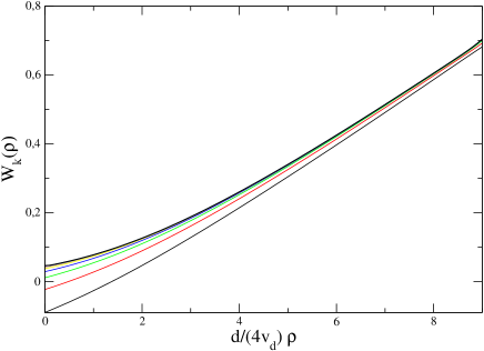
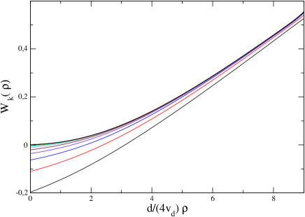
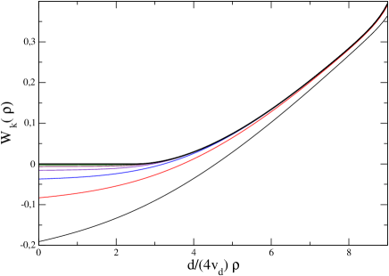
Figure 1: (color online) Top: typical evolution of the potential to the high temperature phase. Center: Typical evolution near the critical point. Bottom: Typical evolution of the potential in the low temperature phase.

There are also good news, as has been analyzed before Tetradis92 ; Tetradis95 . The first one is that in LPA and for some regulators, the singularity works as a barrier in flow equations and consequently the singularity is approached but never reached. Accordingly, the effective potential behaves as $W_{k}(\rho)\sim-k^{2}$ in all the internal region. This implies that in those cases, the LPA approximation preserves the convexity of the physical free-energy, that becomes flat in the internal region for $k\to 0$, as is shown in the bottom figure of Fig. 1. The second good news is that in the neighborhood of the singularity, the NPRG equation simplifies and analytical solutions can be obtained in that regime Tetradis92 . In this article following a suggestion made in Berges02 we exploit analytical solutions in the internal region of the potential in order to construct an efficient algorithm for the broken phase. It must be stressed that in order to do so, it has been necessary to improve considerably previous analytical results. In fact, previous results from Tetradis95 were only valid at small values of the fields but in order to implement the numerical scheme just mentioned it is necessary to know the analytical form of the solution for large values of $\rho$. Such solution is presented here for the LPA approximation and exploited in order to improve qualitatively the quality of the numerical treatment.

III Local Potential Approximation

The properties of NPRG equations in LPA approximation in the broken phase have already been analyzed in the literature both analytically and numerically Tetradis92 ; Tetradis95 ; Berges02 . In the present section we briefly review some of these works, generalize them to other cases and also show some limitations of previous results. After that we exploit the analytical results in order to implement a simple numerical analysis that is significantly more stable than previously considered .

The NPRG equation for the derivative of the effective potential for a generic regulator profile $R_{k}(q)$ reads Berges02 :

$$\partial_{t}W_{k}=-\frac{1}{2}\int\frac{d^{d}q}{(2\pi)^{d}} \partial_{t}R_{k}(q)\Big{\{}\frac{(N-1)W^{\prime}_{k}}{(q^{2}+R_{k}(q)+W_{k})^{2}}$$

$$+\frac{3W^{\prime}_{k}+2\rho W^{\prime\prime}_{k}}{(q^{2}+R_{k}(q)+W_{k}+2\rho W^{\prime}_{k})^{2}}\Big{\}}$$ (11)

Generalizing the discussion of the introduction, if the flow avoids the presence of singularities, one must have for all $\rho,\,q$ and $k$,

$$\left\{\begin{array}[]{l}q^{2}+R_{k}(q)+W_{k}>0,\\ q^{2}+R_{k}(q)+W_{k}+2\rho W^{\prime}_{k}>0\end{array}\right.$$ (12)

Now, in the internal region of the potential, one must have for any $k$, $W_{k}<0$. Accordingly, given that $R_{k}(q)\sim\mathcal{O}(k^{2})$, one concludes that, for $q\lesssim k$, $W_{k}(\rho)=\mathcal{O}(k^{2})$ (or smaller). On the other hand, in the low-temperature phase, the effective potential should have a non trivial behavior in terms of the physical dimensionful field, or equivalently in terms of $\rho$ . This motivates the use of $w_{k}(\rho)=W_{k}(\rho)/k^{2}$ instead of $W_{k}(\rho)$. It is convenient to introduce also the dimensionless function $r(y)$ defined by $R_{k}(q^{2})=q^{2}r(q^{2}/k^{2})$. With these definitions, the equation for $w_{k}(\rho)$ reads

$$\partial_{t}w_{k}=-2w_{k}+v_{d}k^{d-2}\int_{0}^{\infty}dy\,y^{d/2+1}\,r^{\prime}(y)$$

$$\times\Big{\{}\frac{(N-1)w^{\prime}_{k}}{(y(1+r(y))+w_{k})^{2}}+\frac{3w^{\prime}_{k}+2\rho w^{\prime\prime}_{k}}{(y(1+r(y))+w_{k}+2\rho w^{\prime}_{k})^{2}}\Big{\}}$$ (13)

This is in contrast with the usual set of variables used in studies of the critical domain, where $w_{k}$ is studied as a function of the dimensionless field which is, at LPA level, $\tilde{\rho}=\rho/k^{d-2}$.

In the rest of this section we study this equation for various values of $N$ and for various regulators both analytically and numerically. We show that the LPA equation does not avoid the existence of singularities of the flow unless a sufficiently strong regulator is included. In particular, the $\theta$-regulator (4) does respect this property. Smooth regulators respect this property also if $1+R^{\prime}(q=0)<0$ (corresponding to the case $\alpha>2$ for exponential regulators (5)) Tetradis92 ; Tetradis95 ; Berges02 . When this property is not fulfilled, the flow brings the potential to the singularity at $W_{k}+R(q)=0$ (typically at $\rho=0$ and $q=0$). This case was not fully addressed before in the literature even if such possibility was suggested in Tetradis95 ; Berges02 .

III.1 Large $N$

We first analyze the large $N$ limit of Eq. (III). This has been done long time ago Tetradis95 but we include it here for completeness. Moreover in this case many calculations can be done analytically and this motivates the general behavior of the potential obtained in the general case. The large $N$ limit is taken in the usual way (see, for example, D'Attanasio97 ). It is simpler to analyze it for the dimensionful derivative of the potential $W_{k}$. The coupling $u$ is of order $1/N$ and $V_{k}$ and $\rho$ are of order $N$. Accordingly, $W_{k}$ is of order $1$ and the large $N$ limit of Eq. (III) is:

$$\partial_{t}W_{k}=-\frac{N}{2}W^{\prime}_{k}\int\frac{d^{d}q}{(2\pi)^{d}}\frac{\partial_{t}R_{k}(q)}{(q^{2}+R_{k}(q)+W_{k})^{2}}$$ (14)

An implicit solution of this differential equation can be obtained by considering the inverse function $\rho=F_{k}(W)$ Tetradis95 . It satisfies $F_{k}^{\prime}(W)=1/W_{k}^{\prime}(\rho)$ and $\partial_{t}F_{k}(W)=-F_{k}^{\prime}(W)\partial_{t}W_{k}(\rho)$. Accordingly

$$\partial_{t}F_{k}(W)=\frac{N}{2}\int\frac{d^{d}q}{(2\pi)^{d}}\frac{\partial_{t}R_{k}(q)}{(q^{2}+R_{k}(q)+W)^{2}}$$ (15)

In this equation $W$ must be seen as an independent variable and consequently it can be integrated:

$$F_{k}(W)-F_{\Lambda}(W)=-\frac{N}{2}\int \frac{d^{d}q}{(2\pi)^{d}}\Big{\{}\frac{1}{q^{2}+R_{k}(q)+W}$$

$$-\frac{1}{q^{2}+R_{\Lambda}(q)+W}\Big{\}}$$ (16)

Given an initial condition for the potential, one can invert it in order to obtain $F_{\Lambda}(W)$. For example, for a Hamiltonian of the form (II), one obtains by inverting the relation between $W_{k}(\rho)$ and $\rho$:

$$F_{\Lambda}(W)=\frac{3}{u}(W-r)$$ (17)

If $\Lambda$ much larger than any other physical scale, one can absorb for $d<4$ the dependence on $\Lambda$ in a renormalization of the parameter $r$, obtaining an implicit equation for $W_{k}(\rho)$:

$$\rho -\frac{3}{u}(W_{k}(\rho)-\tilde{r})=-v_{d}Nk^{d-2}\int_{0}^{\infty}dy\,y^{d/2-1}$$

$$\times\Big{(}\frac{1}{y(1+r(y))+W_{k}(\rho)/k^{2}}-\frac{1}{y}\Big{)}.$$ (18)

where

$$\tilde{r}=r+\frac{Nu}{6}\int\frac{d^{d}q}{(2\pi)^{d}}\Big{\{}\frac{1}{q^{2}}-\frac{1}{q^{2}+R_{\Lambda}}\Big{\}}$$ (19)

is the renormalized mass parameter. We can see here that the minimum of the potential goes to zero when $k\to 0$ only if $\tilde{r}=0$. One deduces that $\tilde{r}\propto(T-T_{c})$ near the phase transition. We use this equation now in order to study the behavior for various regulators and, in particular, analyze how the convexity is approached in the low temperature phase and if and when the singularity can be reached at a non zero value of $k$. As expected, there is only a broken phase for $d>2$ because for $d\leq 2$ the integral in (19) is infrared divergent.

Let us consider now how this equation behaves for specific regulators. Let us consider first the $\theta$-regulator (4), that allows integrals to be done analytically at integer dimensions. For example, for $d=3$,

$$\Big{(} \frac{3}{u}(w_{k}k^{2}-\tilde{r})-\rho\Big{)}/(2v_{3}Nk)=$$

$$\left\{\begin{array}[]{ll}-1+\frac{1}{3+3w_{k}(\rho)}-\sqrt{w_{k}}\mathrm{arctan}(\sqrt{w_{k}})&\mathrm{if}\,w_{k}\geq 0\\ -1+\frac{1}{3+3w_{k}}+\sqrt{|w_{k}|}\mathrm{arctanh}(\sqrt{|w_{k}|})&\mathrm{if}\,w_{k}<0\end{array}\right.$$ (22)

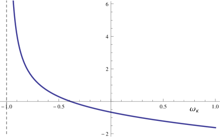
Figure 2: Right-hand-side of the equation (III.1) as function of $w_{k}$.

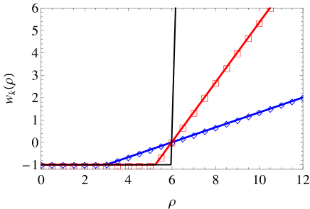
Figure 3: (color online) Solution of equation (III.1) for $w_{k}(\rho)$ as a function of $\rho$ for various values of $k=10^{-2}\Lambda$ (blue diamonds), $k=10^{-3}\Lambda$ (red squares), $10^{-4}\Lambda$ (black plain line).

Here we used as before the notation $w_{k}(\rho)=W_{k}(\rho)/k^{2}$. As for the flow equation (8), right hand side of (III.1) when $w_{k}(\rho)\to-1$. This implies that $w_{k}(\rho)=-1$ plays the role of a barrier and the solution never goes reaches it. In Fig.2, the right-hand-side of Eq. (III.1) is plotted as a function of $w_{k}$, and in Fig. 3 the numerical solution of the implicit Eq. (III.1) is shown for typical parameters in the low temperature phase. One observes that the singularity is approached by the solution in the internal region of the potential. Moreover, in Fig. 4, it can be seen that the singularity is approached but is not crossed. This is very similar to the results obtained in Berges02 except that it was not known that the $\theta-$regulator leads excatly to (III.1). In fact, the approach of the singularity can be discussed analytically. First of all, the right hand side of Eq. (III.1) is a monotonous decreasing function. Accordingly it is not difficult to convince oneself that a unique solution exists for any $\rho$ and $k$. This means that the singularity is never reached. Second, if the singularity is not crossed and a low temperature phase exists, there are values of $\rho$ with $w_{k}<0$ for all $k>0$. There are then only two possibilities. The first one, that corresponds either to $w_{k}\to 0^{-}$ or or to a negative constant larger than $-1$ in the internal region. However, if this were true, the right hand side of Eq. (III.1) would tend to a constant and the left hand side would tend to infinity when $k\to 0$ giving a contradiction. Correspondingly, the only remaining possibility is that $w_{k}(\rho)$ tend to $-1$ in all the internal region of the effective potential. Consequently, one can make an expansion of Eq. (III.1) in $\delta w_{k}(\rho)=w_{k}(\rho)+1$. At leading order one obtains:

$$\delta w_{k}(\rho)=\frac{2v_{3}N}{3}\frac{k}{-3\tilde{r}/u-\rho}$$ (23)

that, as observed before, leads to $\delta w_{k}(\rho)$ going to zero when $k\to 0$.

One can repeat this calculation for arbitrary integer dimension, but it is convenient to generalize it to an arbitrary $d$ by performing the expansion on $\delta w_{k}(\rho)$ directly at the level of flow equations. This allows the generalization of this procedure to arbitrary values of $N$. Before doing that, let us show the corresponding result for large values of $N$. If one expands at leading order on $\delta w_{k}(\rho)$ the flow equation (8) (taken at large $N$) one arrives at

$$\Big{(}\frac{1}{\delta w_{k}(\rho)}\Big{)}^{\prime}\sim-\frac{dk^{2-d}}{2v_{d}N}$$ (24)

whose solution is

$$\delta w_{k}(\rho)=\frac{2v_{d}Nk^{d-2}}{d}\frac{1}{\hat{\rho}_{0}(k)-\rho}.$$ (25)

Here $\hat{\rho}_{0}(k)$ is a integration constant that cannot be fixed without referring to the full (analytical or numerical) solution from the microscopic scale $\Lambda$ to the infrared limit ($k\to 0$). In the particular large $N$ case, this constant can be fixed analytically as in (23). In the $k\to 0$ limit, moreover, it must be identified with $\rho(k=0)$ because, as discussed before, in the entire internal zone of the potential, the approximation just analyzed becomes correct when $k\to 0$. From the solution of this equation we observe that the limit of validity of this approximation is precisely $\rho<\rho_{0}(k=0)$ when $k\to 0$. Another consequence of this general solution is that there is no broken phase in LPA for $d\leq 2$ (as expected from the Mermin-Wagner theorem). For $d\leq 2$, the “correction”, does not tend to zero, and the associated solution does not exist. Following the previous discussion, the only possibility, in absence of singularities is that at a given $k_{0}>0$, the minimum of the effective potential reaches $\rho=0$ and remains there after.

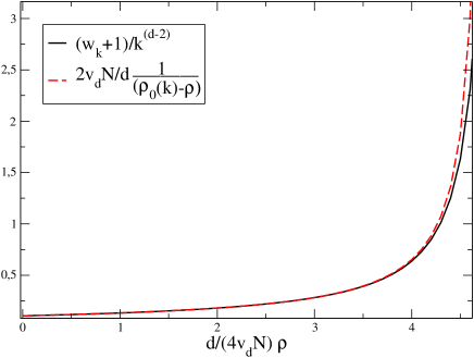
Figure 4: (color online) Comparison of numerical (black plain line) and semi-analytical (red dashed) solutions for $w_{k}+1$ at large $N$ as a function of $\rho$ for the $\theta$-regulator ($d=3$) for $k=0.002$.

The results from the numerical solution of (8) (taken at large $N$) coincides with the previous results. One can solve the equation with a standard finite differences explicit Euler procedure (with typical parameters $\Delta\rho=0.034$ and $\Delta t=-10^{-5}$ respectively). In Fig.4 the corresponding results are shown. Both solutions agree with good precision for values of $\rho$ for which $w_{k}(\rho)<0$. However, the singularity is approached and eventually the numerical code brings the potential to the wrong side of the singularity and the flow blows up. This is a purely numerical problem. In fact, by improving the parameters of the numerical code one can push the flow to smaller values of $k$. However, given that the singularity is approached rapidly it becomes impossible to go to really small values of $k$ by simply taking smaller grids and larger volumes in $\rho$. To solve this problem, we will present below an improved numerical algorithm that solves this difficulty.

The large-$N$ limit of the LPA equation (14) and its solution (III.1) has been partially analyzed previously for smooth regulators as the exponential one Tetradis92 ; Berges02 . In fact, there are essentially two typical cases (see Fig. 5): case (i) the inverse propagator $y(1+r(y))+W_{k}(\rho)/k^{2}$ has its minimum at a non zero value of $y$ (let us call it $y_{0}$), and case (ii) the inverse propagator has its minimum at $y=0$ with the derivative of the inverse propagator with respect to $y$ being positive at $y=0$. For the exponential regulator (5) the case (i) corresponds to the case $\alpha>2$ (i. e. for a strong enough regulator) and the case (ii) corresponds to the case $\alpha<2$. There is a third possible case that corresponds to a minimum of the inverse propagator at $y=0$, the derivative of which is zero. That is a very peculiar possibility that should be analyzed case-by-case.

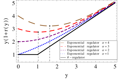
Figure 5: $y(1+r(y))$ for different regulators. The vertical dashed lines show the minimun of $y(1+r(y))$, $y_{0}$, for each case.

Let us discuss first case (i). It has been shown that in this case, the behavior of the flow in the low temperature phase is qualitatively similar to the one analyzed for the $\theta$-regulator Tetradis92 ; Berges02 : the singularity works as a barrier that is approached but never crossed and accordingly the convexity of the effective potential is ensured by the LPA equation. The exponent characterizing the approach to the singularity does not depend on the specific form of the regulator profile but is different to the particular case of the $\theta$-regulator. The right-hand side of Eq. (III.1) diverges when $W_{k}(\rho)/k^{2}$ approaches $-y_{0}(1+r(y_{0}))$. It is not hard to convince oneself that this singularity comes from the region of integration $y\approx y_{0}$. This can be seen in Fig 6 where the right hand side of Eq.(III.1) is represented in the case $\alpha=3$.

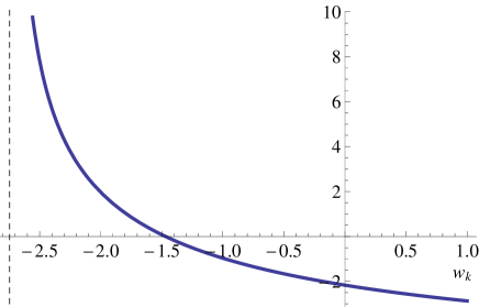
Figure 6: Right hand side of equation (III.1) for the exponential regulator and $\alpha=3$ ($d=3$). The dotted line point out the position of the singularity $-y_{0}(1+r(y_{0}))$.

Accordingly, one can obtain the equivalent of the integral when the singularity is approached by substituting in the numerator of the integral $y$ by $y_{0}$ and by expanding the denominator at leading non trivial order (at order $(y-y_{0})^{2}$). Eq. (III.1) near the singularity becomes:

$$\rho-\frac{3}{u}(W_{k}(\rho)-\tilde{r}) =-v_{d}Nk^{d-2}\int_{-\infty}^{\infty}\frac{dy\,y_{0}^{d/2-1}}{\delta w_{k}+C(y-y_{0})^{2}}$$

$$=-v_{d}Nk^{d-2}\frac{\pi\,y_{0}^{d/2-1}}{\sqrt{C\,\delta w_{k}}}$$ (26)

where the notations $\delta w_{k}=y_{0}(1+r(y_{0}))+W_{k}(\rho)/k^{2}$ and $C=r^{\prime}(y_{0})+y_{0}r^{\prime\prime}(y_{0})/2$ have been introduced. In this equation, the integration domain has been enlarged from $-\infty$ because this integration domain is regular in the limit $\delta w_{k}\to 0$. It is important to observe that the $(\delta w_{k})^{-1/2}$ behavior does not depend on the precise shape of the regulator as long as it has a regular behavior around $y_{0}$, the minimum at non zero value of $y$ and as long as $C$, the second derivative of the inverse propagator at $y_{0}$ is non-zero. This second hypothesis is not fulfilled by the $\theta$-regulator and this is why the right-hand-side of Eq. (III.1) has a different behavior. In fact, when $n-1$ derivatives of the inverse propagator with respect to $y$ are zero at $y_{0}$, the behavior of the right-hand-side of Eq. (III.1) is as $(\delta w_{k})^{-1+1/n}$, the $\theta$-regulator corresponding to the limit $n\to\infty$.

Eq. (III.1) can now be inverted by observing that, for the same reasons invoked for the $\theta$-regulator that, the singularity is approached but never reached. Accordingly when $k\to 0$, one can expand the Eq. (III.1) on $\delta w_{k}$. At leading order, one obtains:

$$\delta w_{k}(\rho)=\frac{1}{C}\Bigg{(}\frac{v_{d}Nk^{d-2}\pi y_{0}^{d/2-1}}{\rho_{0}-\rho}\Bigg{)}^{2}$$ (27)

with $\rho_{0}=-3\tilde{r}/u$. As done for the $\theta$-regulator, one can also obtain a similar expression by integrating directly the flow equation (14). One obtains the same expression, except that $\rho_{0}$ is replaced by an arbitrary function of $k$, $\hat{\rho}_{0}(k)$ that comes as an integration constant (independent of $\rho$). As before, in the limit $k\to 0$, $\hat{\rho}_{0}(k)$ can be interpreted as the position of the minimum of the effective potential $\rho_{0}(k=0)$.

We display in Fig. 7 a numerical solution of the LPA equation in the large $N$ limit (14) that has been, as before, using finite differences and explicit Euler method with typical parameters $\Delta\rho=0.034$ and $\Delta t=-10^{-5}$ respectively. It must be stressed that to observe numerically the proper behavior of the solution in the internal region of the potential is much more numerically demanding than, for example, to study of the critical behavior of these models (in that case one can typically obtain stable results with $\Delta\rho/k^{d-2}=0.1$ and $\Delta t=-2.10^{-3}$). The only difference with the $\theta-$regulator is that the integrals over momenta must be done numerically. We employ for this purpose Simpson’s rule with a regular grid in momenta with 80 steps of a dimensionless momentum step of 0.1. The solution agrees with the analytical behavior just presented. However, as with the $\theta$-regulator, at a certain value of $k$, the singularity is crossed due to numerical lack of precision and consequently the flow collapses. As with the $\theta$-regulator, we present below a more elaborated method in order to avoid such collapse.

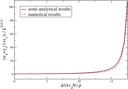
Figure 7: (color online) Comparison of numerical (black plain line) and semi-analytical (red dashed) solutions at large $N$ for $w_{k}+y_{0}(1+r(y_{0}))$ as a function of $\rho$ for the exponential regulator ($d=3$). Curves for $k=0.08$.

Let us now consider the case (ii) (corresponding to $\alpha<2$ in the particular case of the exponential regulator). In this case, the singularity does not work any more as a barrier and the integral remains bounded when the singularity is approached. The singularity in that case shows up first at $y=0$, and corresponds to the point where $w_{k}(\rho)$ approaches $-\tilde{R}\equiv-\lim_{y\to 0}y(1+r(y))$. The integral is not differentiable at $w_{k}(\rho)=-\tilde{R}$ but remains continuous at this point. In the particular case of the expontial regulator (5), $\tilde{R}=\alpha$. As mentioned before, the flow blows up at a finite scale $k_{0}$ because $U_{k}$ hits the singularity at$k=k_{0}$. This singularity that occurs at finite $k$ is also observed when numerically integrating the flow equation. However, this is not very conclusive because when $\alpha>2$, the singularity that should not be reached in principle is actually reached because of numerical inaccuracies. However, in order to be fully convinced that the singularity is hit, one can exploit the implicit large $N$ solution (III.1) and observe that there is a solution for $w_{k}=-\tilde{R}$ when $\rho$ and $k$ are small enough. In order to see that, one can observe that the right-hand-side of equation (III.1) is bounded from above as a function of $w_{k}$. As an example, in Fig. 8, the case $\alpha=1$ is represented. One sees that the right-hand-side presents a singularity but that it is finite, not diverging. As a consquence, nothing forbids the large $N$ implicit solution (III.1) to reach the singularity at $k>0$.

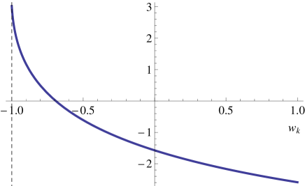
Figure 8: Right hand side of equation (III.1) for the exponential regulator and $\alpha=1$ ($d=3$). The dotted line point out the position of the singularity $-\tilde{R}=-\lim_{y\to 0}y(1+r(y))$

Having discussed the standard numerical solution of the equation, the implicit analytical solution and the explicit analytical solution near the singularity, we present now an improved numerical solution that exploits the obtained analytical behavior in the two cases discussed above where the singularity is avoided: the $\theta$-regulator and the smooth regulator in case (i). The idea is simple and has been already suggested (but not implemented) in Berges02 . One can employ a standard numerical procedure at typical points in a grid, but in a region where the solution is close enough to the singularity (and where the analytical solutions (25) or (27) are therefore justified), one replaces the result of the flow equation by the analytical expressions (25) or (27), depending on the chosen regulator. For a given smooth regulator, the constant $y_{0}$ can be calculated (by looking at the minimum of $y(1+r(y))$). For values of $\rho$ at which $w_{k}$ is above a chosen threshold, one implement a standard numerical solution (finite differences plus explicit Euler). The value of the integration constant $\hat{\rho}_{0}(k)$ is taken in order to require the continuity between the analytical solution below the threshold and the purely numerical one above it. It must be stressed that this algorithm requires the knowledge of the solution in the full internal region and not only around $\rho=0$ as was obtained in Tetradis92 ; Tetradis95 . For actual numerical implementations with the $\theta$-regulator we took the value for the threshold at $w_{k}=-0.98$. In the case of the the exponential regulator, we chose $\alpha=3$ (for which $y_{0}\simeq 1.035658$) and we chose the threshold value $w_{k}=-2.74$. This numerical procedure is completely stable. The flow can be continued down to $k/\Lambda\sim 1.5\times 10^{-8}$ without encountering any difficulty. From the result of $w_{k}$ one can reconstruct the dimensionful potential which, as expected, is convex. The corresponding result is shown in Fig.9.

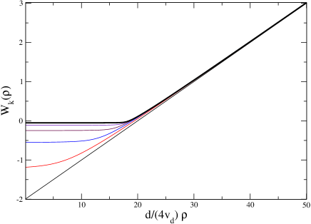
Figure 9: Derivative of the potential at large $N$ and $d=3$ as a function of $\rho$ for various values of $k$ (lower curves are for larger values of $k$).

The large $N$ limit is not particularly exciting because the flow equation can be essentially solved analytically and because physically interesting models correspond to lower values of $N$. We merely use it to test various ideas about the approach to convexity. In the following we exploit such ideas to more realistic values of $N$, beginning with the $N=1$ and finally generalizing to other values of $N$.

III.2 Finite $N$

We analyze now the the finite $N$ case, where no (even implicit) analytical solution is known. As done for large $N$ we consider the corresponding equations (8) and (III) both analytically and numerically, first with the $\theta$-regulator and then for a generic smooth regulator (the corresponding numerical implementation is performed for the exponential one).

Consider first the LPA flow equation with the $\theta$-regulator for $N=1$:

$$\partial_{t}w_{k}=-2w_{k}-\frac{4v_{d}}{d}k^{d-2}\frac{3w_{k}^{\prime}+2\rho w_{k}^{\prime\prime}}{(1+w_{k}+2\rho w_{k}^{\prime})^{2}}$$ (28)

Again, let us admit (as clearly seen in the numerical solution of the equation in $d=3$) that the LPA equation displays a low temperature phase in which there is a minimum of the potential $\rho_{0}(k)$ with $w_{k}(\rho_{0}(k))=W_{k}(\rho_{0}(k))/k^{2}=0$ for any $k>0$ and with $\rho_{0}(k=0)>0$. Repeating a similar analysis to the one performed for large $N$, one concludes that the flow approaches the singularity where $1+w_{k}(\rho)+2\rho w^{\prime}_{k}(\rho)=0$. In that case, there are, again two possibilities: either the singularity is never reached or it is crossed.

It is difficult to give a general analytical proof for finite $N$ that the singularity is not crossed at any finite value of $k$, but the numerical solution of the equations gives clear indications in this direction for the $\theta-$regulator. Under this hypothesis, one concludes that when $k$ is small enough the flow approaches a regime when $1+w_{k}(\rho)+2\rho w^{\prime}_{k}(\rho)$ is small in all the internal region of the potential but positive. Moreover, in absence of singularities for $k>0$, $w_{k}(\rho)$ is a regular function of $\rho$. The solution of the equation $1+w_{k}(\rho)+2\rho w^{\prime}_{k}(\rho)\approx 0$ is

$$w_{k}(\rho)\approx-1+A_{k}/\sqrt{\rho},$$ (29)

where $A_{k}$ is an arbitrary function of $k$. However, the solution being regular for any $\rho$ and, in particular for $\rho=0$, one concludes that $1+w_{k}(\rho)+2\rho w^{\prime}_{k}(\rho)\approx 0$ is equivalent to $1+w_{k}(\rho)\approx 0$ in the entire internal region of the potential. This is the same behavior as for large $N$ but for a slightly subtler reason. Moreover, as when $N$ is large, one can analyze the approach to this regime by expanding Eq. (28) in $\delta w_{k}(\rho)=w_{k}(\rho)+1$:

$$\frac{4v_{d}}{d}k^{d-2}\frac{3\delta w_{k}^{\prime}+2\rho\delta w_{k}^{\prime\prime}}{(\delta w_{k}+2\rho\delta w_{k}^{\prime})^{2}}=2+\mathcal{O}(\delta w_{k})$$ (30)

Neglecting the term $\mathcal{O}(\delta w_{k})$ in the right hand side, one can solve the Eq. (30). The solutions that are regular at $\rho\sim 0$ are of the form

$$\delta w_{k}(\rho)=\frac{v_{d}}{d}\frac{k^{d-2}}{\sqrt{\rho_{0}(k)\rho}}\log\Bigg{(}\frac{\sqrt{\rho_{0}(k)}+\sqrt{\rho}}{\sqrt{\rho_{0}(k)}-\sqrt{\rho}}\Bigg{)}$$ (31)

where $\rho_{0}(k)$ is an arbitrary function depending on the initial conditions of the flow. Given that this solution is only valid for small values of $k$, a possible $k$ dependence of $\rho_{0}$ can be neglected. It is in the $k\to 0$ limit the position of the minimum of the effective potential.

For generic values of $N$, the LPA equation with the $\theta$-regulator is:

$$\partial_{t}w_{k}=-2w_{k}-\frac{4v_{d}}{d}k^{d-2}\Bigg{(}\frac{3w_{k}^{\prime}+2\rho w_{k}^{\prime\prime}}{(1+w_{k}+2\rho w_{k}^{\prime})^{2}}+\frac{(N-1)w_{k}^{\prime}}{(1+w_{k})^{2}}\Bigg{)}$$ (32)

The two convexity conditions to be fulfilled are those of large $N$ and of $N=1$. As explained before, and admitting that both singularities are not crossed at finite $k$, both of them imply that when $k$ is small, $\delta w_{k}(\rho)=w_{k}(\rho)+1\ll 1$. As in previous cases, one can expand the equation (32) in $\delta w_{k}$ yielding the differential equation

$$\rho_{0}(k)-\rho=\frac{2v_{d}}{d}k^{d-2}\Bigg{(}\frac{1}{\delta w_{k}+2\rho\delta w_{k}^{\prime}}+\frac{N-1}{\delta w_{k}}\Bigg{)}$$ (33)

where $\rho_{0}(k)$ is an arbitrary function depending on initial conditions. As before, $\rho_{0}(k)$ can be interpreted when $k\to 0$ as the position of the minimum for the potential, and one can neglect its $k$ dependence. Eq. (33) cannot be solved analytically except for the previously considered cases ($N=1$ and large $N$ ). Being a differential equation one could expect that for any $\rho_{0}$ it has an infinite number of solutions corresponding to different choices of $\delta w_{k}(\rho=0)$. However, as before, one must require that it is well-behaved in all the domain of validity of the approximation, and in particular for $\rho=0$. This fixes the value of $\delta w_{k}(\rho=0)$ in terms of $\rho_{0}$:

$$\delta w_{k}(\rho=0)=\frac{2v_{d}}{d}k^{d-2}\frac{N}{\rho_{0}(k)}$$ (34)

yielding a single regular solution in the domain of validity of the equation. The Eq. (33) can be solved numerically easily. It is convenient to define

$$u =\frac{\rho}{\rho_{0}(k)}$$

$$f(u) =\frac{\delta w_{k}(\rho)}{\delta w_{k}(\rho=0)}$$ (35)

that yields the following equation for $f(u)$:

$$1-u=\frac{1}{N}\Bigg{(}\frac{1}{f(u)+2uf^{\prime}(u)}+\frac{N-1}{f(u)}\Bigg{)}$$ (36)

with the initial condition $f(u=0)=1$. The expression of $\delta w_{k}(\rho)$ can be reconstructed from that of $f(u)$ obtained at a given $N$ and for an arbitrary $\rho_{0}(k)$:

$$\delta w_{k}(\rho)=\frac{2v_{d}}{d}k^{d-2}\frac{N}{\rho_{0}(k)}f(\rho/\rho_{0}(k))$$ (37)

The form of $f(u)$ for various values of $N$ obtained by numerically solving the Eq. (36) are shown in Fig.10. It must be stressed that the correction to $\delta w_{k}\approx 0$ differs fromt its large $N$ limit. However, for any $N$ one generically approaches the regime where $\delta w_{k}\approx 0$ but the corresponding function $f(u)$ depends on $N$ for generic values of $\rho$ in the internal region. This is in contrast to the $\rho\to 0$ limit where it has been shown Tetradis92 ; Tetradis95 that the large $N$ form is self-consistent for any $N$.

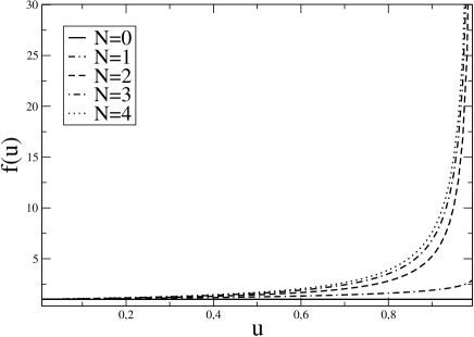
Figure 10: $f(u)$ as a function of $u$ for various values of $N$.

We also solve numerically the LPA equation with the $\theta$-regulator for various values of $N$ with the same procedure presented before for large $N$. First, we solve it directly using finite-differences for the derivatives and an explicit Euler algorithm for the evolution in $t$. Typically the parameters used are $\Delta\tilde{\rho}=0.1$ and $\Delta t=-10^{-5}$. As can be seen in Fig. 11, in all cases (including $N=0$), a low temperature phase is found for $d>2$ and the numerical solution indicates that the function $w_{k}(\rho)$ approaches (without crossing) $-1$ in all the internal region of the potential. However, like for large $N$, when the solution is too close to the singularity it may happen that discretization errors leads to an artificial crossing of the singularity.

It is interesting to note that the numerical implementation of the LPA equation for $N=1$ turns out to be much more difficult than for $N>1$. The reason for this, at first sight surprising, result is two-fold. First, as explained before, for $N>1$ the convexity condition $w_{k}(\rho)>-1$ is imposed directly by the term of the LPA Eq. (III) proportional to $N-1$. The other term of the right-hand-side of the equation (the only present when $N=1$), imposes the weaker constraint $w_{k}(\rho)+2\rho w_{k}^{\prime}(\rho)>-1$ that eventually leads to the same consequence ($w_{k}(\rho)>-1$) but in a much more indirect way (see above). Numerically this effect seems to be harder to control. The second reason is that, for $N=1$, the dimensionful physical effective potential $U_{k=0}$ has a discontinuity in its second derivative at the minimum of the potential. This is simply related to the fact that for $N=1$ the susceptibility is finite both in the high and low temperature phase (only diverging asymptotically when the critical temperature is approached). On the contrary, the second derivative of the physical effective potential is continuous for $N>1$, even at the minimum. This expresses the fact that the susceptibility of the $O(N)$ models with continuous symmetries ($N>1$) is infinite for any temperature below the critical one because of Goldstone modes. In practice, the effective potential for $k>0$ remains much more regular around the minimum for $N>1$ diminishing the sources of instabilities.

In order to improve the stability of the numerical solution, we employed the same procedure presented above for large $N$: we fixed a threshold $w^{\text{threshold}}=-0.95$, solved numerically the flow equation (III) when $w_{k}(\rho)$ is above $w^{\text{threshold}}$ and imposed the quasi-analytical form given by Eq. (37) for $w<w^{\text{threshold}}$. The implementation of this procedure proves to be essentially stable at arbitrary values of $t$ for all $N>1$. A typical example of a such solution is shown Fig.11. As before, the numerical solution of Eq.(III) for $N=1$ is much more demanding. In fact, the procedure explained above does not work for $N=1$ as efficiently as in the $N>1$ case, although (30) is again a good approximation in all the internal region of the potential. It turns out that the mismatch between the second derivatives of the potential at the matching point corresponding to $w^{\text{threshold}}$ is large enough to generate numerical instabilities.

$\begin{array}[]{cc}\includegraphics[width=227.62204pt]{10-eps-converted-to.pdf}\end{array}$

Figure 11: (color online) $w_{k}(\rho=0)$ as a function of $t=\log(k/\Lambda)$ for $N=4$ and $d=3$. Comparison between the direct numerical solution (red circles) and the improved algorithm (black plain line) in both cases with the $\theta-$regulator.

We analyzed the equation also for typical smooth regulators. Again, there are two different cases, depending on the position of the minimum of $y(1+r(y))$. As for large $N$, when the minimum takes place at a $y=y_{0}>0$, integrals in the right-hand-side of the LPA equation can be approximated as in (III.1). Accordingly the singularities play the role of a barrier that cannot be crossed and one arrives at a scenario very similar to the one of the $\theta$-regulator: the singularity is approached but never crossed. In this case the behavior of the analytical solution when $k\to 0$ is

$$\delta w_{k}\sim k^{2(d-2)}f(\rho).$$ (38)

For for $N=1$ the function $f(\rho)$ can be found analytically:

$$f(\rho)=\frac{1}{C^{2}}\Bigg{(}\frac{1}{\rho_{0}^{3/2}\sqrt{\rho}}\log\Big{(}\frac{\sqrt{\rho}+\sqrt{\rho_{0}}}{\sqrt{\rho_{0}}-\sqrt{\rho}}\Big{)}+\frac{2}{\rho_{0}(\rho_{0}-\rho)}\Bigg{)}$$

and for $N>1$ it can be obtained by solving the differential equation:

$$f+2\rho f^{\prime}=\frac{1}{\Big{(}\frac{C}{2}(\rho_{0}-\rho)-\frac{N-1}{\sqrt{f}}\Big{)}^{2}}.$$

In both cases the constant $C$ is related to the minimum as

$$C=\frac{y_{0}(1+r(y_{0}))}{v_{d}y_{0}^{d/2}r(y_{0})\pi}\sqrt{r^{\prime}(y_{0})+y_{0}r^{\prime\prime}(y_{0})/2}.$$

Following the same procedure we can go further in the solution of the flow equation as it is shown in the Fig.12.

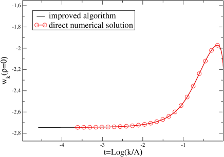
Figure 12: (color online) Comparison between the direct numerical solution (red circles) and the improved algorithm (black plain line). $N=4$ and $d=3$ using the exponential regulator with $\alpha=3$.

Having discussed the treatment of the LPA equation in the various cases and showing a new numerical algorithm that is much more stable than the standard one for all $N>1$, we consider now the next-to-leading order of the derivative expansion.

IV Derivative Expansion at order $\mathcal{O}(\partial^{2})$

In this section, we generalize the previous numerical studies on the approach to a convex free-energy at the LPA level to second order in the derivative expansion. This approximation corresponds to an expansion to second order of the NPRG equation in powers of the external momenta, see Eq. (II). We derived the corresponding NPRG equations and we verified the equivalence with VonGersdorff:2000kp . We limit ourselves to a direct numerical analysis leaving for the future an analytical study analogous to the one performed for the LPA. This analysis should again improve the numerical integration of the flow equations but the number of cases to be studied brings it clearly beyond the scope of the present article. One aspect that cannot be addressed at the LPA level is the broken phase for $N=1$ in $d=2$ since the running of the field renormalization factor is neglected which artificially destroys the broken phase. On the contrary, at order $O(\partial^{2})$ of the DE, a phase transition is found at finite temperature for $N=1$ in $d=2$ VonGersdorff:2000kp ; Jakubczyk:2014isa . For $N>2$, no phase transition is found with this approximation in agreement with the Mermin-Wagner theorem and for $N=2$, the Kosterlitz-Thouless phase transition is correctly described Kosterlitz:1973xp .

An important difference between the order $O(\partial^{2})$ of the DE and the LPA is that it is convenient to introduce a pre-factor in the regulator function $R_{k}(q)$ that evolves with $k$ (as usually done in the study of the critical regime). This pre-factor has many purposes in the critical regime. In the present case let us consider the inverse propagator, (for $N=1$ for example):

$$G_{k}^{-1}(q)=q^{2}Z_{k}(\rho)+W_{k}(\rho)+2\rho W^{\prime}_{k}(\rho)+R_{k}(q).$$ (39)

For $R_{k}(q)$ to regulate efficiently and for all values of $k$ the small wave-number modes, it is necessary that it is at least of of the same order as $q^{2}Z_{k}(\rho)$ up to $q\sim k$. As usual, we use regulators of the form

$$R_{k}(q)=Z_{k}\hat{R}_{k}(q)$$ (40)

where $\hat{R}_{k}(q)$ are the regulator profiles used at the LPA level, see Eqs. (4,5), and $Z_{k}$ is fixed as $Z_{k}(\rho)$ at a particular value of $\rho$. The difficulty is that $Z_{k}(\rho)$ depends strongly on $\rho$ and, not surprisingly, the behavior of this function for $\rho$ larger or smaller than the minimum of the potential is very different in the low temperature phase when $k\to 0$. We analyze two possible choices: $\rho$ larger or smaller than $\rho_{0}$, the minimum of the potential when $k\to 0$. As we will see, the appropriate choice for this point depends on the value of $N$. On one hand, when $N>1$, we observe that the flow is more stable if $Z_{k}$ is taken as the value of $Z_{k}(\rho)$ for a $\rho>\rho_{0}$, in some cases in a very significant way. For this reason, for those values of $N$, all results presented below correspond to this choice of $\rho$ (more precisely, $\rho=2\rho_{0}$). On the other hand, for $N=1$, one must fix the value of $Z_{k}$ for a $\rho$ in the “internal” part of the potential, as explained below. If this is not done, the flow of the potential hits the singularity as with the LPA for a regulator not strong enough. As for the choice of the regulator profile, the main advantage of the $\theta$-regulator (4) is lost at the second order of the DE because the integrals cannot be performed any more analytically. We therefore use the exponential regulator (5) in what follows and we choose a prefactor $\alpha$ larger than 2 to avoid singularities in the flow, see section III.

The large $N$ case is not particularly useful for the second order of the derivative expansion, because in that limit, the LPA equation for the potential becomes exact. We consider then, first, the single scalar case, generalizing those results to the $O(N)$ case after. An analysis of such theories has been done a few years ago at the second order of the derivative expansion in Zappala12 but for $d=4$. Here we consider dimensions $d<4$ that are generically much richer for scalar theories. Moreover, an interesting but very weak logarithmic divergence of the function $Z(\rho)+\rho Y(\rho)$ were observed in Zappala12 . In $d<4$, we observe clearer and stronger effects because the corresponding divergences is power-law, as will be discussed below.

IV.1 Single scalar case

As said before, in the $N=1$ case, one can simply take $Y_{k}=0$. As seen in figure 13, when the renormalization factor $Z_{k}$ in the regulator profile is chosen for values of $\rho$ in the “external” part of the effective potential, the flow collapses after a certain renormalization-group “time”. When $\rho_{textren}>\rho_{0}$, the flow blows at a finite RG time because there is no barrier preventing the singularity to be reached. The reasons are the following, i) In the external part, the function $Z_{k}(\rho)$ rapidly stabilizes and accordingly the function $Z_{k}$ becomes a constant below a finite value of $k$, ii) The flow of $Z_{k}(\rho)$ in the “internal” part continues to grow without bound, iii) For all $k>0$ in the internal part the potential is not convex. Accordingly, the regulator becomes negligible in the internal part of the potential and the flattening of the internal part is not strong enough to avoid the singularity (as is the case for the LPA with an exponential regulator with $\alpha<2$). For $N=1$ we therefore choose $Z_{k}$ as the value of $Z_{k}(\rho)$ at $\rho=0$.

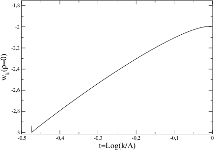
Figure 13: $w_{k}(\rho=0)$ as a function of $t=\log(k/\Lambda)$ for $N=1$ and $d=3$ using the exponential regulator (5) with $\alpha=3$. Normalization fixed at $\rho=2\rho_{0}$.

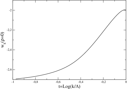
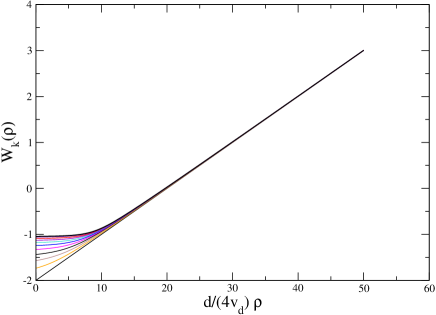
Figure 14: (Top) $w_{k}(\rho=0)$ as a function of $t=\log(k/\Lambda)$. (Bottom, color online) $W_{k}(\rho)$ as a function of $\rho$ for various values of $t$. In both figures, $N=1$ and $d=3$ using the exponential regulator (5) with $\alpha=3$ and normalization fixed at $\rho=0$.

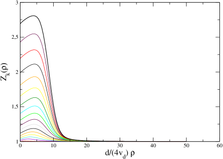
Figure 15: (color online) $Z_{k}(\rho)$ for $N=1$ and $d=3$ using the exponential regulator (5) with $\alpha=3$. Normalization fixed at $\rho=0$.

With this choice, we observe as in the LPA case that the effective potential runs in the low temperature phase to a convex potential that is flat in the “internal” part but that finally collapses when, due to numerical lack of precision, the singularity of the flow equation is crossed. We observe systematically that if the discretization parameters of the program are improved, the instability appears at larger renormalization-group “times” (indicating that this phenomenon is a numerical artifact), but, in practice, they are finally reached. A typical run of the effective potential and of the function $Z_{k}(\rho)$ is shown in Figs. 14 and 15 for $d=3$. In all cases, we observe, on the top of a potential approaching the convexity, a function $Z_{k}(\rho)$ that seems to diverge when $k\to 0$ for values of $\rho$ in the “internal” part of the potential. In order to study how this divergence takes place, we plot in Fig. 16 the quantity $\eta_{k}=-\partial_{t}\log Z_{k}$ that shows the exponent of the divergence of $Z_{k}(\rho=0)$ as a function of $t$. We observe that the exponent seems to stabilize at values $\sim 1.5$ but at that value of $t$ the singularity is hit and the flow breaks down. In Fig. 17 the renormalized function

$$\hat{Z}_{k}(\rho)=\frac{Z_{k}(\rho)}{Z_{k}(\rho=0)}$$ (41)

is plotted. It seems to approach a finite limit for values of $\rho$ corresponding to the “internal” part of the potential and, as expected, to tend to zero in the “external” part (given the fact that the function $Z_{k}(\rho)$ seems to go to a finite limit in that regime). As a conclusion, the second order of the DE seems to respect be able to mantain the convexity property and the singularity present in the flow equation for the potencial does not seem to be hit. However, a standard numerical implementation finally breaks down (as in the LPA) because of the unavoidable lack of precision.

Figure 16: $\eta_{k}$ for $N=1$ and $d=3$ using the exponential regulator (5) with $\alpha=3$. Normalization fixed at $\rho=0$. Observe that, given that $Z_{k}(\rho=0)$ and $Z_{k}(\rho=2\rho_{0})$ are different, the position of the singularity is different from the LPA order.

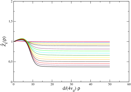
Figure 17: (color online) $\hat{Z}_{k}(\rho)$ as function of $\rho$ for various values of $t$ for $N=1$ and $d=3$ using the exponential regulator (5) with $\alpha=3$. Normalization fixed at $\rho=0$.

As said before, contrarily to what happens at the LPA level, the second order of the DE clearly shows for the single scalar case a low temperature phase not only in $d=3$ but also in $d=2$. This is shown in Figs.  18,19 and 20. As explained before, this is one of the most important ingredients absent at the LPA level and one of the main reasons to go beyond. The results for $d=2$ seem to be qualitatively similar to those of $d=3$ for $N=1$.

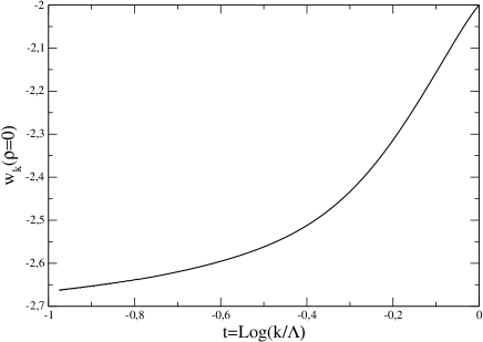
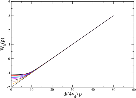
Figure 18: (Top) $w_{k}(\rho=0)$ as a function of $t=\log(k/\Lambda)$. (Bottom, color online) $W_{k}(\rho)$ as a function of $\rho$ for different values of $t$. In both figures, for $N=1$ and $d=2$ using the exponential regulator (5) with $\alpha=3$ and normalization fixed at $\rho=0$.

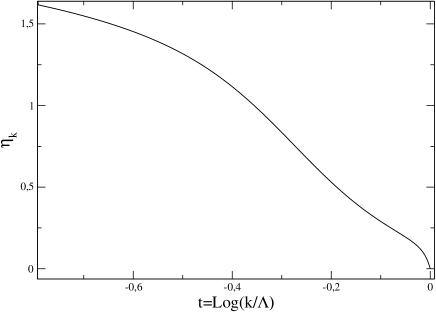
Figure 19: $\eta_{k}$ for $N=1$ and $d=2$ using the exponential regulator (5) with $\alpha=3$. Normalization fixed at $\rho=0$.

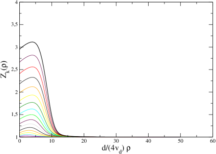
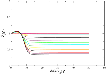
Figure 20: (Top, color online) $Z_{k}(\rho)$ as a function of $\rho$. (Bottom, color online) $\hat{Z}_{k}(\rho)$ as function of $\rho$. In both cases, for various values of $t$ for $N=1$ and $d=2$ using the exponential regulator (5) with $\alpha=3$. Normalization fixed at $\rho=0$.

IV.2 Generic $O(N)$ model

In this section we extend the analysis of the second order of the derivative expansion in the low temperature phase for $N>1$.

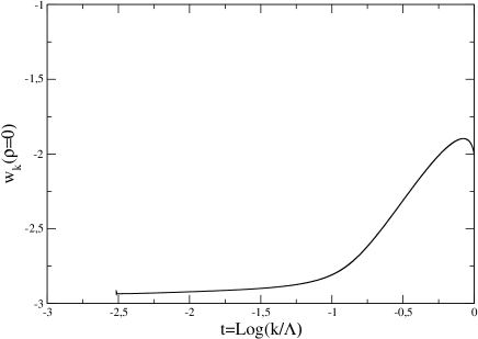
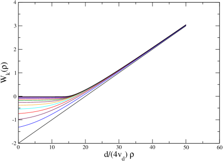
Figure 21: (Top) $w_{k}(\rho=0)$ as a function of $t=\log(k/\Lambda)$. (Bottom, color online) $W_{k}(\rho)$ as a function of $\rho$ for various values of $t$. In both figures, for $N=4$ and $d=3$ using the exponential regulator (5) with $\alpha=3$ and normalization fixed at $\rho=2\rho_{0}$.

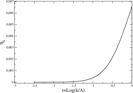
Figure 22: $\eta_{k}$ as a function of $t$ for $N=4$ and $d=3$ using the exponential regulator (5) with $\alpha=3$. Normalization fixed at $\rho=2\rho_{0}$.

In this case, in contrast to the $N=1$ case, choosing $Z_{k}$ at values larger than $\rho_{0}$ turns out to give a more stable flow than the one obtained if $Z_{k}$ is fixed at $\rho$ smaller than $\rho_{0}$. When $Z_{k}$ is fixed at values larger than $\rho_{0}$ the flow does not explode until large values of $|t|$. Fig.21 shows that, as for LPA, a convex potential is approached along the flow. As before, we need to choose a value of $\alpha$ larger than $2$ to avoid hitting the singularity. We employed an Euler algorithm of the same kind that the one employed in the LPA (without the improvement in the internal part of the potential). Even if convexity is clearly visible we are not able to reach very large values of $|t|$, because of the same numerical instabilities discussed before. In any case, as for the LPA approximation, the flow for $N>1$ is much more stable than for the $N=1$. It is very plausible that an hybrid algorithm that exploits the exact behavior of NPRG equations in the internal region would, as for the LPA case, allow to make the flow even more stable.

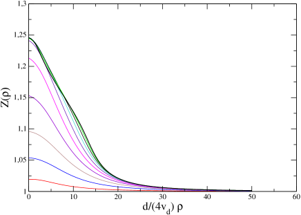
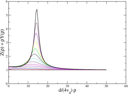
Figure 23: (Top, color online) $Z_{k}(\rho)$ as a function of $\rho$. (Bottom, color online) $Z_{k}(\rho)+\rho Y_{k}(\rho)$ as function of $\rho$. In both cases, for various values of $t$ for $N=4$ and $d=3$ using the exponential regulator (5) with $\alpha=3$. Normalization fixed at $\rho=2\rho_{0}$.

It is interesting to discuss also the results for the flows of the functions $Z_{k}(\rho)$ and $Y_{k}(\rho)$. In fact, we prefer to present the results in terms of the transverse renormalization function $Z_{k}(\rho)$ and the longitudinal one, $Z_{k}(\rho)+\rho Y_{k}(\rho)$, as shown in Figs. 22 and 23. As one can observe, the function $Z_{k}(\rho)$ seems to reach a limit when $k\to 0$. In contrast, the longitudinal renormalization factor $Z_{k}(\rho)+\rho Y_{k}(\rho)$ seems to grow without bound around the minimum of the potential. This is similar to what is observed in $d=4$ in Zappala12 . However, in the $d=3$ the effect is much stronger. In what concerns the behavior of these functions in the “external” region of the potential, it seems to stabilize faster. This can be seen in the running of the anomalous dimension (fixed via the value of $Z_{k}$ at $2\rho_{0}$) as can be seen in Fig. 22. One observes that $\eta_{k}$ goes to zero as expected in the low temperature phase.

We have thus managed to study the low temperature phase of $O(N)$ models in the second order of the DE and shown that if an appropriate regulator and renormalization condition is used, one can show clearly that the property of convexity of the effective potential is respected. The flow finally becomes unstable for numerical reasons. When $N>1$ the flow is much more stable than in the single scalar case $N=1$.

V Conclusions

In the present article we analyze the NPRG equations both at the leading order (LPA) of the Derivative Expansion and at next-to-leading order (order $\mathcal{\partial}^{2}$) in the low temperature phase. These simple approximations performed at the level of NPRG equations are able, in contrast with most perturbative schemes, to preserve the convexity of the free energy. In the present article we show that this is only true for certain regulators. In particular, the most used regulators used (the $\theta$-regulator and the exponential regulator) are able to respect the convexity of the free energy. However, in the case of the exponential regulator, it is necessary to choose a large enough pre-factor. If this is not done, a singularity of the flow is hit.

Even if an appropriate regulator is chosen, there is a practical difficulty: the flow approaches a singularity without crossing it. As a consequence, even if the singularity is never hit, the flow becomes numerically unstable for low enough values of $k$. In order to deal with this problem many algorithms have been proposed in the literature. We implement at the LPA level a very simple algorithm that exploits the exact behavior of the flow in the “internal” part of the potential and that makes the flow stable for essentially arbitrary values of $k$ when $N>1$. The $N=1$ case turns out to be much more challenging for various reasons discussed along the article. The most important one comes from the fact that the physical longitudinal susceptibility is a continuous function of the external field for $N>1$ but has a discontinuity for $N=1$ when $k\to 0$. This makes this case much harder to treat. We obtain for $N>1$ and with a very simple algorithm a flow that is qualitatively more stable than what was obtained before.

On top of this analysis, we studied the behavior of the flow in the low temperature phase at order $\mathcal{\partial}^{2}$ of the Derivative Expansion. We observe that in order to approach a convex free-energy it is necessary to normalize the field in a different way in the case $N=1$ and in the case $N>1$. On one hand, in order to avoid reaching the singularity of the flow for $N=1$ it is necessary to normalize the field in the “internal” region of the potential. On the other hand, in the $N>1$ case it is necessary to normalize the field in the “external” part of the potential. Once these choices are made and an appropriate regulator is chosen, the flow approaches a convex free-energy. Of course, in practice, the flow becomes numerically unstable when $k$ is very small and the singularity is reached in practice.

For the future, we are planing to implement the same kind of algorithm that we presented in the LPA case at second order of the Derivative Expansion $\mathcal{O}(\partial^{2})$. We are planing also to make the same kind of analysis in more elaborated approximations such as the one proposed in Blaizot05 ; Benitez09 ; Benitez12 . We would like also to try to implement an improved algorithm in these kinds of approximations also. These improved approximations and algorithms in the low temperature phase of $O(N)$ models could be useful in the analysis of a large variety of physical problems, that we are planing to analyze, as the formation of bound states or the calculation of the phase diagram for realistic microscopic models.

- [1] C.Wetterich, Phys. Lett., B301, 90 (1993).
- [2] U.Ellwanger, Z.Phys., C58, 619 (1993).
- [3] N. Tetradis and C. Wetterich, Nucl. Phys. B 422, 541 (1994).
- [4] T.R.Morris, Int. J. Mod. Phys., A9, 2411 (1994).
- [5] T. R. Morris, Phys. Lett. B329 (1994) 241–248.
- [6] J. Berges, N. Tetradis and C. Wetterich, Phys. Rept. 363, 223–386 (2002).
- [7] B. Delamotte, cond-mat/0702365 [COND-MAT].
- [8] A. Ringwald and C. Wetterich, Nucl. Phys. B 334, 506 (1990).
- [9] N. Tetradis and C. Wetterich, theories,” Nucl. Phys. B 383, 197 (1992).
- [10] A. Horikoshi, K. -I. Aoki, M. -A. Taniguchi and H. Terao, hep-th/9812050.
- [11] J. Alexandre, V. Branchina and J. Polonyi, Phys. Lett. B 445, 351 (1999) [cond-mat/9803007].
- [12] A. S. Kapoyannis and N. Tetradis, Phys. Lett. A 276, 225 (2000) [hep-th/0010180].
- [13] J. -M. Caillol, Nucl. Phys. B 855, 854 (2012).
- [14] D. Zappala, Phys. Rev. D 86, 125003 (2012) [arXiv:1206.2480 [hep-th]].
- [15] L. Canet, H. Chaté and B. Delamotte, J. Phys. A A 44, 495001 (2011) [arXiv:1106.4129 [cond-mat.stat-mech]].
- [16] M. Tissier and G. Tarjus, Phys. Rev. Lett. 107, 041601 (2011).
- [17] G. R. Golner, Phys. Rev. B33, (1986) 7863.
- [18] L. Canet, B. Delamotte, D. Mouhanna and J. Vidal, Phys. Rev. B68 (2003) 064421.
- [19] L. Canet, H. Chaté and B. Delamotte, unpublished.
- [20] V. Pangon, S. Nagy, J. Polonyi and K. Sailer, Int. J. Mod. Phys. A 26, 1327 (2011) [arXiv:0907.0144 [hep-th]].
- [21] V. Pangon, Int. J. Mod. Phys. A 227, 1250014 (2012) [arXiv:1008.0281 [hep-th]].
- [22] J.-P. Blaizot, R. Méndez Galain and N. Wschebor, Phys. Lett. B 632, 571 (2006)
- [23] F. Benitez, J. -P. Blaizot, H. Chaté, B. Delamotte, R. Méndez-Galain and N. Wschebor, Phys. Rev. E 80, 030103 (2009) [arXiv:0901.0128 [cond-mat.stat-mech]].
- [24] F. Benitez, J.-P. Blaizot, H. Chaté, B. Delamotte, R. Mendez-Galain and N. Wschebor, Phys. Rev. E 85, 026707 (2012) [arXiv:1110.2665 [cond-mat.stat-mech]].
- [25] U. Ellwanger, Z. Phys. C62 503–510 (1994).
- [26] T. R. Morris, Int. J. Mod. Phys. A9 2411–2450 (1994).
- [27] T. Machado and N. Dupuis, Phys. Rev. E 82, 041128 (2010) [arXiv:1004.3651 [cond-mat.stat-mech]].
- [28] A. Rancon and N. Dupuis, Phys. Rev. B 84, 174513 (2011) [arXiv:1106.5585 [cond-mat.quant-gas]].
- [29] D. Litim, Phys. Lett. B486, 92 (2000); Phys. Rev. D64, 105007 (2001); Nucl. Phys. B631, 128 (2002); Int.J.Mod.Phys. A16, 2081 (2001).
- [30] L. Canet, B. Delamotte, D. Mouhanna and J. Vidal, Phys. Rev. D 67, 065004 (2003) [hep-th/0211055].
- [31] N. Tetradis and D. F. Litim, Nucl. Phys. B464 (1996) 492–511.
- [32] M. D’Attanasio and T. R. Morris, Phys. Lett. B 409, 363 (1997) [hep-th/9704094].
- [33] J. M. Kosterlitz and D. J. Thouless, J. Phys. C 6, 1181 (1973).
- [34] B. Delamotte, M. Tissier and N. Wschebor, arXiv:1501.01776 [cond-mat.stat-mech].
- [35] G. Von Gersdorff and C. Wetterich, Phys. Rev. B 64, 054513 (2001) [hep-th/0008114].
- [36] P. Jakubczyk, N. Dupuis and B. Delamotte, Phys. Rev. E 90, no. 6, 062105 (2014) [arXiv:1409.1374 [cond-mat.stat-mech]].