$\chi$EFT studies of few-nucleon systems: a status report

Abstract:

A status report on $\chi$EFT studies of few-nucleon electroweak structure and dynamics is provided, including electromagnetic form factors of few-nucleon systems, the $pp$ weak fusion and muon weak captures on deuteron and ³He, and a number of parity-violating processes induced by hadronic weak interactions.

1 Introduction

In this talk we review some recent applications of nuclear chiral effective field theory ($\chi$EFT) to electroweak properties of few-nucleon systems. We review briefly the derivation of nuclear potentials and electroweak currents from chiral Lagrangians. The currents contain low-energy constants (LEC’s) that need to be fixed. We review the various strategies we have been exploring to this end.

The main part of the talk discusses applications to electromagnetic structure, weak transitions, and hadronic weak interactions. We conclude with a brief summary and outlook into the next stage from the perspective of our group.

2 Nuclear $\chi$EFT

Chiral effective field theory is a low-energy approximation of quantum chromodynamics (QCD). The (approximate) chiral symmetry satisfied by QCD requires that pions couple to nucleons and other pions by powers of their momenta $Q$, and the Lagrangian describing the interactions of these particles can be expanded in powers of $Q/\Lambda_{\chi}$, where $\Lambda_{\chi}$ is a “hard” scale ($\Lambda_{\chi}\sim 1$ GeV). By now, the construction of these Lagrangians has been codified in a number of classic papers [1, 2] (several of their authors are attending this conference).

The application to nuclear physics requires going beyond perturbation theory in order to deal with bound states. Weinberg suggested to construct the two-nucleon potential by only considering irreducible contributions to the scattering amplitude [3]. Reducible contributions are generated by solutions of the Lippmann-Schwinger (LS) equation. Applications of this framework to nuclear potentials [4, 5] and electroweak currents [6, 7] soon followed.

Our formalism, as well as Weinberg’s, for constructing nuclear potentials and currents is based on time-ordered perturbation theory (TOPT) [8]. Terms in this expansion are represented by diagrams, each characterized by a number of vertices, energy denominators, and loops. These elements scale with a certain power of $Q$, the low-momentum scale. A diagram will generally have energy denominators involving only nucleon kinetic energies, which scale as $Q^{2}$, and energy denominators involving in addition pion energies, which scale as $Q$. The latter are expanded as

$$\frac{1}{E_{i}-E_{I}-\omega_{\pi}}=-\frac{1}{\omega_{\pi}}\left[1+\frac{E_{i}-E_{I}}{\omega_{\pi}}+\frac{(E_{i}-E_{I})^{2}}{\omega^{2}_{\pi}}+\dots\right]\ ,$$

and the leading order term $-1/\omega_{\pi}$ is the static correction, while the remaining terms represent non-static corrections of increasing order $Q^{1}$, $Q^{2}$, and so on. This permits the expansion of the amplitude ($T$-matrix) in a power series.

The two-nucleon potential is constructed by requiring that its iteration in the LS equation,

$$v+v\,G_{0}\,v+v\,G_{0}\,v\,G_{0}\,v+\dots\ ,$$

where $G_{0}=1/(E_{i}-E_{I}+i\,\eta)$ and $v=v^{(0)}+v^{(1)}+v^{(2)}+\dots$ with $v^{(n)}\sim Q^{n}$, matches the field-theory amplitude order by order in the power counting [9]. This matching leads to the following relations:

$$v^{(0)} = T^{(0)}\ ,$$

$$v^{(1)} = T^{(1)}-\left[v^{(0)}\,G_{0}\,v^{(0)}\right]\ ,$$

$$v^{(2)} = T^{(2)}-\left[v^{(0)}\,G_{0}\,v^{(0)}\,G_{0}\,v^{(0)}\right]-\left[v^{(1)}\,G_{0}\,v^{(0)}+v^{(0)}\,G_{0}\,v^{(1)}\right]$$

and so on, where $v^{(m)}\,G_{0}\,v^{(n)}\sim Q^{m+n+1}$. There are in general partial cancellations between the field theory amplitude and the iterations of lower order potentials. The “left-overs”, which we denote as recoil corrections, are ignored in Weinberg’s scheme, and this is the main difference between his and our approach.

Inclusion of electroweak interactions, which are treated in first order in the perturbative expansion, is a straightforward extension of the method just discussed [9, 10, 11, 30]. In the electromagnetic (EM) case, the field theory amplitude $T_{\gamma}$ has the expansion $T_{\gamma}=T_{\gamma}^{(-3)}+T_{\gamma}^{(-2)}+T_{\gamma}^{(-1)}+\dots\,\,$ [7]. We define an EM potential $v_{\gamma}=A^{0}\,\rho-{\bf A}\cdot{\bf j}$, where $A^{\mu}=(A^{0},{\bf A})$ is the external EM field and $\rho$ and ${\bf j}$ are the nuclear charge and current operators, and do the matching order by order to obtain

$$v_{\gamma}^{(-3)} = T_{\gamma}^{(-3)}\ ,$$

$$v_{\gamma}^{(-2)} = T_{\gamma}^{(-2)}-\left[v_{\gamma}^{(-3)}\,G_{0}\,v^{(0)}+v^{(0)}\,G_{0}\,v_{\gamma}^{(-3)}\right]\ ,$$

$$v_{\gamma}^{(-1)} = T_{\gamma}^{(-1)}-\left[v_{\gamma}^{(-3)}\,G_{0}\,v^{(0)}\,G_{0}\,v^{(0)}+{\rm permutations}\right]$$

$$\qquad\,\,\,\,-\left[v_{\gamma}^{(-2)}\,G_{0}\,v^{(0)}+v^{(0)}\,G_{0}\,v_{\gamma}^{(-2)}\right]\ ,$$

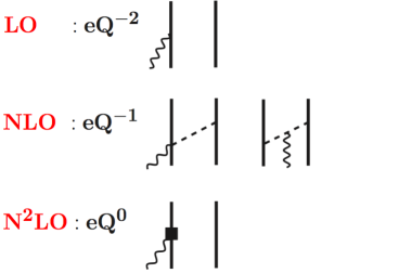
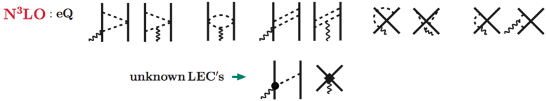
Figure 1: Contributions to the nuclear EM current ${\bf j}^{(n)}$. Nucleons, pions, and photons are represented by solid, dashed, and wavy lines, respectively.

and so on. These relations determine $\rho^{(n)}$, the leading order (LO) of which turns out to start at $n=-3$, and ${\bf j}^{(n)}$ with LO at $n=-2$. These contributions are illustrated diagrammatically for ${\bf j}^{(n)}$ in Fig. 1. The LO term involves the convection and spin magnetization currents of individual nucleons (their magnetic moments are taken from experiment), while the NLO one, which scales $Q^{-1}$, is due to one-pion exchange (OPE) and is well known—it is included in conventional calculations based on meson-exchange phenomenology. At N2LO a relativistic correction proportional to $1/m^{2}$—$m$ is the nucleon mass—to the LO single-nucleon current occurs, while two-pion exchange (TPE) loop corrections begin at N3LO or at order $Q$. At N3LO there are also tree-level contributions involving $\gamma\pi N$ vertices from sub-leading chiral Lagrangians, as well as contact terms from minimal and non-minimal couplings to the external EM field [10, 11].

There are 5 unknown LEC’s that enter ${\bf j}$, see Fig. 2, but none in $\rho$ [10, 11, 13, 14]. The operators derived so far have power law behavior for large momenta, and need to be regularized before they can sandwiched between nuclear wave functions. The regulator is taken of the form $C_{\Lambda}(k)={\rm exp}[-(k/\Lambda)^{n}]$ with $n=4$ and $\Lambda$ in the range 500-600 MeV. Then the two isoscalar LEC’s are fixed by reproducing the deuteron and isoscalar trinucleon magnetic moments, while two of the isovector LEC’s, $d_{1}^{V}$ and $d_{2}^{V}$ in Fig. 2, are constrained by assuming $\Delta$-resonance saturation [11]. Two different strategies have been adopted to fix the remaining isovector LEC: it is determined by reproducing either the $np$ radiative capture cross section $\sigma_{np}$ at thermal neutron energies or the isovector trinucleon magnetic moment $\mu^{V}$ [11]. There are no three-body currents entering at the order of interest [15], and so it is possible to use three-nucleon observables to fix some of these LEC’s.

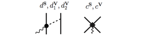
Figure 2: The isoscalar $d^{S}$ and $c^{S}$, and isovector $d_{1}^{V}$, $d_{2}^{V}$, and $c^{V}$ LEC’s characterizing the current at N3LO.

Their values are listed in Table 1. They are generally rather large, particularly when $c^{V}$ is fixed by the $np$ radiative capture cross section. The exception is the isoscalar LEC $d^{S}$ multiplying the one-pion exchange current involving a sub-leading $\gamma\pi N$ vertex from the chiral Lagrangian ${\cal L}^{(3)}_{\pi N}$.

$\Lambda$	$c^{S}$	$d^{S}\times 10$	$c^{V}(\sigma_{np})$	$c^{V}(\mu^{V})$
500	4.1	2.2	–13	–8.0
600	11	3.2	–22	–12

Table 1: Values for the LEC’s in units $1/\Lambda^{2}$ for $d^{S}$ and $1/\Lambda^{4}$ for $c^{S}$ and $c^{V}$; see text for further explanations.

3 Applications

Next, we discuss applications of nuclear $\chi$EFT to the few-nucleon systems, and defer to Saori Pastore’s talk [16] for results in the s- and p-shell nuclei. The few-nucleon results are obtained from chiral two-nucleon potentials developed by Entem and Machleidt at high order in the power counting ($Q^{4}$ or N3LO) [17, 18], and chiral three-nucleon potentials at leading order [19]. Following a suggestion by Gardestig and Phillips [20], the two LEC’s (in standard notation by now) $c_{D}$ and $c_{E}$ entering the latter have been constrained by fitting the Gamow-Teller matrix element in tritium $\beta$-decay and the binding energies of the trinucleons [21, 22].

3.1 Electromagnetic form factors of $A=2$–4 nuclei

The deuteron magnetic form factor is shown in Fig. 3 [11]. The bands reflect the sensitivity to cutoff variations in the range $\Lambda=500$–600 MeV. The black bands include all corrections up to N3LO in the (isoscalar) EM current. The NLO OPE and N3LO TPE currents are isovector and therefore give no contributions to this observable. The right panel of Fig. 3 contains a comparison of our results [11] with the results of a calculation based on a lower order potential and in which a different strategy was adopted for constraining the LEC’s $d^{S}$ and $c^{S}$ in the N3LO EM current [23]. This figure and the following Fig. 5 are from the recent review paper by S. Bacca and S. Pastore [24].

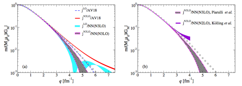
Figure 3: Magnetic form factor of the deuteron: the left panel shows results obtained with LO and N3LO currents and either the chiral N3LO or conventional AV18 potential; the right panel shows results obtained with N3LO currents and either the chiral N3LO (same as in left panel) or a chiral N2LO potential by Kölling et al.. The bands reflect cutoff variation. Experimental data are the empty circles.

The predicted magnetic form factors of the ³He and ³H ground states are compared to experimental data in Fig. 4 [11]. Isovector two-body terms in the EM current OPE and TPE play an important role in these observables, confirming previous results obtained in the conventional meson-exchange framework. We show the N3LO results corresponding to the two different ways used to constrain the LEC $c^{V}$ in the isovector contact current (recall the the LEC’s $d_{1}^{V}$ and $d_{2}^{V}$ are assumed to be saturated by the $\Delta$ resonance), namely by reproducing (i) the empirical value for the $np$ cross section—curve labeled N3LO($\sigma_{np}$)—or (ii) the isovector magnetic moment of ³He/³H—curve labeled N3LO($\mu^{V}$). The bands display the cutoff sensitivity ($\Lambda=500$–600 MeV), which becomes rather large for momentum transfers $q\gtrsim 3$ fm^-1. The N3LO($\sigma_{np}$) results are in better agreement with the data at higher momentum transfers; however, they overestimate $\mu^{V}$ by $\sim 2$%. On the other hand, the N3LO($\mu^{V}$) results, while reproducing $\mu^{V}$ by construction, underpredict $\sigma_{np}$ by $\sim 1$% .

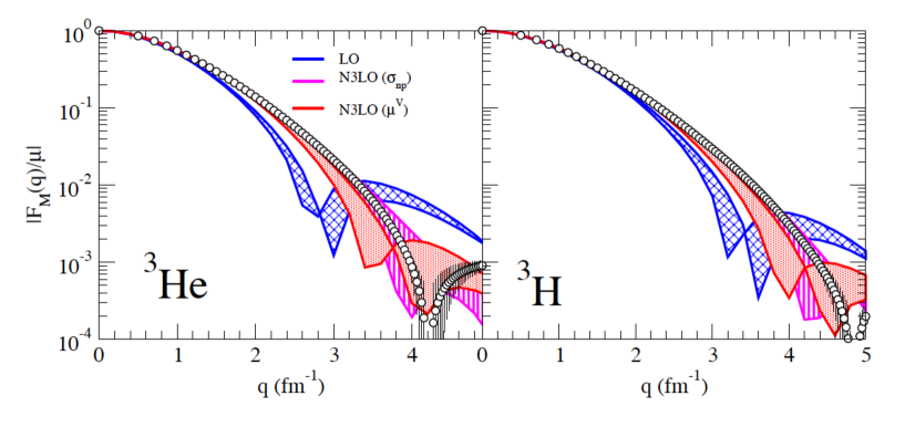
Figure 4: Magnetic form factors of ³He (left panel) and ³H (right panel); see text for further explanations.

Moving on to the EM charge operator, we show in Figs. 5 and 6 very recent calculations of the deuteron monopole and quadrupole form factors [11] and ⁴He (charge) form factor [25]. There are no unknown LEC’s beyond $g_{A}$, $f_{\pi}$ and the nucleon magnetic moments—the latter enter a relativistic correction, suppressed by $Q^{2}$ relative to the LO charge operator, i.e., the well-known spin-orbit term. The loop contributions (at N4LO) from two-pion exchange are isovector and hence vanish for these observables.

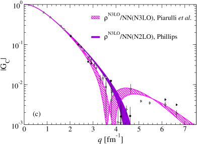
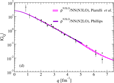
Figure 5: The deuteron monopole and quadrupole form factors obtained from measurements of the $A$ structure function and tensor polarization are compared to predictions based on N2LO and N3LO chiral potentials.

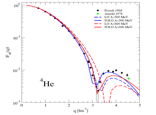
Figure 6: The ⁴He charge form factor obtained from elastic electron scattering data is compared to results obtained with the LO and N3LO charge operator.

The deuteron monopole and quadrupole form factor data are obtained from measurements of the $A$ structure function and tensor polarization observable in electron-deuteron scattering. In Fig. 5 the two bands correspond to two different calculations, one of which, labeled as NN(N2LO), is based on a lower order chiral potential [26, 27]. There is good agreement between theory and experiment. Differences between the two sets of theory predictions merely reflect differences in the deuteron wave functions obtained with the N3LO and N2LO potentials. These differences are amplified in the diffraction region of the monopole form factor.

The ⁴He charge form factor is obtained from elastic electron scattering cross section data. These data now extend up to momentum transfers $q\lesssim 10$ fm^-1 [28], well beyond the range of applicability of $\chi$EFT. In Fig. 6 only data up to $q\lesssim 5$ fm^-1 are shown. They are in excellent agreement with theory.

Predictions for the charge radii of the deuteron and helium isotopes and for the deuteron quadrupole moment ($Q_{d}$) are listed in Table 2 [11]. They are within 1% of experimental values. It is worth noting that until recently calculations based on the conventional meson-exchange framework used to consistently underestimate $Q_{d}$. However, this situation has now changed, and a relativistic calculation in the covariant spectator theory based on a one-boson exchange model of the nucleon-nucleon interaction has led to a value for the quadrupole moment [29] which is in agreement with experiment.

	$r_{c}$(2H)	$Q_{d}$	$r_{c}$(3He)	$r_{c}$(4He)
	(fm)	(fm2)	(fm)	(fm)
$\chi$EFT	2.126(4)	0.2836(16)	1.962(4)	1.663(11)
EXP	2.130(10)	0.2859(6)	1.973(14)	1.681(4)

Table 2: The charge radii of the ²H, ³He, and ⁴He nuclei, and ²H quadrupole moment.

3.2 Weak transitions in few-nucleon systems

Alessandro Baroni has discussed in this conference a recent derivation of the nuclear axial charge and current operators up to one loop (N4LO) in the TOPT formalism of Sec. 2 [30]. However, the results presented below have been obtained at N3LO in these weak transition operators (no loops). They are characterized by a single LEC in the axial current, which we fix by reproducing the Gamow-Teller (GT) matrix element in tritium $\beta$-decay [22].

A recent application of these transition operators is the calculation of the rates for $\mu^{-}$ capture on deuteron and ³He [22]. These rates have been predicted with $\sim 1$% accuracy,

$$\Gamma(^{2}{\rm H})=(399\pm 3)\,{\rm sec}^{-1}\ ,\qquad\Gamma(^{3}{\rm He})=(1494\pm 21)\,{\rm sec}^{-1}\ .$$

At this level of precision, it is necessary to also account for electroweak radiative corrections, which have been evaluated for these processes in Ref. [31]. The error quoted on the predictions above results from a combination of (i) the experimental error on the ³H GT matrix element used to fix the LEC in the axial current, (ii) uncertainties in the electroweak radiative corrections—overall, these corrections increase the rates by 3%–and (iii) the cutoff dependence.

There is a very accurate and precise measurement of the rate on ³He: $\Gamma^{\rm EXP}(^{3}{\rm He})=(1496\pm 4)$ sec^-1 [32]. We can use this measurement to constrain the induced pseudo-scalar form factor of the nucleon. We find $G_{PS}(q_{0}^{2}=-0.95\,m_{\mu}^{2})=8.2\pm 0.7$, which should be compared to a direct measurement on hydrogen at PSI, $G^{\rm EXP}_{PS}(q_{0}^{2}=-0.88\,m_{\mu}^{2})=8.06\pm 0.55$ [33], and a chiral perturbation theory prediction of $7.99\pm 0.20$ [34].

The situation for $\mu^{-}$ capture on ²H remains, to this day, somewhat confused: there is a number of measurements that have been carried out, but they all have rather large error bars. However, this unsatisfactory state of affairs should be cleared by an upcoming measurement by the MuSun collaboration at PSI with a projected 1% error.

Another recent example is the proton weak capture on protons [35, 36]. This process is important in solar physics: it is the largest source of energy and neutrinos in the Sun. The astrophysical $S$-factor for this weak fusion reaction is one of the inputs in the standard model of solar (and stellar) evolution [37]. A recent calculation based on N3LO chiral potentials including a full treatment of EM interactions up to order $\alpha^{2}$ ($\alpha$ is the fine structure constant), shows that it is now predicted with an accuracy of much less than 1%: $S(0)=(4.030\pm 0.006)\times 10^{-23}$ MeV-fm².

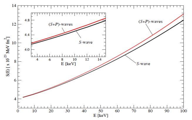
Figure 7: The $S$-factor for $pp$ weak fusion due to S- and (S+P)-wave capture as function of energy.

This calculation also included the (small) effects from capture of the two protons in relative P-wave, see Fig. 7 [36]. The increase due to P-wave capture offsets the decrease from higher order EM effects, in particular vacuum polarization.

3.3 Hadronic weak interactions in few-nucleon systems

Parity-violating (PV), but time-reversal invariant, chiral Lagrangians were constructed by Kaplan and Savage [38] in the early nineties up to order $Q$,

$${\cal L}_{\rm PV}=\overbrace{\frac{h^{1}_{\pi}}{2\sqrt{2}}\,f_{\pi}\,\overline{\psi}\,X^{3}_{-}\,\psi}^{{\cal L}_{\rm PV}^{(0)}}+{\cal L}^{(1)}_{\rm PV}\ ,$$

where $h^{1}_{\pi}$ is the PV $\pi NN$ coupling. More recently, their analysis has been extended to order $Q^{2}$, and a complete listing of isoscalar, isovector, and isotensor interactions up this order has been provided in Ref. [39]. These Lagrangians imply a PV potential that at order $Q$ depends on $h_{\pi}^{1}$ and 5 LEC’s (denoted as $C_{i}$ with $i=1,\dots,5$) multiplying short-range contact terms [39, 40, 41].

In principle one needs 6 independent measurements to constrain these LEC’s. A number of experiments has been performed: measurements of the longitudinal asymmetry in $\vec{p}$-$p$ scattering, of the photon asymmetry in the $np$ radiative capture, and of the neutron spin rotation in $\vec{n}$-$\alpha$ scattering. Some are in progress, such the measurement of the longitudinal asymmetry in the charge-exchange reaction ³He($\vec{n}$,$p$)³H, and some could be carried out, such as the measurement of the neutron spin rotation in $\vec{n}$-$d$ scattering. These are beautiful, but difficult experiments. For example, in a neutron spin rotation experiment one measures the rotation by an angle $\phi$ of the neutron spin in a plane perpendicular to the beam direction [42],

$$\frac{{\rm d}\phi}{{\rm d}d}=-\frac{2\pi\,\rho}{p}\,{\rm Re}\left[M_{+}(p;\theta=0)-M_{-}(p;\theta=0)\right]\ .$$

The effect depends on the density $\rho$ and length $d$ of the target, and on the difference between the helicity + and – forward scattering amplitudes ($p$ is the relative momentum). Its magnitude scales as $G_{F}\,f_{\pi}^{2}\sim 10^{-7}$.

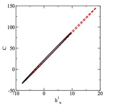
Figure 8: The left panel shows the data compared to results based on conventional strong-interaction potentials and the DDH meson-exchange model for the parity-violating potential. The right panel shows contour plots for the LEC’s $h_{\pi}^{1}$ and $C$, see text for further explanations.

In the following, we first discuss a recent attempt to constrain $h_{\pi}^{1}$ by considering the longitudinal asymmetry in $\vec{p}$-$p$ scattering [39]. There are 3 data points, two at low energy and one at relatively higher energy, see Fig. 8. Long-range contributions proportional to $h_{\pi}^{1}$ enter via two-pion exchange, and the asymmetry can be written as

$$A_{z}^{\,pp}(E,\Lambda)=a^{(pp)}_{0}(E,\Lambda)\,h^{1}_{\pi}+a^{(pp)}_{1}(E,\Lambda)\,C\ ,$$

with $C$ denoting the linear combination of contact LEC’s $C=C_{1}+C_{2}+2\,(C_{4}+C_{5})$. The 3 experimental data points do not uniquely determine $h_{\pi}^{1}$ and $C$: the right panel in Fig. 8 shows contour plots with a $\chi^{2}$-fit to these points. One finds two very narrow and partially overlapping ellipses corresponding to the cutoffs $\Lambda=500$ MeV and 600 MeV. There is a strong correlation between $h_{\pi}^{1}$ and $C$, and a rather large range of variability is allowed for these couplings. It tuns out that the two lowest data points are not independent, in the sense that their energy dependence is driven by that of the ¹S₀ strong-interaction phase [42].

$\Lambda$(MeV)	$a_{0}$	$a_{1}$	$a_{2}$	$a_{3}$	$a_{4}$	$a_{5}$
500	$-0.1444$	$0.0061$	$0.0226$	$-0.0199$	$-0.0174$	$-0.0005$
600	$-0.1293$	$0.0081$	$0.0320$	$-0.0161$	$-0.0156$	$-0.0001$

Table 3: Values for the coefficients $a_{i}$ entering the parameter $a_{z}$.

The next example is a recent analysis of the (longitudinal) asymmetry in the charge-exchange reaction ³He($\vec{n}$,$p$)³H [39]. It is given by $a_{z}\,\cos\theta$, where $\theta$ is scattering angle and the parameter $a_{z}$ can be expressed as

$$a_{z}=a_{0}\,h^{1}_{\pi}+a_{1}\,C_{1}+a_{2}\,C_{2}+a_{3}\,C_{3}+a_{4}\,C_{4}+a_{5}\,C_{5}\ .$$

The $a_{i}$ values are listed in Table 3: $a_{0}$ is about an order of magnitude larger than $a_{2}$, the largest among the coefficients multiplying the contact LEC’s. However, the (isoscalar) LEC $C_{2}$ is also expected to be large. Indeed, by matching the $C_{i}$ to the DDH estimates for the PV vector-meson couplings [43], one finds

$$C^{({\rm DDH})}_{1}\sim 1\ ,\quad C^{({\rm DDH})}_{2}\sim 30\ ,\quad C^{({\rm DDH})}_{3}\sim-2\ ,\quad C^{({\rm DDH})}_{4}\sim 0\ ,\quad C^{({\rm DDH})}_{5}\sim 7\ .$$

This indicates that the asymmetry $a_{z}\cos\theta$ results from the delicate balance between long-range OPE contributions and short-range contact contributions proportional to $C_{2}$.

4 Summary and outlook

We have provided an overview of $\chi$EFT results for the electroweak structure of few-nucleon systems. There is excellent quantitative agreement between experiment and theory, at least in the region of low energy and momentum transfer, where the $\chi$EFT approach is expected to be valid. In some instances, such as in muon capture, results with 1% accuracy are obtained. To echo the theme of one of the talks [44] in this conference, we are entering the precision era of nuclear $\chi$EFT.

Heavier nuclei offer new challenges and opportunities for applications of nuclear $\chi$EFT. The quantum Monte Carlo methods favored by our group to study nuclei with mass number $A>4$ are formulated in configuration space and, in particular, configuration-space potentials are needed. A first step in this direction is the very recent development of a class of minimally non-local two-nucleon chiral potentials that fit the $np$ and $pp$ scattering database up to lab energies of 300 MeV with $\chi^{2}$/datum close to 1.3 [45].

I wish to thank my collaborators A.Baroni, L.Girlanda, A.Kievsky, L.E.Marcucci, S.Pastore, M.Piarulli, and M.Viviani for their many contributions to the work presented in this talk. The support of the U.S.Department of Energy under contract DE-AC05-06OR23177 is also gratefully acknowledged.

References

- [1] J. Gasser and H. Leutwyler, Ann. Phys. (N.Y.) 158, 142 (1984).
- [2] N. Fettes, U.-G. Meissner, M. Mojzis, and S. Steininger, Ann. Phys. (N.Y.) 283, 273 (2000).
- [3] S. Weinberg, Phys. Lett. B 251, 288 (1990); Nucl. Phys. B 363, 3 (1991); Phys. Lett. B 295, 114 (1992).
- [4] C. Ordonez, L. Ray, and U. van Kolck, Phys. Rev. C 53, 2086 (1996).
- [5] E. Epelbaum, W. Gloeckle, and U.-G. Meissner, Nucl. Phys. A 637, 107 (1998).
- [6] T.-S. Park, D.-P. Min, and M. Rho, Phys. Rep. 233, 341 (1993).
- [7] T.-S. Park, D.-P. Min, and M. Rho, Nucl. Phys. A 596, 515 (1996).
- [8] S. Pastore, R. Schiavilla, and J.L. Goity, Phys. Rev. C 78, 064002 (2008).
- [9] S. Pastore, L. Girlanda, R. Schiavilla, and M. Viviani, Phys. Rev. C 84, 024001 (2011).
- [10] S. Pastore, L. Girlanda, R. Schiavilla, M. Viviani, and R.B. Wiringa, Phys. Rev. C 80, 034004 (2009).
- [11] M. Piarulli, L. Girlanda, L.E. Marcucci, S. Pastore, R. Schiavilla, and M. Viviani, Phys. Rev. C 87, 014006 (2013).
- [12] A. Baroni, L. Girlanda, S. Pastore, R. Schiavilla, and M. Viviani, arXiv:1509.07039.
- [13] S. Kölling, E. Epelbaum, H. Krebs, and U.-G. Meissner, Phys. Rev. C 80, 045502 (2009).
- [14] S. Kölling, E. Epelbaum, H. Krebs, and U.-G. Meissner, Phys. Rev. C 84, 054008 (2011).
- [15] L. Girlanda, A. Kievsky, L.E. Marcucci, S. Pastore, R. Schiavilla, and M. Viviani, Phys. Rev. Lett. 105, 232502 (2010).
- [16] S. Pastore, these proceedings.
- [17] D.R. Entem and R. Machleidt, Phys. Rev. C 68, 041001 (2003).
- [18] R. Machleidt and D.R. Entem, Phys. Rep. 503, 1 (2011).
- [19] E. Epelbaum, A. Nogga, W. Glöckle, H. Kamada, U.-G. Meissner, and H. Witala, Phys. Rev. C 66, 064001 (2002).
- [20] A. Gardestig and D.R. Phillips, Phys. Rev. Lett. 96, 232301 (2006).
- [21] D. Gazit, S. Quaglioni, and P. Navratil, Phys. Rev. Lett. 103, 102502 (2009).
- [22] L.E. Marcucci, A. Kievsky, S. Rosati, R. Schiavilla, and M. Viviani, Phys. Rev. Lett. 108, 052502 (2012).
- [23] S. Kölling, E. Epelbaum, and D.R. Phillips, arXiv:1209.0837.
- [24] S. Bacca and S. Pastore, J. Phys. G: Nucl. Part. Phys. 41, 123002 (2014).
- [25] L.E. Marcucci, F.L. Gross, M.T. Pena, M. Piarulli, R. Schiavilla, I. Sick, A. Stadler, J.W. Van Orden, and M. Viviani, J. Phys. G: Nucl. Part. Phys. in press, arXiv:1504.05063.
- [26] D.R. Phillips, Phys. Lett. B 567, 12 (2003).
- [27] D.R. Phillips, J. Phys. G 34, 365 (2007).
- [28] A. Camsonne et al., Phys. Rev. Lett. 112, 132503 (2014).
- [29] F.L. Gross, Phys. Rev. C 91, 014005 (2015).
- [30] A. Baroni, these proceedings.
- [31] A. Czarnecki, W.J. Marciano, and A. Sirlin, Phys. Rev. Lett. 99, 032003 (2007).
- [32] P. Ackerbauer et al., Phys. Lett. B 417, 224 (1998).
- [33] V.A. Andreev et al. (MuCap Collaboration), Phys. Rev. Lett. 110, 012504 (2013).
- [34] V. Bernard, N. Kaiser, and Ulf-G. Meissner, Phys. Rev. D 50, 6899 (1994); N. Kaiser, Phys. Rev. C 67, 027002 (2003).
- [35] T.-S. Park, L.E. Marcucci, R. Schiavilla, M. Viviani, A. Kievsky, S. Rosati, K. Kubodera, D.-P. Min, and M. Rho, Phys. Rev. C 67, 055206 (2003).
- [36] L.E. Marcucci, R. Schiavilla, and M. Viviani, Phys. Rev. Lett. 110, 192503 (2013).
- [37] J.N. Bahcall and M.H. Pinsonneault, Phys. Rev. Lett. 92, 121301 (2004).
- [38] D.B. Kaplan and M.J. Savage, Nucl. Phys. A 556, 653 (1993); Erratum ibid. A 570, 833 (1994); Erratum ibid. A 580, 679 (1994).
- [39] M. Viviani, A. Baroni, L. Girlanda, A. Kievsky, L.E. Marcucci, and R. Schiavilla, Phys. Rev. C 89, 064004 (2014).
- [40] L. Girlanda, Phys. Rev. C 77, 067001 (2008).
- [41] S.L. Zhu, C.M. Maekawa, B.R. Holstein, M.J. Ramsey-Musolf, and U. van Kolck, Nucl. Phys. A 748, 435 (2005).
- [42] R. Schiavilla, J. Carlson, and M. Paris, Phys. Rev. C 70, 044007 (2004).
- [43] B. Desplanques, J.F. Donoghue, and B.R. Holstein, Ann. Phys. (N.Y.) 124, 449 (1980).
- [44] E. Epelbaum, these proceedings.
- [45] M. Piarulli, L. Girlanda, R. Schiavilla, R. Navarro P rez, J.E. Amaro, and E. Ruiz Arriola, Phys. Rev. C 91, 024003 (2015).