Abstract

The stereoscopic imaging atmospheric Cherenkov technique, developed in the 1980s and 1990s, is now used by a number of existing and planned gamma-ray observatories around the world. It provides the most sensitive view of the very high energy gamma-ray sky (above $30\mathrm{\ GeV}$), coupled with relatively good angular and spectral resolution over a wide field-of-view. This Chapter summarizes the details of the technique, including descriptions of the telescope optical systems and cameras, as well as the most common approaches to data analysis and gamma-ray reconstruction.

Chapter 0 Atmospheric Cherenkov Gamma-ray Telescopes

1 Introduction

Astrophysical very high energy (VHE) gamma-rays (with energies $\gtrsim 30\mathrm{\ GeV}$) are believed to result almost exclusively from the interactions of populations of highly relativistic particles with ambient matter or photon fields. The study of these VHE photons therefore allows us to examine the processes of particle acceleration in the Universe, and the extreme environments in which they occur. Gamma-ray astronomy also provides a unique tool for many complementary astrophysical topics. For example, extragalactic background photon fields and intergalactic magnetic fields can be measured, or constrained, by their imprint on the measured properties of distant gamma-ray sources. Gamma-ray signatures of candidate dark matter particles may also lie in the VHE band, and can be sought through observations of regions in which the densest clumps of dark matter are believed to lie. Around 150 VHE gamma-ray sources have now been detected[1, 2] (Figure 1). These comprise many different source classes (pulsars and their nebulae, supernova remnants, and active galactic nuclei, to name a few) and the majority have been discovered using ground-based Atmospheric Cherenkov Telescopes (ACTs).

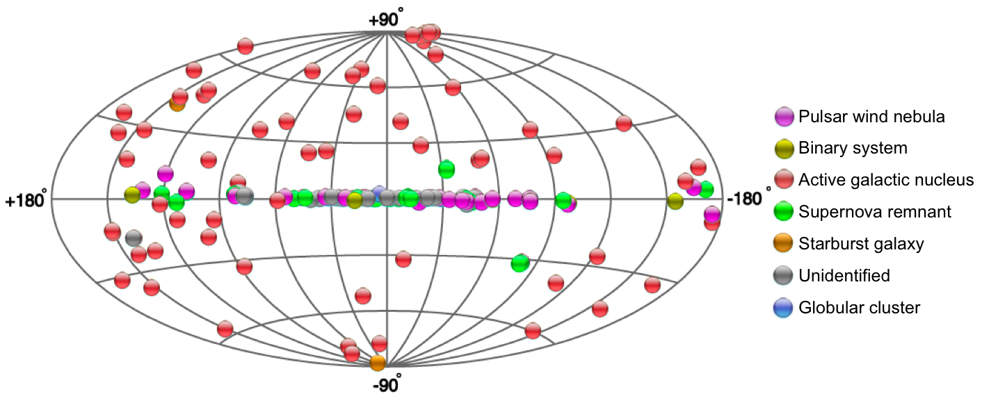
Figure 1: The locations, in Galactic coordinates, of all known astrophysical sources of TeV gamma-ray emission, as of 2015 (Figure courtesy of TeVCat.[1] See there for a full description of the different source classes).

The Earth’s atmosphere is opaque to high energy photons, and so the most direct approach to study the gamma-ray sky is to send detectors into space. However, astrophysical gamma-ray production mechanisms typically result in steeply falling power-law spectra, leading to a very low photon flux at high energies. The Crab Nebula, for example - one of the brightest astrophysical gamma-ray sources - produces a flux of only $\sim 6\mathrm{\ photons}\mathrm{\ m^{-2}}\mathrm{\ year^{-1}}$ at the Earth above $1\mathrm{\ TeV}$. To study the Universe at these energies therefore requires a detector with enormous collection area, far beyond the maximum practical size of a satellite-borne device (which is $\sim 1\mathrm{\ m^{2}}$). Atmospheric Cherenkov telescopes achieve this feat by measuring the Cherenkov light produced by gamma-ray triggered particle cascades (or air showers) in the atmosphere. In this way, using the Earth’s atmosphere as an intrisic part of the detection technique, effective collection areas can easily exceed $10^{5}\mathrm{\ m^{2}}$.

The potential of this approach for gamma-ray astronomy was first explored by Jelley and Galbraith in the 1950s[3], but attempts to exploit it were hampered by the overwhelming background of charged cosmic rays. The first significant discovery of an astrophysical TeV gamma-ray source was not made until the detection of the Crab Nebula, using the Whipple 10-meter telescope, in 1989[4]. This success was the result of the development of effective methods to record an image of the Cherenkov emission from air showers. A complete account of the long history and development of the field is given by Hillas.[5]

Three major ACT facilities are currently operating, the key properties of which are listed in Table 1. They each provide sensitivity to gamma-ray sources with a flux below $1\%$ of the steady flux from the Crab Nebula. Figure 2 shows one of these, the VERITAS array, with which the author is associated.

Details of each of the major atmospheric Cherenkov telescope facilities. Location Number Aperture Optical Number Field- of telescopes design of pixels of-view H.E.S.S. Namibia 4 $12\mathrm{\ m}$ Davies-Cotton 960 $5.0^{\circ}$ H.E.S.S. II${}^{\text{a}}$ Namibia 1 $28\mathrm{\ m}$ Parabolic 2048 $3.2^{\circ}$ MAGIC II La Palma 2 $17\mathrm{\ m}$ Parabolic 1039 $3.5^{\circ}$ VERITAS Arizona, USA 4 $12\mathrm{\ m}$ Davies-Cotton 499 $3.5^{\circ}$ ${}^{\text{a}}$H.E.S.S. II is an addition to the H.E.S.S. array, located in the centre of the four original telescopes.

Figure 2: The VERITAS atmospheric Cherenkov Telescope array.[6]

2 Air Showers and Atmospheric Cherenkov Emission

The design of atmospheric Cherenkov gamma-ray telescopes is driven by the essential characteristics of Cherenkov emission from air showers, which we first briefly describe.

A VHE gamma-ray incident on the Earth’s atmosphere converts into an electron-positron pair. Subsequent Bremsstrahlung and pair production interactions lead to the generation of an electromagnetic cascade in the atmosphere. The radiation length, $X_{0}$, for Bremsstrahlung in the atmosphere is $37.15\mathrm{\ g}\mathrm{\ cm^{-2}}$, which is 7/9 of the mean free path for pair production. This similarity allows a simple analytical approximation for the shower development (first developed by Heitler[7]), in which the total number of electrons, positrons and photons doubles every $\mathrm{ln}(2)X_{0}$. The primary gamma-ray energy, $E_{0}$, is split evenly among the secondary products. The shower continues to develop until the average electron energy drops to $E_{c}=84\mathrm{\ MeV}$, the critical energy below which ionization losses dominate. The maximum number of particles in the cascade is given by $E_{0}/E_{c}$.

Cosmic rays - charged, relativistic protons and nuclei - also produce air showers in the atmosphere. In this case, the cascade development is more complex, with hadronic interactions proceeding through a variety of channels, leading to the production of secondary nucleons, along with charged and neutral pions with large transverse momenta. The pions do not survive to sea level: neutral pions decay rapidly into two gamma-rays, while charged pions produce muons and neutrinos:

$$\pi^{o}\longrightarrow\gamma+\gamma$$

$$\pi^{+}\longrightarrow\mu^{+}+\nu_{\mu}$$

$$\pi^{-}\longrightarrow\mu^{-}+\bar{\nu}_{\mu}$$

The gamma-ray secondaries thus produced can trigger electromagnetic sub-showers, while the long-lived muons form the most penetrating component of the cascade, often reaching the ground. The result of this is that cosmic ray initiated air showers develop much less regularly than gamma-ray initiated cascades, as illustrated in Figure 3. These differences in the shower morphology, along with the reconstruction of the arrival direction of the incoming primary, allow ACTs to achieve an efficient discrimination of gamma-ray photons from the otherwise overwhelming isotropic cosmic ray background.

Figure 3: Monte Carlo simulations of the tracks of particles in photon and proton initiated air showers.[8] The first interaction height is fixed at $30\mathrm{\ km}$. The horizontal axis range is $\pm 5\mathrm{\ km}$.

The relativistic charged particles in air showers are moving faster than the speed of light in air ($v>c/n_{air}$, where $n_{air}$ is the refractive index) and so generate Cherenkov radiation. Cherenkov light is produced throughout the cascade development, with the maximum emission occurring when the number of particles in the cascade is largest, at an altitude of $\sim 10\mathrm{\ km}$ for primary gamma-ray energies of $100\mathrm{\ GeV}$ to $1\mathrm{\ TeV}$. Each particle generates Cherenkov light at a fixed angle to the direction of motion, ($\theta_{C}$), given by

$$\mathrm{cos}\theta_{C}=\frac{c}{vn_{air}}$$

The Cherenkov angle is $\sim 1.3^{\circ}$ at sea level. Electromagnetic cascade particles also undergo multiple Coulomb scattering, which distributes their directions over a small angular range and generates the shower’s lateral extent. The resultant filled “pool” of Cherenkov light on the ground has a photon density of $\sim 100\mathrm{\ photons}\mathrm{\ m^{-2}}$ for a $1\mathrm{\ TeV}$ gamma-ray primary, and a radial extent with a peak at $\sim 130\mathrm{\ m}$, as illustrated in Figure 4. The peak is due to a focussing effect resulting from the changing angle of Cherenkov emission with atmospheric depth.

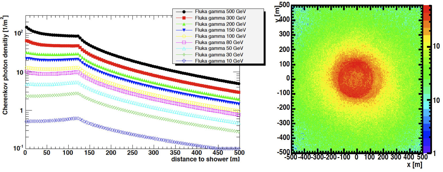
Figure 4: Monte Carlo simulations of the distribution of Cherenkov photons on the ground for gamma-ray initiated air showers. The left plot shows the Cherenkov photon density as a function of radial distance from the shower core for primaries with a range of energies, the right shows the two-dimensional photon density on the ground for a shower with a $300\mathrm{\ GeV}$ primary. Figure courtesy of G. Maier.

The Cherenkov photon yield is proportional to $1/\lambda^{2}$ (where $\lambda$ is the wavelength). The spectrum is therefore dominated by blue/UV emission, peaking around 340$\mathrm{\ nm}$. Shorter wavelength emission is subject to atmospheric absorption (particularly ozone), and therefore does not reach the ground, unless it is generated very deep in the atmosphere (for example by penetrating muons). Cherenkov photons from each shower arrive in a brief pulse of a few nanoseconds duration. The time-averaged photon yield from all air showers constitutes only $\sim 1/10000$th of the background night sky light in the visible, but the light from a single shower can rival the brightest objects in the night sky for the brief duration of the pulse.

3 Detection

The goal of an atmospheric Cherenkov gamma-ray telescope is to detect the Cherenkov emission from air showers, and to use this to determine the nature of the primary (gamma-ray or cosmic ray), along with its arrival direction and energy. The detection technique is, in essence, rather simple, requiring only a large mirror to collect Cherenkov photons, and a fast photon detector coupled to an oscilloscope to record them. The first detection of Cherenkov emission from an air shower was made with a $0.2\mathrm{\ m^{2}}$ reflector, a single photomultiplier tube (PMT) and a free-running analog oscilloscope.[9] Modern ACT arrays perform the same task, but can reach mirror areas $>600\mathrm{\ m^{2}}$, instrumented with thousands of PMTs coupled to GHz sampling electronics and sophisticated trigger systems.

While detection is relatively straightforward, gamma-ray discrimination and reconstruction is rather more challenging. One approach is to measure the arrival time and photon density distribution of the Cherenkov light at ground level. This “wavefront sampling” method was explored by experiments such as STACEE[10] and CELESTE[11], using the very large mirror areas provided by the heliostats of existing solar power facilities. The brightest previously known astrophysical gamma-ray sources were detected using this technique, but the difficulty of effective gamma-ray discrimination limited its usefulness. The technique may be more applicable at the highest energies($>10\mathrm{\ TeV}$), where small, widely separated detectors allow to achieve effective areas of $\sim 100\mathrm{\ km^{2}}$. This idea is currently being investigated by the HiSCORE experiment. [12]

By far the most successful approach, used by all of the major facilities in operation today, is the stereoscopic imaging technique. The principle of this is illustrated in Figure 5. Large convex reflectors are used to focus the Cherenkov light from air showers onto a camera comprised of photo-detector pixels. The camera records an image of the shower, and the properties of the image (its shape, intensity and orientation), allow determination of the properties of the shower primary. Applying this to an array of telescopes (“stereoscopy”) provides a view of the same shower from a number of different perspectives, and so enhances the geometrical shower reconstruction. It is worth stressing that a key aspect of this technique is the necessity for accurate Monte Carlo simulations of both the shower development and the detector response.

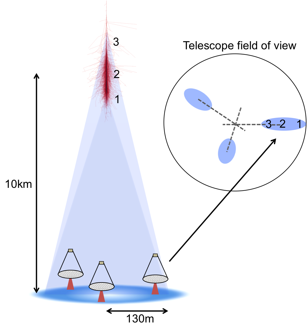
Figure 5: An illustration of the stereoscopic imaging technique. A gamma-ray triggers an electromagnetic cascade in the Earth’s atmosphere, which generates Cherenkov radiation in a pool on the ground. Telescopes within this light pool are used to form an image of the shower, which allows reconstruction of the arrival direction of the incident primary photon.

4 The Design of an Atmospheric Cherenkov Telescope Array

Since they observe blue Cherenkov light from air showers, atmospheric Cherenkov gamma-ray telescopes are effectively optical telescopes, working in the visible band of the electromagnetic spectrum. They are subject to the same constraints as other optical telescopes - observations must be conducted at night, under clear skies, at a dark site - but the design requirements are very different.

1 Optical systems

Two competing requirements inform the optical design of ACTs. The first is for a very large aperture, and hence mirror area. This allows one to collect as many Cherenkov photons as possible from each shower, which in turn defines the lowest gamma-ray energy threshold of the telescope. Fortunately, the relatively crude cameras of ACTs, and the lack of detailed structure in the Cherenkov images, means that the mirror form and surface quality is much less important than for optical telescopes. An optical point-spread-function of a few arcminutes is usually adequate. This level of performance can be achieved using tessellated reflectors, made up of hundreds of individual mirror facets.

The second requirement is for a large field-of-view. Cherenkov images from air showers are approximately elliptical in shape, with an angular extent of up to a few degrees. The images are offset from the arrival direction of the shower primary - in the case of gamma-ray initiated showers, this means that the image is offset from the gamma-ray source position in the field-of-view. The angular distance of the offset is proportional to the shower impact parameter (Figure 5). Even a point source of gamma-rays, therefore, requires a field-of-view of a few degrees diameter. In reality, many known sources of gamma-ray emission (particularly supernova remnants and pulsar wind nebulae) have a large angular extent. Additionally, analysis of ACT data typically uses a portion of the field-of view in which there are no known gamma-ray sources to estimate the background of remaining cosmic ray showers. Currently operating arrays have fields-of-view of $3^{\circ}-5^{\circ}$, while plans for the next generation of instruments reach $8^{\circ}-10^{\circ}$.

The requirement for a very large field-of-view for each telescope dictates a small focal ratio (focal length, $f$, divided by aperture, $D$) - typically around 1.0. Off-axis optical aberrations, particularly coma and astigmatism, are therefore an important consideration. A common approach for a tessellated reflector, used extensively for ACTs (starting with the Whipple 10-meter), was first developed by Davies and Cotton for a U.S. Army solar furnace facility - their original application was for the thermal testing of materials for military purposes.[13] In this design, individual spherical mirror facets, with a radius of curvature of twice the focal length of the telescope ($2f$), are placed on the surface of a spherical reflector with a radius equal to $f$. The facets are aligned such that the normals of the individual facets point to the $2f$ position along the optic axis. The reflector is therefore discontinuous at every point, and ideal performance is achieved with the smallest facets. As well as providing off-axis performance superior to that of a single spherical or parabolic reflector (Figure 6), the Davies-Cotton design uses identical mirror facets, which can be inexpensively mass-produced. Mirror facet alignment is also relatively simple. One downside, however, is that the design is not isochronous - the reflector induces some time spread in the arrival time of Cherenkov photons at the telescope cameras, typically on the order of a few nanoseconds. Tessellated parabolic reflectors, used by the world’s largest ACTs ( MAGIC and H.E.S.S. II), do not suffer from this drawback, but require facets of varying forms to be produced, with a corresponding increase in cost and complexity.

Figure 6: The image of a star viewed at different distances from the optic axis of a H.E.S.S. telescope, showing the effects of optical aberration in a Davies-Cotton optical system.[14]

Aplanatic two-mirror telescopes provide a solution to off-axis abberations, whilst retaining isochronicity and also reducing the plate scale in the focal plane significantly.[15] Cost and complexity again present challenges, but the benefits of two-mirror systems are such that they will very likely form a part of the next generation ACT arrays. Prototyping is already underway, with the Schwarzschild-Couder design among the favoured options.[16]

The technology for producing mirror facets is also a very active area of development.[17] Traditional techniques use milled aluminium, or glass which is “slumped” to the required shape, polished, and then coated with anodized aluminium. Carbon or glass fibre, aluminium honeycomb or a composite design can offer a more lightweight, cost-effective solution. With typically hundreds of mirror facets per telescope, alignment of the facets is not trivial. Stepper motors can be used to provide active mirror control, which greatly simplifies this task, as well as allowing for alignment corrections due to mechanical deformations during observations.

2 Telescope structure

The mechanical design of ACTs is also challenging, given the extremely large apertures, and the necessity of supporting a large, delicate and massive detector package at the prime focus. Weight and simplicity considerations have led to the adoption of altazimuth mounts for all modern ACTs. The rigidity requirements of the optical system and camera support structures have been solved in two ways - either by the brute force approach of constructing the telescope superstructure from a steel space frame (in the case of the H.E.S.S. and VERITAS telescopes, for example), or by the use of a lightweight carbon fibre frame coupled with an active mirror adjustment system (in the case of MAGIC, and planned for the largest next generation telescopes - see Figure 7).

The telescope is also required to track accurately - typically to within a few arcminutes. The position of the telescope is monitored by encoders (usually optical, with arcsecond resolution). A software model of the telescope pointing, calibrated using observations of stars, is used to translate these measurements into a position on the sky. The online tracking is supported by CCD pointing monitors, which are fixed to the telescope structure and track star positions, as well as the exact gamma-ray camera location. Offline corrections based on these CCD measurements are used to reduce systematic telescope pointing errors to typically tens of arcseconds.

ACTs must also be able to slew to new targets as rapidly as possible. The $40\mathrm{\ tonne}$, $17\mathrm{\ m}$ diameter MAGIC telescopes, for example, are able to move to observe any position in the sky within 40 seconds. This requirement is driven by the transient nature of the gamma-ray sky, which contains many sources known to flare dramatically on short timescales. In the case of gamma-ray bursts, the emission may last just a few seconds - although none of these have yet been detected from the ground, despite rapid slewing triggered by satellite alerts.

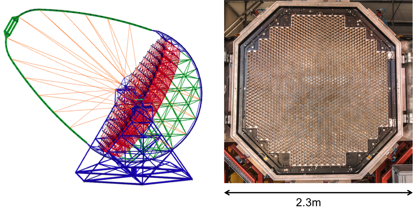
Figure 7: Left: The carbon fibre support structure design for the $23\mathrm{\ m}$ aperture Large Size Telescopes of the Cherenkov Telescope Array.[18]
Right: The PMT camera of the H.E.S.S. II telescope, containing 2048 PMTs and weighing 3 tonnes.[19]

3 Cameras

Large aperture, single-reflector ACTs require physically large cameras ($\geq 1\mathrm{\ m}$) to cover an adequately large field-of-view. In order to record an image, the photosensitive area must be divided into pixels, numbering hundreds or thousands, with each pixel sampling $\lesssim 0.1^{\circ}$. The photodetector pixel of choice for ACTs has, in most cases, been the photomultiplier tube (PMT). These devices provide reasonable photon detection efficiency ($\sim 20\%$), nanosecond response times, a large detection area, and extremely clean signal amplification (by factors of $\sim 100,000$), allowing them to easily resolve single photon signals. Dead space between the photo-sensitive areas of the individual pixels is recovered by placing close-packed light-concentrating Winston cones on the camera face. One example is the H.E.S.S. II PMT camera, shown in Figure 7, weighing 3 tonnes and containing 2048, $1.25\mathrm{\ inch}$ PMTs. The camera is housed at the telescope focal point, $36\mathrm{\ m}$ from the centre of the reflector dish, giving a field-of-view of $3.2^{\circ}$ in diameter (which is relatively small for an ACT).[19] While the size of ACTs prohibit the construction of domes around the complete telescopes, the expensive and delicate PMT cameras are usually housed in light-tight boxes, which allow for daytime testing and calibration. The H.E.S.S. II camera can actually be removed when required, and stored in a protective enclosure.

A number of recent technological advances are now finding their way into ACT camera design. PMT photocathode developments now yield quantum efficiencies of up to $40\%$ at short wavelengths (so-called “ultra-bialkali” devices). PMTs are now also available in “multianode” packages, in which an array of close-packed PMT cells are incorporated in a single housing, greatly reducing the cost per pixel of an ACT camera, and allowing for much finer pixellation of the field-of-view. Silicon photodetectors also show great promise, as demonstrated by the FACT (“First G-APD Cherenkov Telescope”) telescope, a small ($9.5\mathrm{\ m^{2}}$) pathfinder experiment, equipped with a camera containing 1440 individual Geiger-mode avalanche photodiode detectors.[20] Modern silicon-based devices can provide higher photon detection efficiency than PMTs, require lower operating voltages, and can cover large areas at relatively low cost - in particular with the development of Multi-Pixel Photon Counter (MPPC) arrays, containing arrays of up to 64 discrete detectors, each of which can be read out individually.

4 Trigger and Data Acquisition Systems

The arrival time of atmospheric Cherenkov flashes at the telescope is random and unpredictable. The flashes also last just a few nanoseconds, and exhibit temporal structure on timescales even shorter than this. Continuously monitoring the sky with GHz sampling rates on hundreds or thousands of channels is impractical; instead, it is necessary to trigger the data acquisition system of ACTs, such that the photo-detector outputs are recorded only for a small time window around the arrival time of the Cherenkov flash. Since the trigger decision time is longer than the duration of the flash itself, the photodetector output signals must be delayed (e.g. by routing analog signals through long cables), or continuously sampled and stored in digital memory buffers. Upon receipt of a valid trigger, the relevant data time window can be accessed and saved to disk as digital samples.

Trigger systems typically work on multiple levels - the design goal being to trigger on the faintest possible Cherenkov flashes, without incurring a prohibitively high rate of false triggers due to the fluctuating night sky background. Individual pixels are equipped with discriminators, which produce a digital output. The outputs for each camera are passed to a logic circuit which looks for spatial coincidences (e.g. 3 neighbouring pixels must have triggered within a few nanoseconds). The final trigger decision occurs at the array level - typically at least 2 telescope cameras must have triggered at the same time, after correction for the different path lengths of the Cherenkov light to each telescope. Many variations on this basic scheme exist, notably the analog sum-trigger developed for use on the MAGIC telescopes.[21] Figure 8 shows a“bias curve” for the VERITAS array, illustrating the changing event rate as a function of individual pixel discriminator threshold, for each of the four telescopes, and for the complete array.

Figure 8: Left: A“bias curve” for the VERITAS array. The rate of triggers is shown as a function of the discriminator threshold chosen for all of the PMT pixels. The upper curves correspond to the individual telescope rates, the lower curve to the complete array, after requiring a coincident trigger from at least two telescopes. A clear break point is seen at the transition between triggers dominated by night sky background fluctuations, and those dominated by cosmic ray air showers. The dashed line indicates a typical threshold setting for standard operations.
Right: Data products for a VERITAS telescope, consisting of a digitized signal trace for each PMT in the 499 pixel camera. The image in the camera has been cleaned, by setting the signal to zero in all pixels which contain no Cherenkov light. The ellipse shows a simple moment-based parameterization of the image.

Prior to digitization, the photo-detector outputs are pre-amplified, as close to the sensor as possible. This boosts the signal strength without significantly increasing the signal-to-noise ratio, and allows PMT detectors (in particular) to run at lower gain - extending their useful lifetime, and protecting them from damage due to bright DC light sources, including stars in the field-of-view. Since the Cherenkov flashes sit upon a continuous DC background of night sky light, the signals are also AC-coupled at this point. Digitization is accomplished in various different ways - historically, simple integrating Analog-to-Digital Converters (ADCs) were used, while more modern systems use flash-ADCs or custom-designed analog ring sampling devices, operating at multi-GHz sampling speeds. The final data products consist of a sampled (or integrated) signal trace for every pixel for each triggered event (Fig. 8). The data rate of modern ACTs is in excess of a few hundred recorded events per second, and reaches a few KHz for the largest telescopes.

5 Peripheral and Environmental Systems

In addition to the telescopes themselves, a wide variety of peripheral systems are usually deployed, associated with calibration and monitoring tasks, both of the telescopes and of the atmosphere above them. Telescope calibration requires nanosecond light pulsers, used to flat-field the photodetector gains, and to measure their single photon response. Atmospheric monitoring can be achieved with local weather stations, and with LIDARs, optical telescopes, and infra-red radiometers, which can reveal the presence of clouds by measuring the radiative temperature of the night sky.

6 Array Design

To this point, we have focussed on the design of individual telescopes; however, the use of multiple telescopes in concert dramatically increases the sensitivity of the technique, along with its angular and spectral resolution. Numerous studies have been performed on the optimum layout and spacing of ACT arrays.[22, 23, 24] The conclusions can broadly be summarized as follows: (i) more telescopes are better, with the array sensitivity increasing roughly as the square root of the number of telescopes, and (ii) the optimal spacing depends upon the energy range to be covered: wider spacing provides best sensitivity for higher energies. One further point to note is that the array performance changes when the array becomes significantly larger than the Cherenkov light pool.[25] In this regime the central region of the Cherenkov light pool is always sampled by multiple telescopes (unlike smaller arrays, where the shower core often lies outside of the area enclosed by the array). The result of this is appreciably better sensitivity at low energies, for telescopes of relatively modest size.

5 ACT Data Analysis

The analysis of ACT data is complex, and the details have comparable impact on the sensitivity and performance of the array as do many aspects of the hardware. To recap, the goal of the the analysis is to identify the primary particle, and to reconstruct its arrival direction and energy. This information is then used to assess the statistical significance of any gamma-ray signal, to map its distribution on the sky, and to reconstruct the gamma-ray flux and energy spectrum. Many different analysis methods exist in the literature, and the details vary between the different arrays. Here we describe the most common techniques in broad detail, and conclude with a brief summary of some of the more sophisticated methods in use.

1 Flat-fielding and Image Cleaning

The raw data products for ACTs consist of a digitally sampled signal trace for each of the photosensors in the cameras, roughly centered on the arrival time of the Cherenkov pulse (Fig. 8). The first stage of the data processing consists of measuring and subtracting the signal pedestal value - the baseline value in the absence of any Cherenkov photons. The next step is to identify those pixels which contain a Cherenkov signal, above some pre-defined threshold. The signals are then corrected for variations in the photodetector gain values, measured using a calibration light pulse. The result of this pre-processing is a cleaned, calibrated image, typically approximately elliptical in shape (Fig. 8).

2 Identification of the Primary

Even for a moderately strong gamma-ray source, cosmic ray shower images outnumber gamma-ray shower images by at least a factor of $\sim 10^{5}$. Effective separation of the gamma-ray events is therefore crucial. In the case of a point source of gamma rays, by far the most effective tool for discrimation is the arrival direction of the primary - but many TeV sources have large angular extent, up to a few degrees in diameter. Fortunately, significant differences in the Cherenkov image morphology, originating in the differences in the air shower development, make discrimination possible - despite the relatively crude optics and camera pixellation of an ACT.[26]

The cleaned images are parameterized by a simple moment analysis, in which their $width$, $length$ and orientation are calculated. Gamma-ray images are typically less wide, and shorter, than cosmic ray images with similar Cherenkov intensity and impact parameter. In the case of a single telescope, simply selecting images with small $width$ and $length$ provides fair discrimination.[27] The power of this analysis is dramatically increased, however, when multiple telescopes view the same shower. In this case, the shower core location, and hence the impact distance from each telescope ($R$), can be determined to within an accuracy of $\sim 10\mathrm{\ m}$. The core location is reconstructed geometrically; in the reference frame of the array, all images point away from the shower core location, and so the core can be found by intersecting the image major axes.

Once the core location is known, the measured $width$ of the image can be compared with a prediction, $width_{MC}$, for images with the same Cherenkov intensity, $s$. This prediction, with an associated spread, $\sigma_{width}$, is derived from detailed Monte Carlo simulations of the air shower development and the telescope response. The predicted widths are typically stored in look-up tables, a number of which are generated corresponding to various different conditions under which the observations were taken (e.g. elevation angle, background night-sky brightness). The result of this comparison is then combined for all of the Cherenkov images of the shower ($N_{images}$) like so:

$$mscw=\frac{1}{N_{images}}\left[\sum_{i=1}^{N_{images}}\frac{width_{i}-width_{MC}(R,s)}{\sigma_{width}(R,s)}\right]$$

$mscw$ is known as the“mean-scaled width”, and is used to provide effective discrimation between gamma-ray and cosmic ray initiated events[28, 29] (Figure 9). A similar method can be applied to the image $length$. Various other parameters have also been derived and used with different degrees of success (e.g. height of shower maximum, Cherenkov photon arrival time gradient along the shower).

For the purposes of gamma-ray astronomy, a simple discrimination between gamma rays and all other primaries is usually all that is required. ACTs can also serve as powerful tools for cosmic ray physics, however, and attempts have been made to measure the spectrum and composition of the nuclear cosmic ray flux[30, 31], as well as the electron component.[32]

3 Arrival Direction Reconstruction

Reconstruction of the arrival direction of the shower primary serves two purposes: it provides effective discrimination between gamma-ray photons from the source and the isotropic charged cosmic ray background, and it allows us to study and to map out the gamma-ray emission. Accurate location of the point of origin of the gamma-ray emission is often necessary to the identification of gamma-ray sources, and gamma-ray mapping of extended astrophysical sources provides clues to the particle acceleration processes at work in these objects.

In the field-of-view of the telescopes, the major axes of the image ellipses intersect at the point corresponding to the arrival direction of the primary particle, as shown schematically in Figure 5. This fact is used to provide an estimate of the arrival direction, usually with some weighting scheme which gives additional weight to the axes of the brightest images.[33] The resulting angular resolution of the technique is energy dependent, with typically $68\%$ of the gamma rays from a point source reconstructed to within $0.1^{\circ}$ of the source location, for energies around $1\mathrm{\ TeV}$. At lower energies, fluctuations in the shower development, and low Cherenkov photon statistics, degrade the resolution somewhat.

Once the arrival directions have been calculated, any point in the field-of-view can be tested for evidence for gamma-ray emission, by selecting those events which lie within a pre-defined radius around the test point. This process is complicated by the fact that the gamma-ray emission from each point lies on top of the remaining background of misidentified cosmic ray events. In order to calculate the gamma-ray excess, and to calculate the statistical significance of this excess, it is therefore necessary to find an independent estimate of the remaining background at each point. This is accomplished by measuring the background rate in blank regions of the sky, from which little or no gamma-ray emission is expected. These “OFF-source” regions can be selected in a variety of different ways: for example by dedicated observations of adjacent fields-of-view, or (more commonly) by selecting regions within the same field-of-view, but offset from the test position. In this latter case, particular care must be taken to account for the varying detection efficiency across the field-of-view. A full description of a sample of common background estimation techniques is given by Berge et al[34].

Once the background is known, the gamma-ray excess at any position can be measured, and its significance calculated[35] (or an upper limit to the number of excess events, in the case of no detection). By testing a range of positions on a 2-D grid, a map of gamma-ray emission on the sky can be constructed. Figure 9 shows an example of a gamma-ray excess map from the direction of a supernova remnant, as measured by the H.E.S.S. telescope array. Converting the excess (or upper limit) into a measurement of the photon flux from the source (in$\mathrm{\ photons}\mathrm{\ cm^{-2}}\mathrm{\ s^{-1}}$), requires detailed modelling of the energy-dependent effective area of the telescope array, as described in the following section.

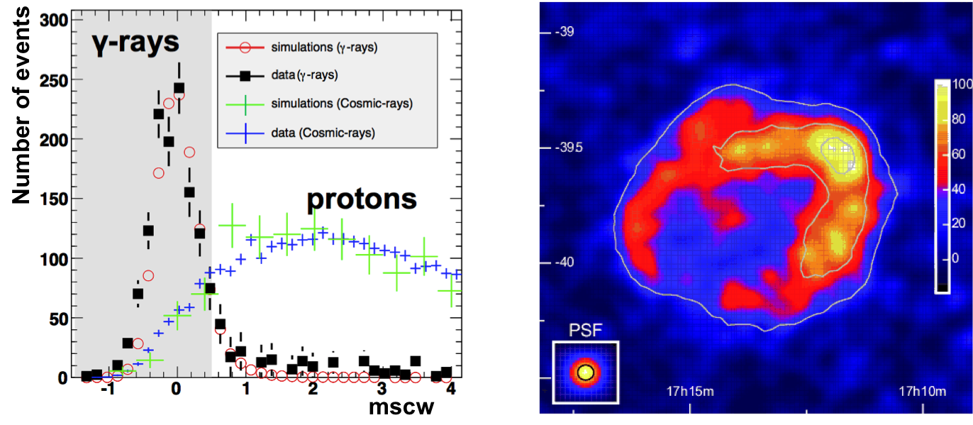
Figure 9: Left: The distribution of the mean-scaled width for gamma-rays and cosmic rays, from Monte Carlo simulations and for a real gamma-ray source. Selecting events within the shaded region provides effective discrimination of gamma-ray events from the hadronic background
Right: H.E.S.S. map of gamma-ray emission from the supernova remnant RX J1713.7-3946.[36]

4 Gamma-Ray Energy, Flux and Spectrum

Calculation of the energy of an incident gamma-ray relies upon the fact that, to a good approximation, the number of particles in the shower, and hence the Cherenkov photon yield, is directly proportional to the primary energy. Measuring the Cherenkov emission intensity, and combining this with the distance to the shower, therefore allows an estimate of the gamma-ray energy.[37] Multiple telescopes improve this energy estimate dramatically, since they provide multiple measurements of the shower light yield, and an improved estimate of the shower core location.[38]

In practice, the energy estimate is made by referring to look-up tables which contain the predicted gamma-ray energy as a function of impact parameter and Cherenkov intensity. The contents of the tables are derived from Monte Carlo simulations of the shower development, and of the telescope response. For the purposes of energy estimation, the most important parameter of the telescope model is the single photo-electron response of the photo-detectors and their read-out electronics. The most important factor in simulating the Cherenkov yield at the telescope mirrors is the Earth’s atmosphere. This is much more difficult to monitor and account for, and hence introduces systematic uncertainties at the level of at least $10\%$. Numerous tables are generated, corresponding to different observing conditions (elevation angle, background night-sky brightness, source offset in the field-of-view). The energy resolution of the technique depends upon the energy of the primary, reaching typically $\sim 15\%$ above $1\mathrm{\ TeV}$, and degrading below this.

Converting the measured energy distribution of gamma-rays from a source into a meaningful flux estimate, or energy spectrum, requires knowledge of the effective area of the detector. In the case of ACTs, the maximum effective area is determined by the size of the Cherenkov light pool, rather than by the size of the telescopes or the area of the array, and can reach $>10^{5}\mathrm{\ m^{2}}$ at high energies. At lower energies, the trigger efficiency of the array (and hence the effective area) drops sharply, eventually reaching zero. The energy-dependent effective area is calculated by simulating gamma-ray showers over a wide range of impact parameters, and with an energy distribution similar to a typical source (e.g. a power law with an index of $-2.0$). The ratio of the number of triggered events to the number of events simulated, multiplied by the area over which the events were thrown, then gives the effective area. The effective area again depends upon a wide variety of operating conditions (elevation, sky brightness) and analysis parameters (gamma-ray selection cuts, exact analysis method), which must be precisely matched between the data analysis and the simulations.

The reconstructed energy distribution of gamma-ray events from a source can then be divided by the energy-dependent effective area in order to reconstruct the true energy spectrum of the source. Systematic biases can arise due to the fact that the effective area estimate depends upon the simulated gamma-ray spectrum (due to the finite energy resolution of the instrument). This can be addressed by recalculating the effective area using the fitted energy spectrum iteratively, until the two converge. More sophisticated unfolding methods are also used to account for the finite resolution of the technique.[39]

Gamma-ray source spectra are smooth continua, typically well-fit by straight or curved power laws, or by a power-law with an exponential cutoff. The spectra can be most easily parameterized by fitting a chosen form to the gamma-ray flux points using the least-squares method. A more sophisticated approach, less prone to biases introduced by binning the data, is to perform a maximum-likelihood estimation of the spectral parameters, taking into account the effective area and the energy-resolution function of the detector.[40]

5 Alternative Analysis Methods

The analysis methods described above were developed by the Whipple and HEGRA collaborations in the 1990s. They are robust against changing conditions, provide good sensitivity, and are widely used to this day. However, the development of analysis tools has always proceeded in parallel with the hardware developments of ACTs, and many alternative methods exist in the literature. Some of these provide significance improvements in sensitivity, energy threshold, or angular or spectral resolution.

One flaw of the standard method is that it does not take advantage of the fact that an array provides multiple views of the same shower, and so the images recorded should be correlated. This additional information can be exploited by performing a global fit to the data, using a model of the shower development based on the primary energy, arrival direction and impact parameter. The first implementation of this method was made by the CAT collaboration, using just a single telescope, and a simple analytical 2-D model of the shower profile.[41] The technique has subsequently been refined to work with multiple telescopes, to perform a log-likelihood minimisation using all pixels in the camera[42], and to use 3D analytical models of the shower development[43], or direct comparison with template images generated by Monte Carlo simulations.[44] In these schemes, the goodness-of-fit parameter provides a single powerful discriminant to separate gamma-rays from background. The method also automatically provides an energy estimate, which can be used to reconstruct spectra.

Another approach is to improve the discrimination between gamma-ray and cosmic ray events through the use of advanced pattern recognition or multivariate analysis techniques. Some of the most successful approaches to this draw on developments in the field of experimental particle physics, where similar problems of classification are often met. While many different techniques have been attempted (neural networks, genetic algorithms, etc.), the most efficient appear to be the decision tree methods: boosted decision trees[45, 46, 47] and random forests.[48] Inputs to these machine learning algorithms can correspond to the simple geometrical parameters of the standard analysis method, or encompass additional information, including the results of the template fitting methods described above.

Finally, many attempts have been made to explore additional properties of the Cherenkov radiation from air showers, in the hope of finding complementary information to enhance the analysis. Some have failed - the spectrum[49] or the polarization[50] of the Cherenkov light, for example, do not seem likely to provide any useful additional discrimination. The arrival time of Cherenkov photons, however, does improve discrimination somewhat - an aspect of the analysis that becomes more important with the development of very large isochronous reflectors, and very fast ($\geq 1\mathrm{\ GHz}$) sampling electronics.[51, 52, 53]

6 Concluding Remarks

Atmospheric Cherenkov gamma-ray telescopes have proven remarkably successful over the past decade. Small arrays of moderately-sized telescopes have opened a new window on the Universe, probing particle acceleration in extreme environments both within and outside of our Galaxy. The next stage in the development of the technique requires substantial investment, and hence collaboration on a global scale. This is proceeding through the “Cherenkov Telescope Array” (CTA) project, which is designing and constructing a next generation instrument.[54] The plan involves a km² array with a few large aperture ($\sim 23\mathrm{\ m}$) telescopes at the centre, surrounded by an array of moderately-sized telescopes ($\sim 10\mathrm{\ m}$) with $\sim 100\mathrm{\ m}$ spacing, supplemented by a wider-spaced array of smaller telescopes ($4\mathrm{\ m}$). A graded array such as this is expected to provide sensitivity improvements of an order of magnitude over current arrays, together with the widest possible energy coverage. Prototyping and testing is underway, and new technologies are being tested at all stages (e.g. in mirror designs, photosensors, and trigger and data acquisition systems). The goal of such development is not only to enhance the array performance, but also to deal with the necessities of mass production, low cost, and strict maintenance requirements. Both northern and southern hemisphere arrays are envisaged, and possible sites are currently under discussion.

References

- 1. S. P. Wakely and D. Horan. http://tevcat.uchicago.edu/.
- 2. J. Holder, Astroparticle Physics. 39, 61–75, (2012).
- 3. J. V. Jelley and W. Galbraith, Journal of Atmospheric and Terrestrial Physics. 6, 304–312, (1955).
- 4. T. C. Weekes et al., ApJ. 342, 379–395, (1989).
- 5. A. M. Hillas, Astroparticle Physics. 43, 19–43, (2013).
- 6. The VERITAS Collaboration. /http://veritas.sao.arizona.edu/.
- 7. W. Heitler, Quantum theory of radiation. 1954.
- 8. F. Schmidt. Images produced using the CORSIKA package. http://www.ast.leeds.ac.uk/~fs/showerimages.html.
- 9. W. Galbraith and J. V. Jelley, Nature. 171, 349–350, (1953).
- 10. D. M. Gingrich et al., IEEE Transactions on Nuclear Science. 52, 2977–2985, (2005).
- 11. E. Paré et al., Nuclear Instruments and Methods in Physics Research A. 490, 71–89, (2002).
- 12. M. Tluczykont et al., Astroparticle Physics. 56, 42–53, (2014).
- 13. J. M. Davies and E. S. Cotton, Solar Energy. 1, 16–22, (1957).
- 14. R. Cornils et al., Astroparticle Physics. 20, 129–143, (2003).
- 15. V. Vassiliev, S. Fegan, and P. Brousseau, Astroparticle Physics. 28, 10–27, (2007).
- 16. V. V. Vassiliev and S. J. Fegan, International Cosmic Ray Conference. 3, 1445–1448, (2008).
- 17. G. Pareschi et al. vol. 8861, Society of Photo-Optical Instrumentation Engineers (SPIE) Conference Series, (2013).
- 18. G. Ambrosi et al., ArXiv e-prints. 1307.4565, (2013).
- 19. J. Bolmont et al., Nuclear Instruments and Methods in Physics Research A. 761, 46–57, (2014).
- 20. H. Anderhub et al., Nuclear Instruments and Methods in Physics Research A. 639, 58–61, (2011).
- 21. J. R. García et al., ArXiv e-prints. (2014).
- 22. W. Hofmann et al., Astroparticle Physics. 13, 253–258, (2000).
- 23. P. Colin and S. LeBohec, Astroparticle Physics. 32, 221–230, (2009).
- 24. K. Bernlöhr et al., Astroparticle Physics. 43, 171–188, (2013).
- 25. S. J. Fegan and V. V. Vassiliev, International Cosmic Ray Conference. 3, 1441–1444, (2008).
- 26. A. M. Hillas, International Cosmic Ray Conference. 3, 445–448, (1985).
- 27. M. Punch et al., International Cosmic Ray Conference. 1, 464, (1991).
- 28. A. Daum et al., Astroparticle Physics. 8, 1–11, (1997).
- 29. HEGRA Collaboration, Astroparticle Physics. 10, 275–289, (1999).
- 30. F. Aharonian et al., Phys. Rev. D. 59(9), 092003, (1999).
- 31. F. Aharonian et al., Phys. Rev. D. 75(4), 042004, (2007).
- 32. F. Aharonian et al., A&A. 508, 561–564, (2009).
- 33. W. Hofmann et al., Astroparticle Physics. 12, 135–143, (1999).
- 34. D. Berge, S. Funk, and J. Hinton, A&A. 466, 1219–1229, (2007).
- 35. T.-P. Li and Y.-Q. Ma, ApJ. 272, 317–324, (1983).
- 36. F. Aharonian et al., A&A. 464, 235–243, (2007).
- 37. G. Mohanty et al., Astroparticle Physics. 9, 15–43, (1998).
- 38. F. Aharonian et al., ApJ. 614, 897–913, (2004).
- 39. J. Albert et al., Nuclear Instruments and Methods in Physics Research A. 583, 494–506, (2007).
- 40. A. Djannati-Atai et al., A&A. 350, 17–24, (1999).
- 41. S. Le Bohec et al., Nuclear Instruments and Methods in Physics Research A. 416, 425–437, (1998).
- 42. M. de Naurois and L. Rolland, Astroparticle Physics. 32, 231–252, (2009).
- 43. M. Lemoine-Goumard, B. Degrange, and M. Tluczykont, Astroparticle Physics. 25, 195–211, (2006).
- 44. R. D. Parsons and J. A. Hinton, Astroparticle Physics. 56, 26–34, (2014).
- 45. S. Ohm, C. van Eldik, and K. Egberts, Astroparticle Physics. 31, 383–391, (2009).
- 46. A. Fiasson et al., Astroparticle Physics. 34, 25–32, (2010).
- 47. Y. Becherini et al., Astroparticle Physics. 34, 858–870, (2011).
- 48. J. Albert et al., Nuclear Instruments and Methods in Physics Research A. 588, 424–432, (2008).
- 49. A. M. Hillas, Space Science Reviews. 75, 17–30, (1996).
- 50. I. de la Calle et al., Astroparticle Physics. 17, 133–149, (2002).
- 51. M. Heß et al., Astroparticle Physics. 11, 363–377, (1999).
- 52. E. Aliu et al., Astroparticle Physics. 30, 293–305, (2009).
- 53. V. Stamatescu et al., Astroparticle Physics. 34, 886–896, (2011).
- 54. B. S. Acharya et al., Astroparticle Physics. 43, 3–18, (2013).