The dust content of damped Lyman-$\mn@boldsymbol{\alpha}$ systems in the Sloan Digital Sky Survey

Abstract

The dust-content of damped Lyman-$\alpha$ systems (DLAs) is an important observable for understanding their origin and the neutral gas reservoirs of galaxies. While the average colour-excess of DLAs, $E(B\!-\!V)$, is known to be $\la$15 milli-magnitudes (mmag), both detections and non-detections with $\sim$2 mmag precision have been reported. Here we find 3.2-$\sigma$ statistical evidence for DLA dust-reddening of 774 Sloan Digital Sky Survey (SDSS) quasars by comparing their fitted spectral slopes to those of $\sim$7000 control quasars. The corresponding $E(B\!-\!V)$ is $3.0\pm 1.0$ mmag, assuming a Small Magellanic Cloud (SMC) dust extinction law, and it correlates strongly (3.5-$\sigma$) with the metal content, characterised by the Si ii $\lambda$1526 absorption-line equivalent width, providing additional confidence that the detection is due to dust in the DLAs. Evolution of $E(B\!-\!V)$ over the redshift range $2.1<z<4.0$ is limited to $<$2.5 mmag per unit redshift (1-$\sigma$), consistent with the known, mild DLA metallicity evolution. There is also no apparent relationship with neutral hydrogen column density, $N_{\textsc{h\scriptsize{\,i}}}$, though the data are consistent with a mean $E(B\!-\!V)/N_{\textsc{h\scriptsize{\,i}}}=(3.5\pm 1.0)\times 10^{-24}$ mag cm², approximately the ratio expected from the SMC scaled to the lower metallicities typical of DLAs. We implement the SDSS selection algorithm in a portable code to assess the potential for systematic, redshift-dependent biases stemming from its magnitude and colour-selection criteria. The effect on the mean $E(B\!-\!V)$ is negligible ($<$5 per cent) over the entire redshift range of interest. Given the broad potential usefulness of this implementation, we make it publicly available.

1 Introduction

Currently, the only direct way to probe the neutral gas surrounding early galaxies is to study its absorption against background objects. Damped $\textrm{Ly-}\alpha$ systems (DLAs) – defined as having a neutral hydrogen column densities of $N_{\textsc{h\scriptsize{\,i}}}=2\times 10^{20}$ cm^-2 in absorption (Wolfe et al., 1986) – provide rich information about this gas, particularly when observed along the sight-lines to quasars, i.e. relatively bright, very compact objects. At such column densities, the gas in DLAs is self-shielded against the ultraviolet background radiation from galaxies and quasars, so it is predominantly neutral (e.g. Viegas, 1995), enabling very precise metallic element abundances to be measured. However, some metals (e.g. C, Mg, Fe, Cr) will be preferentially incorporated into dust grains (Jenkins, 1987; Pettini et al., 1997), so a complete and accurate understanding of the nucleosynthetic history of DLA gas requires some knowledge of its dust content. This is also an important factor in identifying possible $\alpha$-element enhancements in DLAs (e.g. Vladilo, 2002; Ledoux et al., 2002). Further, dust grains are the formation sites for most molecular hydrogen in cool DLA gas (Jenkins & Peimbert, 1997; Ledoux et al., 2003) and provide surfaces for photoelectric heating of DLAs (Wolfe et al., 2003a, b). Understanding the dust content of DLAs is therefore important for determining their astrophysical origins and significance.

DLAs are cosmologically important because they contain most of the neutral gas at all redshifts up to at least $z=5$ (e.g. Wolfe, 1986; Lanzetta et al., 1995; Prochaska et al., 2005; Prochaska & Wolfe, 2009; Noterdaeme et al., 2009b; Crighton et al., 2015). However, if dust in DLAs obscures a significant proportion of the background quasars from flux-limited and/or colour-selected quasar surveys (Ostriker & Heisler, 1984), the comoving mass density of DLA gas, $\Omega_{\textrm{\scriptsize g}}^{\textrm{\scriptsize DLA}}$, will be underestimated (e.g. Fall & Pei, 1993). This may be a particularly acute concern if, as one may naively expect, higher-$N_{\textsc{h\scriptsize{\,i}}}$ DLAs contain more dust, because DLAs with $N_{\textsc{h\scriptsize{\,i}}}\sim 10^{21}$ cm^-2 have the largest contribution to $\Omega_{\textrm{\scriptsize g}}^{\textrm{\scriptsize DLA}}$ despite their relative paucity (e.g. see figures 10 and 14 of Prochaska et al. 2005 and Noterdaeme et al. 2009b, respectively). Surveys of DLAs in radio-selected quasar samples avoid dust bias, though obtaining large enough samples is much more difficult. For example, the combined samples of Ellison et al. (2005) and Jorgenson et al. (2006) contain 26 DLAs identified towards 119 quasars and yield a $\Omega_{\textrm{\scriptsize g}}^{\textrm{\scriptsize DLA}}$ which is a factor of $\sim$1.3 higher than optically-selected surveys, but with a 33 per cent uncertainty. Therefore, attempts to determine $\Omega_{\textrm{\scriptsize g}}^{\textrm{\scriptsize DLA}}$ with $\la$20 per cent accuracy must incorporate other, possibly tighter constraints on DLA dust content.

The most direct indicators of dust in DLAs would be the carbonaceous 2175 Å ‘dust bump’ absorption feature and the silicate dust features at 10 and 18 $\mu$m (e.g. Draine, 2003). The dust bump is ubiquitous in Milky Way studies but less prominent in sight-lines through the Large Magellanic Cloud (LMC) and seemingly absent in the Small Magellanic Cloud (SMC). Given the broad undulations and small variations in quasar continua, clear dust bump detections are difficult and rare. Indeed, just three detections in bona fide DLAs have been reported (Junkkarinen et al., 2004; Noterdaeme et al., 2009a; Ma et al., 2015), though several have been reported in strong Mg ii absorbers (e.g. Wang et al., 2004; Zhou et al., 2010; Jiang et al., 2010; Wang et al., 2012). The silicate features are also rare: the 10 $\mu$m feature has been detected in two bona fide DLAs (Kulkarni et al., 2007; Kulkarni et al., 2011) and 5 other strong quasar absorbers (Kulkarni et al., 2011; Aller et al., 2012, 2014). Using these features to determine the average DLA dust content appears unlikely, if not impossible, though they clearly allow the chemical and physical characteristics of the dust in some DLAs to be studied.

The average DLA dust content may be better determined by measuring the reddening it should impart to the spectra of the background quasars. The significant variation in quasar colours means that this is an inherently statistical approach, with large samples of quasars with foreground DLAs (‘DLA quasars’) and, importantly, larger samples without DLAs (‘non-DLA quasars’) to act as ‘controls’, required to detect small amounts of dust. Early attempts (Fall & Pei, 1989; Fall et al., 1989) culminated in a $>$4-$\sigma$ detection of average DLA reddening of $\Delta\beta=0.38\pm 0.13$ (Pei et al., 1991) with 26 DLA quasars and 40 non-DLA quasars, where $\beta$ represents the spectral index when the quasar continuum flux density is fitted as

$$f_{\lambda}\propto\lambda^{\beta}\,.$$ (1)

This implied that 10–70 per cent of bright quasars at redshift $z=3$ were being missed in optical surveys (Fall & Pei, 1993). The Sloan Digital Sky Survey (SDSS) increased the available DLA and non-DLA quasar samples significantly and ensured a more uniform quasar selection. Using 70 DLA quasars and $\sim$1400 non-DLA quasars, Murphy & Liske (2004) found no evidence for DLA dust reddening at $2.1<z<3.9$, with $\Delta\beta$ constrained to be $<$0.19 at 3-$\sigma$ confidence, inconsistent with previous results. Assuming an SMC dust reddening law, the rest-frame colour excess of DLA dust reddening was limited to $E(B\!-\!V)_{\textrm{\scriptsize SMC}}<20$ milli-magnitudes (mmag) at 3-$\sigma$ confidence. This stringent limit indicates a very low average DLA dust content and illustrates the large, careful analysis required to detect dust via this statistical approach.

More recent SDSS-based analyses have provided a mix of apparent detections and other limits on DLA dust reddening at similar redshifts ($2.2\la z\la 3.5$). Using the photometric colours of 248 DLA quasars from the SDSS Data Release (DR) 5, Vladilo et al. (2008) found a $\approx$3.5-$\sigma$ indication of reddening with rest-frame $E(B\!-\!V)_{\textrm{\scriptsize SMC}}\approx 6$ mmag. Frank & Péroux (2010) compared composite spectra, made from stacking DR7 spectra in the rest-frame of 676 DLAs, with composites from non-DLA quasars ‘matched’ in redshift and magnitude. This indicated no DLA reddening, $E(B\!-\!V)_{\textrm{\scriptsize SMC}}=-1.7\pm 2.2$ mmag, $\approx$2.9 $\sigma$ lower than Vladilo et al. (2008)’s result. Khare et al. (2012) performed a similar analysis using 1084 $\log(N_{\textsc{h\scriptsize{\,i}}}/\textrm{cm}^{-2})\geq 20.0$ absorbers [i.e. including ‘sub-DLAs’, or ‘super Lyman-limit systems’, with $20.0\leq\log(N_{\textsc{h\scriptsize{\,i}}}/\textrm{cm}^{-2})<20.3$], finding no evidence for reddening from the absorbers, consistent with Frank & Péroux. Most recently, Fukugita & Ménard (2015) used the photometric colours of 1211 sub-DLA and DLA quasars from DR9 in the restricted absorption redshift range $2.1<z_{\textrm{\scriptsize abs}}<2.3$, finding a relatively large $E(B\!-\!V)_{\textrm{\scriptsize SMC}}\approx 10$ mmag with $\sim$4-$\sigma$ significance. These recent results are discussed further in Section 6.

Given the variety of recent results, it is important to further consider the average dust content of DLAs. Here we use DR7 spectra to measure the spectral index, $\beta$ in Equation (1), and hence $E(B\!-\!V)$ for an assumed dust extinction law, in 774 SDSS DLA quasars. We also constrain how the dust content depends on redshift, gas column density and metal-line strength with the aim of finding clues to the origin and physical/chemical nature of the dust and the DLAs themselves. However, as with previous SDSS-based studies, we must recall that the SDSS quasars targetted for spectroscopy were selected based on their colours. In principle, this could lead to a bias towards or against dusty DLAs (i.e. redder spectra) in the SDSS quasar sample. Given the complicated, redshift-dependent nature of the colour-selection algorithm (Richards et al., 2002), this bias should also be redshift-dependent. Here we consider in detail the effect of colour selection bias on the measured colour excess from DLA dust for the first time. We demonstrate the effect to be negligible at all redshifts we consider ($2.1<z_{\textrm{\scriptsize abs}}<4.0$).

This paper is organised as follows. Section 2 describes the quasar and DLA samples used in this work and how control samples were established for all DLA quasars. Section 3 explains how the spectral index and colour excess were measured for each DLA. Section 4 details the main results while discussion and comparison with other recent results is deferred to Section 6. We test the effects of colour-selection bias in Section 5 and Appendix A describes our emulation of the SDSS quasar colour selection algorithm of Richards et al. (2002) and basic tests to ensure its reliability for this work. Given the broad potential usefulness of this code, we have provided it in Bernet & Murphy (2015). Our main conclusions are summarized in Section 7.

2 Quasar and DLA sample definitions

2.1 Quasar catalogues, spectra and exclusions

The results presented in this paper are derived from the SDSS DR7 versions of the spectra identified as quasars in the catalogue of Schneider et al. (2010). This catalogue contains 105783 quasars with improved (where necessary) emission redshift measurements compared with those automatically determined by the original SDSS data processing system. We exclude the 6214 broad absorption line (BAL) quasars identified in this catalogue by Shen et al. (2011) because the BAL features may have interfered with the DLA identification procedure (see Section 2.2) and because BAL quasars are often heavily reddened compared to the normal distribution of quasar colours (e.g. Reichard et al., 2003). We also exclude quasars with emission redshifts outside the range $2.20\leq z_{\textrm{\scriptsize em}}\leq 4.42$. The lower redshift cut ensures a non-zero search path for DLAs redwards of the blue limit of the SDSS spectra (i.e. $\approx$3800 Å) while the higher redshift cut ensures that the reddest band we use to determine the quasar spectral index (quasar rest-frame wavelengths 1684–1700 Å; see Section 3) remains entirely bluewards of the red limit of the SDSS spectra (i.e. $\sim$9200 Å). These redshift restrictions leave 14672 quasars (note the further restrictions on the quasar sample below in Section 2.2).

We also cross-checked our main results using both the DR5 and DR7 spectra of the quasars identified in the DR5 quasar catalogue of Schneider et al. (2007), and find consistent results. A new reduction and spectrophotometric calibration was introduced in DR6, yielding a 30 mmag root-mean-square (RMS) difference between the $r-i$ colours from the point-spread-function (PSF) photometry and those synthesized from the calibrated spectra of stars. The spectrophotometry of DR9 spectra is expected to be biased because smaller fibres were used (2 vs. 3″ diameter, respectively) and, without atmospheric dispersion compensation available, they were offset to collect blue light at the expense of red light to probe the $\textrm{Ly-}\alpha$ forest (Pâris et al., 2012).

2.2 DLA samples

The baseline results in this paper were derived using DLAs from the catalogue of Noterdaeme et al. (2009b). They searched DR7 spectra of objects that the automatic SDSS data processing labelled as quasars with $z_{\textrm{\scriptsize em}}>2.17$. The search was restricted to 8339 spectra with median continuum-to-noise ratios (CNRs) exceeding 4 per pixel (pix^-1) redwards of the wavelength where the signal-to-noise ratio (SNR) first exceeds 4 pix^-1. Noterdaeme et al. (2009b) applied an automated algorithm to detect DLAs and determine their $z_{\textrm{\scriptsize abs}}$, $N_{\textsc{h\scriptsize{\,i}}}$ and rest equivalent widths of selected metal lines, e.g. $W_{\textrm{\scriptsize r}}(\textrm{C\,{{ii}}}\,\lambda{1334})$ and more often $W_{\textrm{\scriptsize r}}(\textrm{Si\,{{ii}}}\,\lambda{1526})$.

From the 14672 DR7 quasars selected in Section 2.1 we removed the 6743 quasars that were not among those searched for ‘strong absorbers’ by Noterdaeme et al. (2009b), leaving 7929 quasars. These ‘strong absorbers’ include DLAs and sub-DLAs systems with $\log(N_{\textsc{h\scriptsize{\,i}}}/\textrm{cm}^{-2})\geq 20.0$ cm^-2. Our main results and much of our discussion below focus on the DLAs only. However, as a cross-check on possible systematic effects and to boost sample sizes when searching for trends within our results, we also perform the same analyses with the sub-DLAs included.

The final restriction on the quasar and absorber samples is to remove quasar spectra in which Noterdaeme et al. (2009b) identified more than one ‘strong absorber’. This last selection criterion defines our baseline samples as follows:

• DLA & non-DLA samples: 7879 quasars; 774 are DLA quasars (i.e. with a single, bona fide DLA); 7105 are non-DLA quasars.

• Absorber & non-absorber samples: 7802 quasars; 1069 are absorber quasars [i.e. with a single $\log(N_{\textsc{h\scriptsize{\,i}}}/\textrm{cm}^{-2})\geq 20.0$ cm^-2 system]; 6733 are non-absorber quasars.

Note that this last criterion means that the DLA$+$non-DLA sample is larger than the absorber$+$non-absorber sample. This is because sub-DLAs are more common than DLAs, and because sub-DLAs are allowed in the DLA and non-DLA quasar spectra but only a single DLA or sub-DLA is allowed in the absorber quasars. That DLA quasars are allowed to be ‘contaminated’ by sub-DLAs is offset by the contamination of non-DLA quasars in the same way and in approximately equal proportion, thereby leaving a negligible residual effect on the differential reddening measurement we make in Section 3.

Tables 1–4 provide the relevant information for each of these samples, including the basic (sub-)DLA parameters used in the reddening analysis below. Figure 1 shows the redshift distributions of the DLA quasars and the DLAs themselves. Note the relative paucity of DLA quasars with $z_{\textrm{\scriptsize em}}<2.9$: quasar colours cross the stellar locus between $z_{\textrm{\scriptsize em}}\sim 2.5$–3.0, so the SDSS colour-selection algorithm had to be specially modified there even to select some quasars. This is one example of the strongly varying, complicated quasar colour selection function in the SDSS. By comparison, Figure 1 shows that the DLA redshift distribution is relatively smooth.

Table 1: The DLA quasar sample (774 quasars). The quasars are listed by their SDSS name (formed from right ascension and declination), emission redshift ($z_{\textrm{\scriptsize em}}$), the redshift search path for DLAs defined by $z_{\rm min}$ and $z_{\rm max}$ [see Equation (3)], the measured spectral index, $\beta$, and its 1-$\sigma$ uncertainty ($\sigma_{\beta}$), and the spectral index measured with an unweighted power-law fit, $\beta_{\rm nw}$. The DLA properties required in our analysis are the absorption redshift ($z_{\textrm{\scriptsize abs}}$), logarithmic column density, $\mathcal{N}_{\textsc{h\scriptsize{\,i}}}\equiv\log(N_{\textsc{h\scriptsize{\,i}}}/\textrm{cm}^{-2})$, the rest-frame equivalent widths $W_{\textrm{\scriptsize r}}(\textrm{Si\,{{ii}}}\,\lambda{1526})$ and $W_{\textrm{\scriptsize r}}(\textrm{C\,{{ii}}}\,\lambda{1334})$ (with non-detections indicated by “$-999.00$”), the measured difference, $\Delta\beta$, between the DLA quasar’s $\beta$ and the mean $\beta$ of its control distribution, the corresponding colour excess, $E(B\!-\!V)$, for SMC and LMC-like dust, and the number of control quasars ($N_{\rm ctrl}$). The full table is available in the electronic version of this paper (see the Supporting Information).

SDSS name	$z_{\textrm{\scriptsize em}}$	$z_{\rm min}$	$z_{\rm max}$	$\beta$	$\sigma_{\beta}$	$\beta_{\rm nw}$	$z_{\textrm{\scriptsize abs}}$	$\mathcal{N}_{\textsc{h\scriptsize{\,i}}}$	$W_{\rm r}$ [Å]		$\Delta\beta$	$E(B\!-\!V)$ [mag]		$N_{\rm ctrl}$
(J2000)									Si ii $\lambda$1526	C ii $\lambda$1334		SMC	LMC
001240.57$+$135236.7	$3.1866$	$2.371$	$3.116$	$-1.266$	$0.104$	$-1.273$	$3.022$	$20.86$	$-999.00$	$-999.00$	$0.195$	$0.0130$	$0.0184$	497
001328.20$+$135828.0	$3.5755$	$2.501$	$3.499$	$-1.371$	$0.060$	$-1.389$	$3.281$	$21.56$	$0.30$	$0.34$	$0.073$	$0.0051$	$0.0078$	160
001813.89$+$142455.6	$4.2355$	$3.409$	$4.147$	$-1.672$	$0.170$	$-1.184$	$3.861$	$20.65$	$-999.00$	$-999.00$	$-0.162$	$-0.0110$	$-0.0166$	29
003501.88$-$091817.6	$2.4187$	$2.224$	$2.361$	$-1.608$	$0.080$	$-1.601$	$2.337$	$20.42$	$-999.00$	$-999.00$	$-0.063$	$-0.0041$	$-0.0059$	545
005319.20$+$134708.8	$2.9203$	$2.275$	$2.855$	$-1.332$	$0.077$	$-1.332$	$2.628$	$20.92$	$-999.00$	$0.62$	$0.146$	$0.0107$	$0.0175$	352

Table 2: The absorber quasar sample (1069 quasars). The columns are defined in the caption of Table 1 and the full table is available in the electronic version of this paper (see the Supporting Information).

SDSS name	$z_{\textrm{\scriptsize em}}$	$z_{\rm min}$	$z_{\rm max}$	$\beta$	$\sigma_{\beta}$	$\beta_{\rm nw}$	$z_{\textrm{\scriptsize abs}}$	$\mathcal{N}_{\textsc{h\scriptsize{\,i}}}$	$W_{\rm r}$ [Å]		$\Delta\beta$	$E(B\!-\!V)$ [mag]		$N_{\rm ctrl}$
(J2000)									Si ii $\lambda$1526	C ii $\lambda$1334		SMC	LMC
001240.57$+$135236.7	$3.1866$	$2.371$	$3.116$	$-1.266$	$0.104$	$-1.273$	$3.022$	$20.86$	$-999.00$	$-999.00$	$0.196$	$0.0125$	$0.0176$	457
001328.20$+$135828.0	$3.5755$	$2.501$	$3.499$	$-1.371$	$0.060$	$-1.389$	$3.281$	$21.56$	$0.30$	$0.34$	$0.091$	$0.0062$	$0.0092$	140
001813.89$+$142455.6	$4.2355$	$3.409$	$4.147$	$-1.672$	$0.170$	$-1.184$	$3.861$	$20.65$	$-999.00$	$-999.00$	$-0.214$	$-0.0162$	$-0.0261$	26
003126.79$+$150739.5	$4.2832$	$3.432$	$4.195$	$-2.904$	$0.156$	$-2.427$	$4.083$	$20.28$	$-999.00$	$-999.00$	$-1.512$	$-0.0984$	$-0.1367$	31
003501.88$-$091817.6	$2.4187$	$2.224$	$2.361$	$-1.608$	$0.080$	$-1.601$	$2.337$	$20.42$	$-999.00$	$-999.00$	$-0.063$	$-0.0043$	$-0.0062$	538

Table 3: The non-DLA quasar sample (7105 quasars). The columns are defined in the caption of Table 1 and the full table is available in the electronic version of this paper (see the Supporting Information).

SDSS name (J2000)	$z_{\textrm{\scriptsize em}}$	$z_{\rm min}$	$z_{\rm max}$	$\beta$	$\sigma_{\beta}$	$\beta_{\rm nw}$
000050.60$-$102155.9	$2.6404$	$2.136$	$2.579$	$-2.056$	$0.045$	$-2.018$
000143.41$+$152021.4	$2.6383$	$2.152$	$2.578$	$-1.150$	$0.069$	$-1.158$
000221.11$+$002149.3	$3.0699$	$2.136$	$3.001$	$-1.422$	$0.053$	$-1.428$
000300.34$+$160027.6	$3.6983$	$3.545$	$3.619$	$-1.496$	$0.145$	$-1.088$
000413.64$-$085529.6	$2.4241$	$2.153$	$2.366$	$-1.300$	$0.037$	$-1.323$

Table 4: The non-absorber quasar sample (6733 quasars). The columns are defined in the caption of Table 1 and the full table is available in the electronic version of this paper (see the Supporting Information).

SDSS name (J2000)	$z_{\textrm{\scriptsize em}}$	$z_{\rm min}$	$z_{\rm max}$	$\beta$	$\sigma_{\beta}$	$\beta_{\rm nw}$
000050.60$-$102155.9	$2.6404$	$2.136$	$2.579$	$-2.056$	$0.045$	$-2.018$
000143.41$+$152021.4	$2.6383$	$2.152$	$2.578$	$-1.150$	$0.069$	$-1.158$
000221.11$+$002149.3	$3.0699$	$2.136$	$3.001$	$-1.422$	$0.053$	$-1.428$
000300.34$+$160027.6	$3.6983$	$3.545$	$3.619$	$-1.496$	$0.145$	$-1.088$
000413.64$-$085529.6	$2.4241$	$2.153$	$2.366$	$-1.300$	$0.037$	$-1.323$

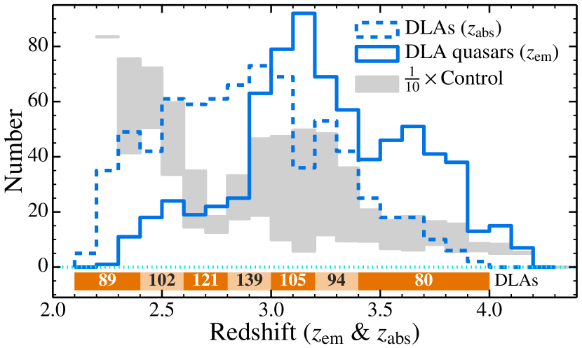
Figure 1: Emission redshift ($z_{\textrm{\scriptsize em}}$) distributions of DLA quasars (solid line) and their corresponding control quasars (shaded regions), and the absorption redshift ($z_{\textrm{\scriptsize abs}}$) distribution of the DLAs themselves. There is a single DLA per DLA quasar. For each $\Delta z=0.1$ bin, the shaded region indicates the range in sizes of the control samples for the DLA quasars in that bin. Note that these shaded regions are normalized by a factor of 10 for clarity; for example, the minimum and maximum number of control quasars corresponding to any of the DLA quasars with $3.0\leq z_{\textrm{\scriptsize em}}<3.1$ is 99 and 473, respectively. The shaded bar below the histograms, labelled with the number of DLAs in each bin, shows the absorption redshift bins used in subsequent figures.

While the SDSS spectral resolving power ($R\approx 1800$) and the CNR and SNR thresholds ensure that most DLAs are identified, they are not optimal for accurately estimating $N_{\textsc{h\scriptsize{\,i}}}$. To cross-check our main results against different approaches to estimating $N_{\textsc{h\scriptsize{\,i}}}$ we used the alternative, albeit smaller sample of DLAs from DR5 by Prochaska & Wolfe (2009); it provides results consistent with those presented here. Although their DLA search employed similar SNR threshold criteria to Noterdaeme et al. (2009b), their approach to fitting the DLAs to estimate $N_{\textsc{h\scriptsize{\,i}}}$ differs, so we expect that a comparison of results from the two samples is a reasonable test for biases, particularly at low $N_{\textsc{h\scriptsize{\,i}}}$. Using the ‘statistical sample’ from Prochaska & Wolfe (2009), and a similar series of exclusions as we applied above to the Noterdaeme et al. (2009b) sample, left 526 DLA quasars and 7712 non-DLA quasars.

2.3 Control samples

From the non-DLA samples above (Section 2.2), a sample of “control” quasars is selected for each DLA quasar to benchmark the typical distribution of quasar spectral indices expected in the absence of strong absorbers. To be selected as a control quasar for a given DLA quasar with redshift $z_{\textrm{\scriptsize em}}^{\rm DLA}$ and DLA redshift $z_{\textrm{\scriptsize abs}}^{\rm DLA}$, a non-DLA quasar with redshift $z_{\textrm{\scriptsize em}}$ must satisfy the following criteria:

$$z_{\textrm{\scriptsize em}}^{\rm DLA}-0.05\leq z_{\textrm{\scriptsize em}}\leq z_{\textrm{\scriptsize em}}^{\rm DLA}+0.05;~{}~{}{\rm and}$$ (2)

$$z_{\rm min}\leq z_{\textrm{\scriptsize abs}}^{\rm DLA}\leq z_{\rm max}\,.$$ (3)

Here, $z_{\rm min}$ and $z_{\rm max}$ define, respectively, the minimum and maximum redshifts between which the non-DLA quasar spectrum was searched for DLAs by Noterdaeme et al. (2009b). These values were kindly provided to us by P. Noterdaeme. The maximum redshift, $z_{\rm max}$, was defined for all quasars to be 5000 $\textrm{km\,s}^{-1}$ bluewards of $z_{\textrm{\scriptsize em}}$ so as to avoid strong absorbers associated with the quasars themselves. This means that both the DLA and non-DLA samples defined above may have such “associated” DLAs and sub-DLAs in their spectra. However, again, this will occur with very similar frequency in both the DLA and non-DLA samples, so the differential reddening measurement will not be significantly affected. Similar criteria are applied when forming the control samples for absorber quasars from the non-absorber sample. The minimum redshift, $z_{\rm min}$, was defined by Noterdaeme et al. according to the CNR and SNR criteria mentioned in Section 2.2. This means that $z_{\rm min}$ effectively acts as a spectral quality control measure to ensure that DLAs can be securely identified between $z_{\rm min}$ and $z_{\rm max}$.

The first criterion above reflects the requirement for control quasars to have similar redshifts as their corresponding DLA quasar. It defines a small redshift interval within which we assume the complicated, redshift-dependent SDSS quasar selection biases are relatively constant. It effectively determines the number of control quasars for a given DLA quasar; increasing it increases the control sample size but risks larger effects from non-uniformities in the quasar selection. Reducing it substantially below $\pm$0.05 decreases the control samples of many DLA quasars. We find that our results are insensitive to changes in this interval up to $\pm$0.2.

The second criterion above states that a non-DLA quasar can only qualify as a control quasar for a given DLA quasar (with a DLA at $z_{\textrm{\scriptsize abs}}$) if a hypothetical DLA at $z_{\textrm{\scriptsize abs}}$ could have been found within in its spectrum. For that to be true, $z_{\textrm{\scriptsize abs}}$ must lie between the $z_{\rm min}$ and $z_{\rm max}$ values of the non-DLA quasar. Inherent in this criterion is the assumption that DLA dust extinction and reddening are small: if they were large, and such a dusty DLA was placed between $z_{\rm min}$ and $z_{\rm max}$ in a non-DLA spectrum, it would suppress the continuum flux in the $\textrm{Ly-}\alpha$ forest region, and $z_{\rm min}$ would increase, potentially to the point where the second criterion is no longer satisfied. In this sense, the CNR and SNR thresholds in the DLA search algorithm, combined with the second criterion above, may slightly diminish the measured DLA dust reddening signal compared to its true strength. However, the bias will reduce in proportion to the reddening itself, and will likely be negligible at the very small reddening levels observed in our work. Simple tests, in which $z_{\rm min}$ was artificially varied for the DLA sample, confirmed this expectation.

For the statistical quasar reddening analysis below in Section 3, each DLA quasar was conservatively required to have at least 50 control quasars. This excludes 54 DLA quasars and 78 absorber quasars from the baseline samples of 774 and 1069 defined above. Figure 1 shows the resulting range in control sample sizes for the DLA quasars as a function of redshift. The median number of control quasars is 264 per DLA quasar but, like the DLA quasar distribution, this varies considerably with redshift. For example, we again notice the strong drop in control quasar numbers between $z_{\textrm{\scriptsize em}}\sim 2.6$–3.0 because of the similarity between quasar and stellar colours there. Note that many DLA quasars may share many control quasars in common.

Finally, we note that other recent SDSS DLA reddening studies (e.g. Vladilo et al., 2008; Frank & Péroux, 2010; Khare et al., 2012) imposed an explicit magnitude restriction on control quasars: they required that a control quasar have a similar $i$-band magnitude to the corresponding DLA quasar magnitude. We do not impose such a criterion in our analysis, though we emphasise that the second criterion above ensures that control quasars have the same CNR distribution in the Lyman-$\alpha$ forest region as the DLA quasars at the same redshift. We discuss the implications of matching the DLA and control quasar $i$-band magnitudes in Section 6.

3 Statistical quasar reddening analysis

The spectral index, $\beta$ in Equation (1), was determined for each DLA quasar and all its control quasars following a similar approach to Murphy & Liske (2004), as illustrated in Figure 2. Before performing the spectral fitting below, all quasar spectra were first corrected for Galactic extinction using the dust map of Schlegel et al. (1998) and the Milky Way extinction law of O’Donnell (1994) (based on that of Cardelli et al., 1989).

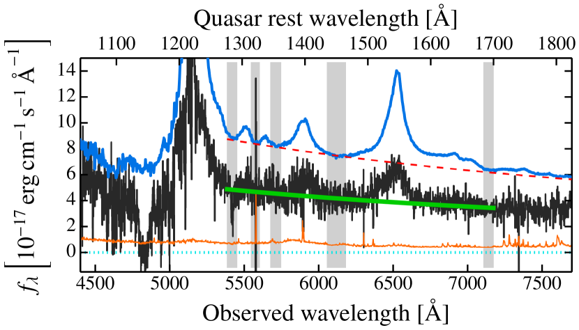
Figure 2: Example of spectral index fitting on the SDSS spectrum (black/dark solid line) of quasar J112820.20$+$325918.9 ($z_{\textrm{\scriptsize em}}=3.22$) which has a DLA at $z_{\textrm{\scriptsize abs}}=2.909$ with $\log(N_{\textsc{h\scriptsize{\,i}}}/\textrm{cm}^{-2})=20.6$ (Noterdaeme et al., 2009b). The power-law (green/grey thick line) was fitted to the median fluxes within the grey shaded regions and has a spectral index $\beta=-1.22$. The orange/thin lower line is the 1-$\sigma$ flux uncertainty. The blue/upper curve shows the median composite SDSS quasar spectrum of Vanden Berk et al. (2001) and their power-law estimate of the underlying continuum (dashed line, $\beta=-1.56$). Note that the grey shaded fitting regions are chosen to match areas of little or no quasar line emission.

For each quasar, the median flux density was determined in 5 small spectral regions (grey shaded regions in Figure 2) at quasar rest-frame wavelengths of 1276–1292, 1314–1328, 1345–1362, 1435–1465, 1684–1700 Å. As shown in Figure 2, the composite SDSS spectrum of Vanden Berk et al. (2001) in these regions shows little or no evidence for contamination from quasar line emission and is consistent with representing the underlying power-law quasar continuum. Using the median $f_{\lambda}$ value in each region provides robustness against the effects of narrow absorption features, bad pixels, residuals from the removal of telluric features and/or other narrow artefacts. The second region (1314–1328 Å) is the narrowest, but still comprises 47 SDSS pixels (69 $\textrm{km\,s}^{-1}$ pix^-1), so the median is substantially effective in guarding against these effects. As a measure of the relative uncertainty in the median fluxes, we also calculate the semi-interquartile range, i.e. half the range around the median containing half of the $f_{\lambda}$ values, in each region. These will be small for high SNR spectra and larger for low SNR spectra and/or regions that contain some features/artefacts extending over more than $\sim$10 pixels.

We estimated $\beta$ using a weighted power-law fit to these median $f_{\lambda}$ values with the inverse-squares of their semi-interquartile ranges as weights. This provides a robust, naturally-weighted $\beta$ estimate with a representative uncertainty, $\delta\beta$. These uncertainties have a median of 0.13, with semi-interquartile range of 0.05 and no strong redshift dependence. Figure 3 shows the distribution of $\beta$ with redshift for the DLA quasars and non-DLA quasars (the latter is the pool from which control quasars are selected). Note that $\beta$ evolves little with redshift in the DR7 quasar spectra. Relative to the $\beta$ distribution of the non-DLA quasars, there appears to be a small shift in the DLA quasar $\beta$ distribution to redder colours at most redshifts. This is an indication that the DLAs cause their quasars to be reddened with respect to non-DLA quasars at similar redshifts (whose spectra had sufficient SNR for those DLAs to be detected). The reddening effect is substantially smaller than the width of the $\beta$ distribution itself, highlighting the need for large statistical samples of both DLA and non-DLA quasars.

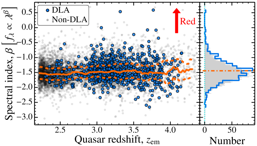
Figure 3: Distribution of spectral index, $\beta$, for the DLA quasars (dark, circled points) and non-DLA quasars (light grey points) with emission redshift. The DLA distribution clearly follows the shape of the non-DLA distribution closely. A running median (over 201 quasars) of the non-DLA quasar $\beta$ values is plotted as an orange/grey solid line and shows some evolution with redshift (the dashed lines mark the running upper and lower quartiles). The overall $\beta$ distributions are shown in the histograms (right-hand panel). The two distributions are similar and both display a skew towards redder $\beta$ values. The dot-dashed line shows the mean $\beta$ for the DLA quasars.

One potential concern with our spectral fitting procedure is that the relative weights of the different fitting regions will change with redshift. In particular, the redder fitting regions will move into noisier parts of the spectrum at higher redshifts, so they will contribute less to the weighted power-law fit to determine $\beta$. In principle, this may introduce a redshift-dependency in the spectral index results. To check this we determined the spectral index with an unweighted fit, $\beta_{\rm unweighted}$, and analysed the difference, $\beta-\beta_{\rm unweighted}$, for DLA quasars and non-DLA quasars as a function of redshift. There is no significant difference between the weighted and unweighted $\beta$ values up to $z_{\textrm{\scriptsize em}}\approx 3.3$, but above this redshift $\beta$ is smaller than $\beta_{\rm unweighted}$ by $\approx$0.1 on average. However, most importantly, this behaviour is the same for both the DLA and non-DLA samples, i.e. there is no significant differential changes between the DLA quasar and non-DLA quasar samples with redshift. It is important to realise that variations in $\beta$ – either real or spurious – over redshift intervals greater than the $\Delta z=0.1$ bin size for selecting control quasars, will not affect the $\Delta\beta$ value for a given DLA quasar. We conclude that the weighted approach to determining the spectral index of each quasar spectrum is robust, at least to the precision required for the differential reddening analysis here.

If DLAs contain negligible dust, the distribution of $\beta$ for DLA quasars and their control quasars should be indistinguishable. Significant DLA dust reddening should increase a DLA quasar’s spectral index, $\beta_{\rm DLA}$, relative to the $\beta$ distribution of its control quasars. That is, we should seek to measure

$$\Delta\beta\equiv\beta_{\rm DLA}-\left<\beta_{\rm control}\right>\,$$ (4)

for each DLA using some appropriate definition of $\left<\beta_{\rm control}\right>$, a statistic representing the $\beta$ distribution of that DLA quasar’s control sample. Figure 3 shows that the $\beta$ distribution of non-DLA quasars is non-Gaussian and asymmetric. However, it also shows that the $\beta_{\rm DLA}$ distribution has a very similar shape. We therefore make the simple assumption in our analysis that the two distributions differ only by an average shift in the $\beta$ distribution. This implies that $\left<\beta_{\rm control}\right>$ in Equation (4) is just the simple mean $\beta$ of the control sample for each DLA quasar. For example, consider the limiting case of no DLA reddening: $\beta_{\rm DLA}$ in Equation (4) is then equivalent to a single value drawn from the $\beta_{\rm control}$ distribution; considering many realizations of the same DLA quasar, the mean $\Delta\beta$ will be zero only when $\left<\beta_{\rm control}\right>$ is the mean $\beta$ of the control sample. Simple Monte Carlo experiments confirm this, using a variety of underlying $\beta$ distributions, even highly asymmetric ones, as long as statistical DLA reddening is assumed to simply shift the $\beta$ distribution of non-DLA quasars.

The above approach allows us to measure a value of $\Delta\beta$ for every DLA quasar, though it must be emphasised that individual $\Delta\beta$ measurements are not particularly meaningful and that a statistical $\Delta\beta$ distribution is needed to infer the average dust content of DLAs. One advantage of this approach is that some heavily reddened DLA quasars might be identifiable in this analysis. It also enables a simple conversion between $\Delta\beta$ and the (physically more interesting) colour excess, $E(B\!-\!V)$, using different dust extinction laws (e.g. SMC and LMC) for each DLA – see below. A more sophisticated definition of $\left<\beta_{\rm control}\right>$ might incorporate the $\beta$ uncertainties, $\delta\beta$, for the individual control quasars. However, this is only likely to affect the results if $\delta\beta$ is a strong function of $\beta$; we do not observe such a relationship in our spectral fitting results, so we use the simple mean for $\left<\beta_{\rm control}\right>$.

Finally, for each DLA quasar, we convert the $\Delta\beta$ measurement from Equation (4) into DLA rest-frame colour excess value, $E(B\!-\!V)_{\textrm{\scriptsize SMC}}$ for SMC-like dust. We redden and de-redden the DLA quasar spectrum with a wide range of $E(B\!-\!V)$ values (both positive and negative, respectively), applied in the rest-frame of the DLA, and re-measure $\beta$ for each value to establish a one-to-one relationship between $E(B\!-\!V)$ and changes in $\beta$. Interpolating this relationship then allows conversion of an arbitrary $\Delta\beta$ measurement into a $E(B\!-\!V)_{\textrm{\scriptsize SMC}}$ value for that DLA quasar. The same approach is used to derive a colour excess value for LMC-like dust, $E(B\!-\!V)_{\textrm{\scriptsize LMC}}$. We use the SMC and LMC extinction laws from Pei (1992, specifically the fitting formulae in their table 4) for this conversion. The previous spectral stacking analyses of SDSS DLAs have shown no significant evidence for a 2175 Å dust bump (Frank & Péroux, 2010; Khare et al., 2012), so we do not include a Milky Way dust law in our analysis.

4 Results

The main numerical results of this work are summarized in Table 5 and detailed in the following subsections. Correlations and linear relationships between the measured quantities – i.e. $\Delta\beta$ and $E(B\!-\!V)$ using SMC and LMC dust models – and $z_{\textrm{\scriptsize abs}}$, $N_{\textsc{h\scriptsize{\,i}}}$, metal-line equivalent widths etc. are derived using the individual measurements, while binned measurements are plotted in the main figures. Because the scatter in the $\Delta\beta$ and $E(B\!-\!V)$ measurements is completely dominated by the underlying diversity of $\beta$ values (see Figure 3), the linear relationships are derived using unweighted linear least-squares fits. The 68 per cent confidence intervals for the parameters of these relationships and the binned measurements were all calculated using a simple bootstrap method: 10⁴ bootstrap samples were formed by drawing, with replacement, random values from the observed distribution, and the distribution of the mean in the bootstrap samples provided the confidence intervals. Table 5 also presents results from Spearman rank (i.e. non-parametric) correlation tests between the parameters of interest, including the correlation coefficient, $r$, and probability, $p$, of the observed correlation being due to chance under the null hypothesis of no correlation.

Table 5: Main numerical results for correlation tests and linear fits between the individual $E(B\!-\!V)$ values, measured in milli-magnitudes (mmag), and absorption redshift ($z_{\textrm{\scriptsize abs}}$), neutral hydrogen column density ($N_{\textsc{h\scriptsize{\,i}}}$), the Si ii $\lambda$1526 rest-frame equivalent width [$W_{\textrm{\scriptsize r}}(\textrm{Si\,{{ii}}}\,\lambda{1526})$], the corresponding Si ii metallicity ($Z_{\rm Si}$) and column density ($N_{\rm Si\textsc{\scriptsize{\,ii}}}$) derived using known scaling relations (for DLAs only; see Section 4.4), and the C ii equivalent width [$W_{\textrm{\scriptsize r}}(\textrm{C\,{{ii}}}\,\lambda{1334})$]. The correlations and fits are performed for both SMC and LMC-like dust models using both the DLA sample and absorber sample [which includes sub-DLAs with $\log(N_{\textsc{h\scriptsize{\,i}}}/\textrm{cm}^{-2})\geq 20.0$]. The first column describes the ‘model’ being tested or fitted in each row. The Spearman rank correlation coefficient, $r$, and associated probability, $p$, are provided for the correlation tests.

$E(B\!-\!V)$ [mmag]	DLAs: $\log(N_{\textsc{h\scriptsize{\,i}}}/\textrm{cm}^{-2})\geq 20.3$			All absorbers: $\log(N_{\textsc{h\scriptsize{\,i}}}/\textrm{cm}^{-2})\geq 20.0$
Model	SMC dust	LMC dust		SMC dust	LMC dust
$\left<E(B\!-\!V)\right>$	$3.0\pm 1.0$	$6.2\pm 2.2$		$3.6\pm 0.9$	$7.2\pm 1.9$
$z_{\textrm{\scriptsize abs}}$ corr. test	$r=-0.03$, $p=0.35$	$r=-0.03$, $p=0.40$		$r=-0.00$, $p=0.99$	$r=-0.01$, $p=0.87$
$a+b\,z_{\textrm{\scriptsize abs}}$	$a=8.0\pm 7.8$,	$a=11\pm 19$,		$a=3.5\pm 7.0$,	$a=5\pm 17$,
	$b=-1.7\pm 2.8$	$b=-1.9\pm 7.0$		$b=0.0\pm 2.4$	$b=0.7\pm 6.2$
$N_{\textsc{h\scriptsize{\,i}}}$ corr. test	$r=0.04$, $p=0.24$	$r=0.05$, $p=0.21$		$r=0.02$, $p=0.51$	$r=0.02$, $p=0.43$
$b\,[N_{\textsc{h\scriptsize{\,i}}}/{\rm cm}^{-2}]$	$b=(3.5\pm 1.0)\times 10^{-21}$	$b=(7.8\pm 2.1)\times 10^{-21}$		$b=(3.8\pm 1.0)\times 10^{-21}$	$b=(8.3\pm 2.1)\times 10^{-21}$
$a+b\,[N_{\textsc{h\scriptsize{\,i}}}/{\rm cm}^{-2}]$	$a=1.7\pm 1.4$,	$a=2.8\pm 3.3$,		$a=2.6\pm 1.1$,	$a=4.6\pm 2.4$,
	$b=(2.4\pm 1.4)\times 10^{-21}$	$b=(6.0\pm 3.1)\times 10^{-21}$		$b=(1.9\pm 1.3)\times 10^{-21}$	$b=(4.9\pm 2.9)\times 10^{-21}$
$W_{\textrm{\scriptsize r}}(\textrm{Si\,{{ii}}}\,\lambda{1526})$ corr. test	$r=0.19$, $p=3.9\times 10^{-4}$	$r=0.19$, $p=3.8\times 10^{-4}$		$r=0.17$, $p=3.7\times 10^{-4}$	$r=0.17$, $p=5.3\times 10^{-4}$
$b\,[W_{\textrm{\scriptsize r}}(\textrm{Si\,{{ii}}}\,\lambda{1526})/{\rm\AA}]$	$b=5.0\pm 1.4$	$b=9.2\pm 3.0$		$b=6.4\pm 1.4$	$b=12\pm 3$
$a+b\,[W_{\textrm{\scriptsize r}}(\textrm{Si\,{{ii}}}\,\lambda{1526})/{\rm\AA}]$	$a=-3.7\pm 2.2$,	$a=-11\pm 5$,		$a=-1.8\pm 2.2$,	$a=-3.8\pm 4.3$,
	$b=7.8\pm 2.2$	$b=17\pm 5$		$b=7.9\pm 2.3$	$b=16\pm 5$
$b\,Z_{\rm Si}$	$b=33\pm 9$	$b=65\pm 21$
$N_{\rm Si\textsc{\scriptsize{\,ii}}}$ corr. test	$r=0.15$, $p=4.2\times 10^{-3}$	$r=0.16$, $p=2.7\times 10^{-3}$
$b\,[N_{\rm Si\textsc{\scriptsize{\,ii}}}/{\rm cm}^{-2}]$	$b=(5.2\pm 1.3)\times 10^{-16}$	$b=(10\pm 3)\times 10^{-16}$
$W_{\textrm{\scriptsize r}}(\textrm{C\,{{ii}}}\,\lambda{1334})$ corr. test	$r=0.16$, $p=4.6\times 10^{-3}$	$r=0.16$, $p=5.7\times 10^{-3}$		$r=0.12$, $p=0.02$	$r=0.11$, $p=0.03$
$b\,[W_{\textrm{\scriptsize r}}(\textrm{C\,{{ii}}}\,\lambda{1334})/{\rm\AA}]$	$b=3.1\pm 1.3$	$b=6.4\pm 2.6$		$b=3.9\pm 1.5$	$b=6.7\pm 2.7$
$a+b\,[W_{\textrm{\scriptsize r}}(\textrm{C\,{{ii}}}\,\lambda{1334})/{\rm\AA}]$	$a=-4.2\pm 2.3$,	$a=-9.4\pm 4.8$,		$a=-2.8\pm 2.4$,	$a=-6.5\pm 5.0$,
	$b=6.0\pm 2.3$	$b=13\pm 4$		$b=5.9\pm 2.5$	$b=11\pm 5$

4.1 Shift in spectral index

The upper panel of Figure 4 shows the measurements of $\Delta\beta$ [Equation (4)] for the DLA quasars against the DLA absorption redshift. Compared to the $\beta$ values shown in Figure 3, it is immediately clear that there is no apparent redshift evolution in $\Delta\beta$. However, the distribution of $\Delta\beta$ values, shown in the histogram, has a similar non-Gaussian, asymmetric shape as the $\beta$ values, as expected.

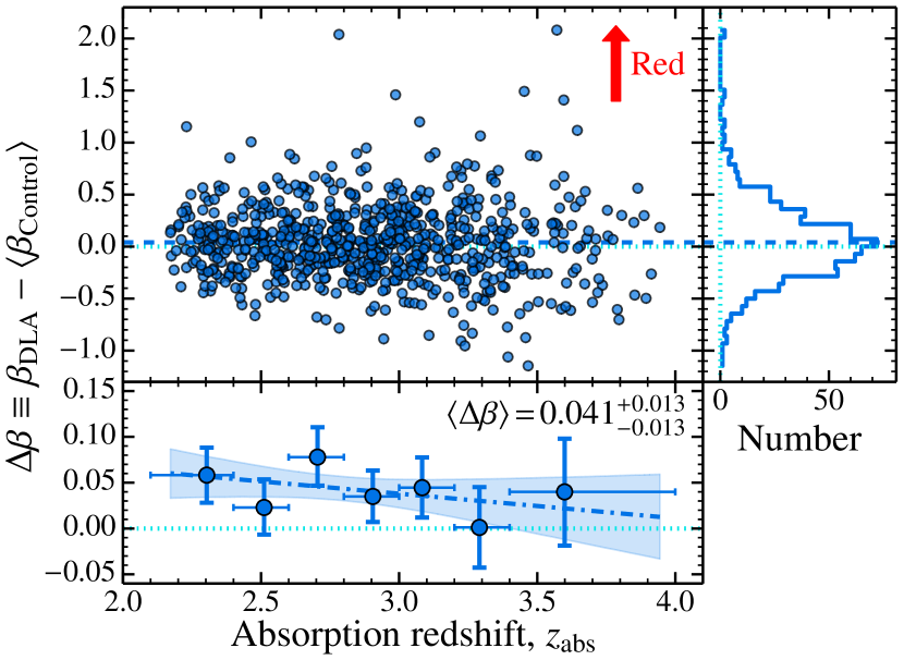
Figure 4: Distribution of the spectral index difference between the DLA quasars and their corresponding control quasar samples, $\Delta\beta$ [see Equation (4)]. The upper panels show the overall $\Delta\beta$ distribution (histogram in right-hand panel) and its relationship with absorption redshift (left-hand upper panel). The dashed line shows the mean $\Delta\beta$ value. The lower panel shows the mean $\Delta\beta$ in absorption redshift bins (defined in Figure 1) with 68 per cent bootstrap confidence intervals. The horizontal error bars indicate a bin’s redshift range and the point is plotted at the mean absorber redshift within the bin. The mean $\Delta\beta$, averaged over all redshifts (with 68 per cent confidence intervals), is also provided. The dot-dashed line is the best-fitting straight line to the individual $\Delta\beta$ values and the shaded region shows the 68 per cent bootstrap confidence region of the fit. Despite the weak redshift evolution in $\beta$ evident in Figure 3, the differential analysis used to derive $\Delta\beta$ here reveals no residual evolution in $\Delta\beta$.

The $\Delta\beta$ distribution in Figure 4 also shows that any DLA dust reddening causes a much smaller shift in $\beta$ than the typical width of the distribution. Indeed, the mean $\Delta\beta$ is only $0.041\pm 0.013$, representing some evidence for very low DLA dust reddening. The bootstrap distribution indicates that $\Delta\beta$ is $>$0 at 3.2-$\sigma$ significance; that is, the null hypothesis of no DLA dust reddening is ruled out at 99.7 per cent confidence. The lower panel of Figure 4 shows the mean $\Delta\beta$ within the absorption redshift bins defined in Figure 1. The binned results do not appear to reveal any evidence for evolution in $\Delta\beta$ with redshift. Indeed, a linear least-squares fit to the individual $\Delta\beta$ values, with bootstrap estimates of the 1-$\sigma$ parameter uncertainties, yields a best fitted relationship of $\Delta\beta=(0.12\pm 0.11)+z_{\textrm{\scriptsize abs}}\times(-0.03\pm 0.04)$, confirming this impression.

Conducting the same analysis for the absorber sample [i.e. including sub-DLAs with $\log(N_{\textsc{h\scriptsize{\,i}}}/\textrm{cm}^{-2})\geq 20.0$] yields a mean shift in the spectral index of $\Delta\beta=0.047\pm 0.012$, with $\Delta\beta>0$ at 4.8-$\sigma$ significance. That is, including the sub-DLAs somewhat increases the mean $\Delta\beta$ and substantially increases the significance of the reddening detection. As with the DLA sample, we do not find any evidence for evolution in $\Delta\beta$ with redshift.

4.2 Mean reddening and redshift evolution

Figure 5 shows the mean colour excess measurements, in the redshift bins defined in Figure 1, after converting each DLA (and absorber) quasar’s $\Delta\beta$ value to $E(B\!-\!V)_{\textrm{\scriptsize SMC}}$ and $E(B\!-\!V)_{\textrm{\scriptsize LMC}}$, as described in Section 3. The Figures and Table 5 provide the mean $E(B\!-\!V)$, averaged over all redshifts, for the DLA and absorber quasar samples in both dust models. For example, assuming DLAs contain SMC-like dust, they cause a mean colour excess of $\left<E(B\!-\!V)_{\textrm{\scriptsize SMC}}\right>=3.0\pm 1.0$ mmag over the redshift range $2<z_{\textrm{\scriptsize abs}}<4$. Assuming the dust obeys an LMC-like dust law (i.e. with a shallower extinction curve), the corresponding mean colour excess is higher, $\left<E(B\!-\!V)_{\textrm{\scriptsize LMC}}\right>=6.2\pm 2.2$ mmag. The overall evidence for $E(B\!-\!V)>0$ is, of course, very similar to that for $\Delta\beta>0$: 3.2-$\sigma$ significance, averaged over all redshifts, for both SMC and LMC-like dust.

Table 5 shows that both the colour excess and statistical significance of $E(B\!-\!V)$ increase when sub-DLAs with $\log(N_{\textsc{h\scriptsize{\,i}}}/\textrm{cm}^{-2})\geq 20.0$ are included (as also seen for $\Delta\beta$). In both dust models, $E(B\!-\!V)=0$ is ruled out at 4.8-$\sigma$ significance.

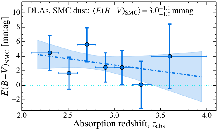
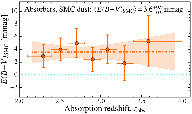
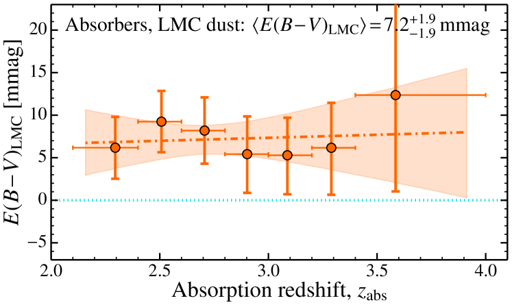
Figure 5: The mean colour excess, $E(B\!-\!V)$, in the absorber rest-frame in bins of absorption redshift (defined in Figure 1). The upper plots show the mean $E(B\!-\!V)_{\textrm{\scriptsize SMC}}$ (left-hand plot) and $E(B\!-\!V)_{\textrm{\scriptsize LMC}}$ (right-hand plot) values for the DLAs, while the lower plots show the values for all absorbers with $\log(N_{\textsc{h\scriptsize{\,i}}}/\textrm{cm}^{-2})\geq 20.0$. Note the doubled $E(B\!-\!V)$ scale for the LMC plots. The vertical error bars represent the 68 per cent bootstrap confidence intervals. The horizontal error bars indicate a bin’s range and the point is plotted at the mean absorber redshift within the bin. The dot-dashed lines are the best-fit straight lines to the individual $E(B\!-\!V)$ values as a function of redshift, with the 68 per cent bootstrap confidence intervals in the fits shown as shaded regions.

Figure 5 reveals no evidence for redshift evolution in the colour excess caused by dust in DLAs and sub-DLAs. The bootstrap uncertainty in the (assumed) linear relationship between $E(B\!-\!V)$ and $z_{\textrm{\scriptsize abs}}$ is illustrated by the shaded regions in the Figures; these are all clearly consistent with no evolution in $E(B\!-\!V)$. The best-fit parameter values and uncertainties are provided in Table 5. For example, the 1-$\sigma$ limit on evolution in $E(B\!-\!V)_{\textrm{\scriptsize SMC}}$ is 2.8 mmag per unit redshift for DLAs, assuming an SMC-like dust model, and a similar value, 2.4 mmag per redshift interval, when including sub-DLAs. The lack of redshift evolution is also confirmed in Table 5 with the Spearman rank tests for correlations. These return $p$ values $>$35 per cent in all four cases (DLA and absorber samples with SMC and LMC-like dust), indicating no significant correlation between $E(B\!-\!V)$ and $z_{\textrm{\scriptsize abs}}$. Over the same redshift interval, $z_{\textrm{\scriptsize abs}}=4$–2, the mean DLA metallicity has been found to increase by a factor of $\approx$2.5 (Rafelski et al., 2012; Jorgenson et al., 2013). If the mean dust column scales linearly with DLA metallicity, as expected in simple models (e.g. Vladilo & Péroux, 2005), we should expect a slope of $b\approx 1.3$ mmag per unit redshift in $E(B\!-\!V)_{\textrm{\scriptsize SMC}}$. However, Table 5 shows that our 1-$\sigma$ sensitivity to a slope is $b=2.8$ mmag per unit redshift. That is, the SDSS DLA dataset is not large enough to detect the evolution in dust content expected from the observed metallicity evolution in DLAs.

4.3 Reddening vs. neutral hydrogen column density

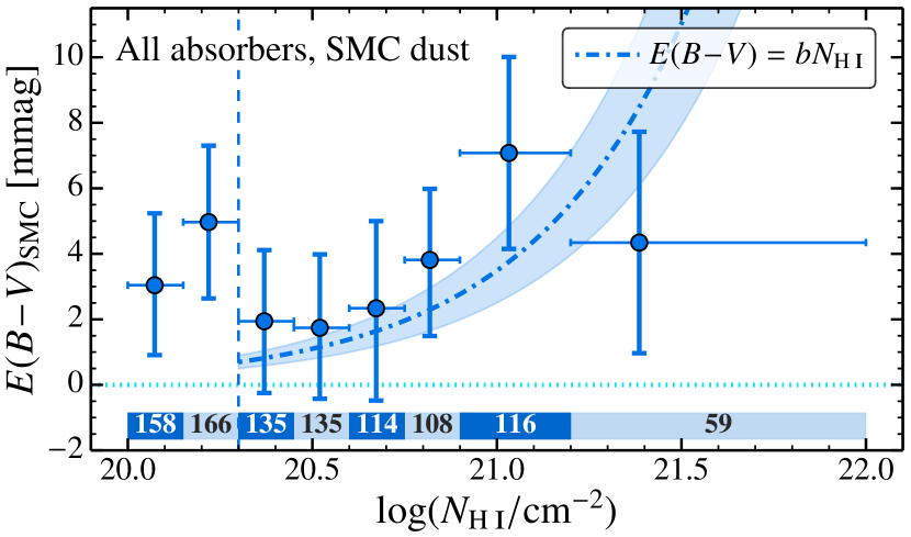
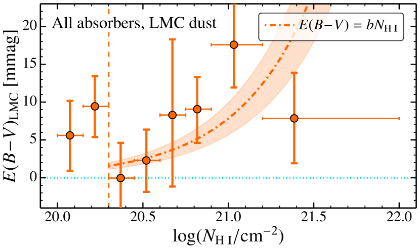
Figure 6: The mean colour excess, $E(B\!-\!V)$, in the absorber rest-frame in bins of $\log N_{\textsc{h\scriptsize{\,i}}}$. The upper plot shows the mean $E(B\!-\!V)_{\textrm{\scriptsize SMC}}$ values while the lower plot shows the $E(B\!-\!V)_{\textrm{\scriptsize LMC}}$ values. Note the doubled $E(B\!-\!V)$ scale for the LMC plot. The shaded bar in the upper plot shows the number of absorbers in each $\log N_{\textsc{h\scriptsize{\,i}}}$ bin. The vertical error bars represent the 68 per cent bootstrap confidence intervals. The horizontal error bars indicate a bin’s range and the point is plotted at the mean $\log N_{\textsc{h\scriptsize{\,i}}}$ within the bin. The dot-dashed lines are the best-fit straight lines to the individual $E(B\!-\!V)$ values as a function of $N_{\textsc{h\scriptsize{\,i}}}$ [not $\log N_{\textsc{h\scriptsize{\,i}}}$, hence their curvature in the plot], with the 68 per cent bootstrap confidence intervals in the fits shown as shaded regions. The dashed lines delineate DLAs and sub-DLAs. Note that the results in both plots were derived from analysing the absorber (and corresponding non-absorber) sample containing DLAs and sub-DLAs with $\log(N_{\textsc{h\scriptsize{\,i}}}/\textrm{cm}^{-2})\geq 20.0$. The results from the DLA/non-DLA analysis are very similar for $\log(N_{\textsc{h\scriptsize{\,i}}}/\textrm{cm}^{-2})\geq 20.3$.

Figure 6 shows the mean colour excess measurements in bins of $\log N_{\textsc{h\scriptsize{\,i}}}$ using the sample of all absorbers with $\log(N_{\textsc{h\scriptsize{\,i}}}/\textrm{cm}^{-2})\geq 20.0$. Using the DLA sample returns very similar results at $\log(N_{\textsc{h\scriptsize{\,i}}}/\textrm{cm}^{-2})\geq 20.3$ but, by definition, does not extend to lower $N_{\textsc{h\scriptsize{\,i}}}$, so we focus on the full absorber sample here. The binned results in Figure 6 provide no evidence for strong variations in $E(B\!-\!V)$ with increasing $N_{\textsc{h\scriptsize{\,i}}}$. Nor do the Spearman rank correlation tests in Table 5 indicate significant correlation or anti-correlation ($p>0.2$ in all cases). It is instead notable that the amount of reddening is similar at all H i column densities over a 1.5 order-of-magnitude range and that the highest and lowest $N_{\textsc{h\scriptsize{\,i}}}$ bins show no discernable differences.

In both the SMC and LMC, the colour excess is correlated with $N_{\textsc{h\scriptsize{\,i}}}$, with the reddening per H atom (including contributions from H₂) being $E(B\!-\!V)/N_{\rm H}\approx 2\times 10^{-23}$ (Martin et al., 1989) and ${\approx}4.5\times 10^{-23}$ mag cm² (Fitzpatrick, 1985), respectively. This motivates a linear fit between our individual $E(B\!-\!V)$ results and $N_{\textsc{h\scriptsize{\,i}}}$, as shown by the dot-dashed lines and 1-$\sigma$ shaded regions in Figure 6. Although there is no evidence for such a relationship, as discussed above, the data in Figure 6 are not inconsistent with the best-fit relationships derived. For better comparison with the SMC and LMC, we restricted these fits to DLAs according to the traditional threshold for selecting only the most neutral absorbers [i.e. $\log(N_{\textsc{h\scriptsize{\,i}}}/\textrm{cm}^{-2})\geq 20.3$]. The resulting parameter estimates are given in Table 5. Assuming a negligible H₂ molecular fraction in our DLAs, the mean reddening per H atom is $E(B\!-\!V)_{\textrm{\scriptsize SMC}}/N_{\rm H}\approx 0.4\times 10^{-23}$ and $E(B\!-\!V)_{\textrm{\scriptsize LMC}}/N_{\rm H}\approx 0.8\times 10^{-23}$ cm². These are only $\approx$20 per cent of the SMC and LMC values given above.

Even if the assumption of a simple linear relationship between $E(B\!-\!V)$ and $N_{\textsc{h\scriptsize{\,i}}}$ is valid for DLAs, the much smaller mean reddening per H atom for DLAs is most likely explained by their much lower average metallicity of $\sim$1/30 solar (e.g. Rafelski et al., 2012; Jorgenson et al., 2013) compared to the SMC and LMC ($\sim$1/7 and $\sim$1/3 solar; Kurt & Dufour, 1998; Draine, 2003). However, while the interstellar medium within each of the Magellanic Clouds shows little metallicity variation, the DLA population exhibits a very large range, $\left[\textrm{M}/\textrm{H}\right]\sim-3.0$–0.0. Therefore, even if $E(B\!-\!V)$ correlates tightly with $N_{\textsc{h\scriptsize{\,i}}}$ in the different regions of individual high-redshift galaxies (e.g. disk, gaseous halo etc.) with $\log(N_{\textsc{h\scriptsize{\,i}}}/\textrm{cm}^{-2})\geq 20.3$, the large metallicity range of the DLAs – an ensemble of different regions from different galaxies – will tend to flatten any $E(B\!-\!V)$ vs. $N_{\textsc{h\scriptsize{\,i}}}$ correlation, possibly leading to an apparently flat relationship like those observed in Figure 6.

4.4 Reddening vs. metal line equivalent width, metallicity and metal column density

In addition to measuring $N_{\textsc{h\scriptsize{\,i}}}$ for each DLA candidate, Noterdaeme et al. (2009b) determined the equivalent widths of several strong metal absorption lines when they fell redwards of the quasar $\textrm{Ly-}\alpha$ emission line. Si ii $\lambda$1526 is the strongest Si ii transition and its rest-frame equivalent width, $W_{\textrm{\scriptsize r}}(\textrm{Si\,{{ii}}}\,\lambda{1526})$, was reported for 355 of the 730 DLA quasars in our statistical analysis (and 428 of the 991 absorber quasars). Similarly, $W_{\textrm{\scriptsize r}}(\textrm{C\,{{ii}}}\,\lambda{1334})$ was reported for 303 DLA quasars (and 373 absorber quasars). The unreported cases will be a mix of non-detections (i.e. where the metal absorption was too weak to detect) and where detection was precluded, either because the transitions fell bluewards of the quasar $\textrm{Ly-}\alpha$ emission line or due to some artefact in the spectra (e.g. bad pixels).

Figures 7 and 8 show the mean colour excess measurements in bins of $W_{\textrm{\scriptsize r}}(\textrm{Si\,{{ii}}}\,\lambda{1526})$ and $W_{\textrm{\scriptsize r}}(\textrm{C\,{{ii}}}\,\lambda{1334})$, respectively. There is a clear tendency for systems with larger metal-line equivalent widths to exhibit more reddening. The correlation tests in Table 5 confirm this: for example, $E(B\!-\!V)_{\textrm{\scriptsize SMC}}$ correlates strongly with $W_{\textrm{\scriptsize r}}(\textrm{Si\,{{ii}}}\,\lambda{1526})$ for DLAs, with the Spearman rank test giving a probability of $p=0.04$ per cent of the observed level of correlation occurring by chance alone, i.e. a $\approx$3.5-$\sigma$ significance. The correlation is of similar strength, but lower significance ($\approx$2.8 $\sigma$), between $E(B\!-\!V)_{\textrm{\scriptsize SMC}}$ and $W_{\textrm{\scriptsize r}}(\textrm{C\,{{ii}}}\,\lambda{1334})$. Figures 7 and 8 also show the best linear fits to the ensemble of $E(B\!-\!V)$ and metal-line equivalent width measurements from individual absorbers. Table 5 provides the best-fitting parameters: for example, $E(B\!-\!V)_{\textrm{\scriptsize SMC}}=(5.0\pm 1.4)\times[W_{\textrm{\scriptsize r}}(\textrm{Si\,{{ii}}}\,\lambda{1526})/$Å$]$ mmag for DLAs.

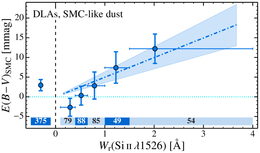
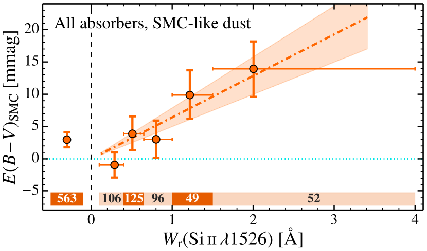
Figure 7: The mean colour excess for SMC-like dust, $E(B\!-\!V)_{\textrm{\scriptsize SMC}}$, in the absorber rest-frame in bins of Si ii $\lambda$1526 rest equivalent width, $W_{\textrm{\scriptsize r}}(\textrm{Si\,{{ii}}}\,\lambda{1526})$. The upper plot shows the mean $E(B\!-\!V)_{\textrm{\scriptsize SMC}}$ values for the DLAs, while the lower plot shows the values for all absorbers with $\log(N_{\textsc{h\scriptsize{\,i}}}/\textrm{cm}^{-2})\geq 20.0$. The shaded bar in each plot shows the number of absorbers in each bin. The left-most point in each plot is the mean $E(B\!-\!V)$ value for DLAs/absorbers in which Si ii was not detected (see main text). The vertical error bars represent the 68 per cent bootstrap confidence intervals. The horizontal error bars indicate a bin’s range and the point is plotted at the mean $W_{\textrm{\scriptsize r}}(\textrm{Si\,{{ii}}}\,\lambda{1526})$ within the bin. The dot-dashed lines are the best-fit straight lines to the individual $E(B\!-\!V)$ values as a function of $W_{\textrm{\scriptsize r}}(\textrm{Si\,{{ii}}}\,\lambda{1526})$, with the 68 per cent bootstrap confidence intervals in the fits shown as shaded regions.

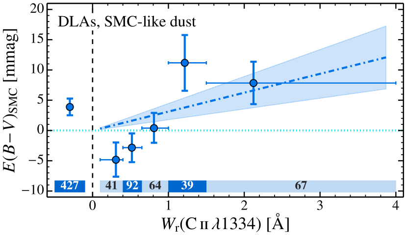
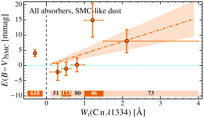
Figure 8: The mean colour excess for SMC-like dust, $E(B\!-\!V)_{\textrm{\scriptsize SMC}}$, in the absorber rest-frame in bins of C ii $\lambda$1334 rest equivalent width, $W_{\textrm{\scriptsize r}}(\textrm{C\,{{ii}}}\,\lambda{1334})$. The upper plot shows the mean $E(B\!-\!V)_{\textrm{\scriptsize SMC}}$ for DLAs while the lower plot shows the values for all absorbers with $\log(N_{\textsc{h\scriptsize{\,i}}}/\textrm{cm}^{-2})\geq 20.0$. The shaded bars show the number of absorbers in each bin. The left-most point in each plot is the mean $E(B\!-\!V)_{\textrm{\scriptsize SMC}}$ value for DLAs/absorbers in which C ii was not detected (see main text). The vertical error bars represent the 68 per cent bootstrap confidence intervals. The horizontal error bars indicate a bin’s range and the point is plotted at the mean $W_{\textrm{\scriptsize r}}(\textrm{C\,{{ii}}}\,\lambda{1334})$ within the bin. The dot-dashed lines are the best-fit straight lines to the individual $E(B\!-\!V)_{\textrm{\scriptsize SMC}}$ values as a function of $W_{\textrm{\scriptsize r}}(\textrm{C\,{{ii}}}\,\lambda{1334})$, with the 68 per cent bootstrap confidence intervals in the fits shown as shaded regions.

A strong correlation between DLA dust content and metal-line column density is perhaps the most basic and assumption-free relationship we should expect (e.g. Vladilo & Péroux, 2005). Given the SDSS spectral resolution of $\sim$170 $\textrm{km\,s}^{-1}$ and the typical rest-frame equivalent width detection limits ($\sim$0.15 Å at 1-$\sigma$), the detected metal transitions will be predominantly saturated. Therefore, variation in their equivalent widths will more directly reflect variations in the total velocity width of the underlying absorption profile – i.e. the velocity spread amongst the individual $\sim$5–10-$\textrm{km\,s}^{-1}$-wide components – rather than the metal column densities of those individual components. Nevertheless, a broader profile will in general comprise more components, so the metal column density should correlate strongly with equivalent width. That is, we should expect the dust column density and $E(B\!-\!V)$ to correlate strongly with $W_{\textrm{\scriptsize r}}(\textrm{Si\,{{ii}}}\,\lambda{1526})$ and $W_{\textrm{\scriptsize r}}(\textrm{C\,{{ii}}}\,\lambda{1334})$. Therefore, the increase in $E(B\!-\!V)$ with increasing metal-line equivalent width in Figs. 7 and 8 indicates that the mean reddening of DLA quasars we observe (Figure 4) is really due to dust in the DLAs and not due (primarily) to some spurious, systematic effect.

Considering all absorbers with $\log(N_{\textsc{h\scriptsize{\,i}}}/\textrm{cm}^{-2})\geq 20.0$, the correlations for $E(B\!-\!V)$ and $W_{\textrm{\scriptsize r}}(\textrm{Si\,{{ii}}}\,\lambda{1526})$ have similar strengths and significance, and the best-fit linear relationships have similar slopes, as for DLAs (assuming either SMC or LMC-like dust). However, for $W_{\textrm{\scriptsize r}}(\textrm{C\,{{ii}}}\,\lambda{1334})$, the correlation becomes weaker and substantially less significant: e.g. for SMC-like dust, the by-chance correlation probability between $E(B\!-\!V)_{\textrm{\scriptsize SMC}}$ and $W_{\textrm{\scriptsize r}}(\textrm{C\,{{ii}}}\,\lambda{1334})$ increases from $p=0.5$ per cent for the 303 DLA quasars to 2 per cent for the 373 absorber quasars. Comparison of the upper and lower panels of Figure 8, which show the $E(B\!-\!V)_{\textrm{\scriptsize SMC}}$–$W_{\textrm{\scriptsize r}}(\textrm{C\,{{ii}}}\,\lambda{1334})$ relationships for DLA and absorber quasars, indicates that the main difference is at low values of $W_{\textrm{\scriptsize r}}(\textrm{C\,{{ii}}}\,\lambda{1334})$: for DLA quasars the two lowest-$W_{\textrm{\scriptsize r}}(\textrm{C\,{{ii}}}\,\lambda{1334})$ bins lie $\approx$1.1 and 1.7-$\sigma$ below zero reddening, while for the absorber quasars they are closer to zero. That is, the strength of the $E(B\!-\!V)$–$W_{\textrm{\scriptsize r}}(\textrm{C\,{{ii}}}\,\lambda{1334})$ correlation for DLAs may be overestimated in the DLA and absorber quasar samples. While the deviation of $E(B\!-\!V)$ below zero at low $W_{\textrm{\scriptsize r}}(\textrm{C\,{{ii}}}\,\lambda{1334})$ is consistent with a statistical fluctuation, it may indicate that we generally underestimate $E(B\!-\!V)$ in our sample. We consider one possible systematic effect that could, in principle, cause this – the SDSS colour-selection algorithm for selecting quasars for spectroscopic follow-up – in Section 5, though we conclude there that it causes $<$5 per cent bias at all redshifts in our samples.

The equivalent width of Si ii $\lambda$1526 is also particularly interesting because it has been found to correlate very strongly with DLA metallicity, [M/H], with only a $\sim$0.25 dex scatter and a linear relationship as follows (Prochaska et al., 2008):

$$[{\rm M}/{\rm H}]=(-0.92\pm 0.05)+(1.41\pm 0.10)\log_{10}[W_{\textrm{\scriptsize r}}(\textrm{Si\,{{ii}}}\,\lambda{1526})/{\rm\AA}]\,.$$ (5)

Similarly tight and strong relationships were also reported by Kaplan et al. (2010), Neeleman et al. (2013) and Jorgenson et al. (2013). The upper panel of Figure 9 shows the result of converting $W_{\textrm{\scriptsize r}}(\textrm{Si\,{{ii}}}\,\lambda{1526})$ to metallicity using Equation (5) for the DLAs and the linear fit between $E(B\!-\!V)_{\textrm{\scriptsize SMC}}$ and $W_{\textrm{\scriptsize r}}(\textrm{Si\,{{ii}}}\,\lambda{1526})$ from Figure 7’s upper panel. Table 5 also shows the results for the best linear fits between the ensemble of $E(B\!-\!V)$ values for DLAs and $Z_{\rm Si}\equiv 10^{[{\rm M}/{\rm H}]}$ derived using Equation (5); for example, $E(B\!-\!V)_{\textrm{\scriptsize SMC}}=(33\pm 9)\,Z_{\rm Si}$ mmag. By comparison, assuming that $E(B\!-\!V)$ is instead linearly proportional to $W_{\textrm{\scriptsize r}}(\textrm{Si\,{{ii}}}\,\lambda{1526})$, Equation (5) implies that $E(B\!-\!V)$ should be proportional to $Z_{\rm Si}^{1/1.41}$; for example, from the fitting results in Table 5 for SMC-like dust in DLAs, the relationship would be $E(B\!-\!V)_{\textrm{\scriptsize SMC}}=(23\pm 6)\,Z_{\rm Si}^{1/1.41}$ mmag. While both relationships appear to reasonably reflect the underlying trend between $E(B\!-\!V)$ and metal-line equivalent width and/or metallicity that we observe, the significant scatter in our $E(B\!-\!V)$ values clearly prevents us from assessing which relationship is a more accurate description.

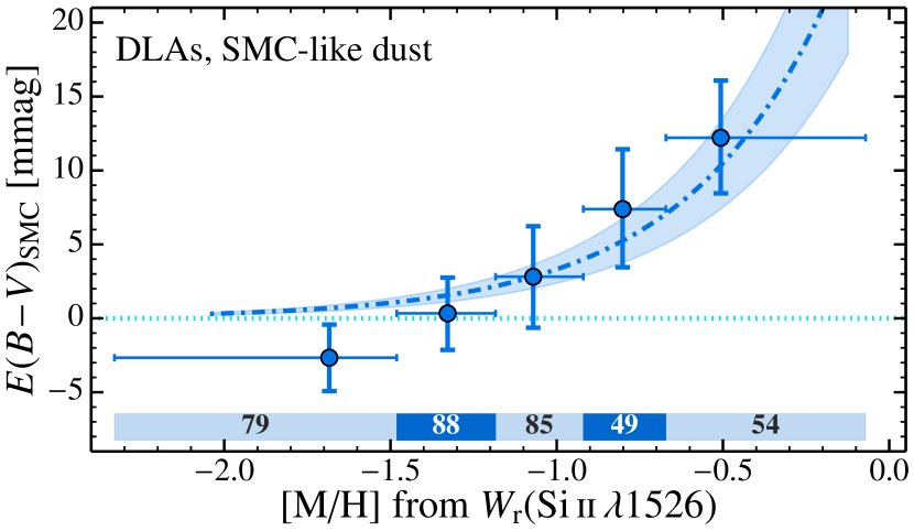
Figure 9: Relationship between mean colour-excess for SMC-like dust in DLAs and the metallicity, [M/H], and Si ii column density, $N_{\rm Si\textsc{\scriptsize{\,ii}}}$, inferred from $W_{\textrm{\scriptsize r}}(\textrm{Si\,{{ii}}}\,\lambda{1526})$ and $N_{\textsc{h\scriptsize{\,i}}}$. The upper panel shows $E(B\!-\!V)_{\textrm{\scriptsize SMC}}$ in bins of [M/H] and the best-fitted linear relationship between $E(B\!-\!V)_{\textrm{\scriptsize SMC}}$ and $W_{\textrm{\scriptsize r}}(\textrm{Si\,{{ii}}}\,\lambda{1526})$ (dot-dashed line), both converted to metallicity using the known, tight correlation between $W_{\textrm{\scriptsize r}}(\textrm{Si\,{{ii}}}\,\lambda{1526})$ and [M/H] in DLAs in Equation (5). The shaded bars show the number of absorbers in each bin. DLAs for which $W_{\textrm{\scriptsize r}}(\textrm{Si\,{{ii}}}\,\lambda{1526})$ was not reported by Noterdaeme et al. (2009b) are excluded. The vertical error bars represent the 68 per cent bootstrap confidence intervals. The horizontal error bars indicate a bin’s range and the point is plotted at the mean [M/H] within the bin. The lower panel shows the same information for bins of $N_{\rm Si\textsc{\scriptsize{\,ii}}}$ derived from $W_{\textrm{\scriptsize r}}(\textrm{Si\,{{ii}}}\,\lambda{1526})$ using Equation (5) and the $N_{\textsc{h\scriptsize{\,i}}}$ value for each DLA. The dot-dashed line shows the best-fit straight line to the individual $E(B\!-\!V)_{\textrm{\scriptsize SMC}}$ values as a function of $N_{\rm Si\textsc{\scriptsize{\,ii}}}$, with the 68 per cent bootstrap confidence interval in the fit shown as a shaded region.

The lower panel of Figure 9 shows the result of converting $W_{\textrm{\scriptsize r}}(\textrm{Si\,{{ii}}}\,\lambda{1526})$ to a Si ii column density using Equation (5) and the neutral hydrogen column density for each DLA, i.e. $N_{\rm Si\textsc{\scriptsize{\,ii}}}=10^{-0.92}\left[N_{\rm Si\textsc{\scriptsize{\,ii}}}/N_{\textsc{h\scriptsize{\,i}}}\right]_{\odot}W_{\textrm{\scriptsize r}}(\textrm{Si\,{{ii}}}\,\lambda{1526})^{1.41}N_{\textsc{h\scriptsize{\,i}}}$. Table 5 shows that, while a correlation between $E(B\!-\!V)$ and $N_{\rm Si\textsc{\scriptsize{\,ii}}}$ is apparent, the statistical significance is lower than that between $E(B\!-\!V)$ and $W_{\textrm{\scriptsize r}}(\textrm{Si\,{{ii}}}\,\lambda{1526})$. For example, $E(B\!-\!V)_{\textrm{\scriptsize SMC}}$ is correlated with $W_{\textrm{\scriptsize r}}(\textrm{Si\,{{ii}}}\,\lambda{1526})$ at $\approx$3.5-$\sigma$ but only at $\approx$2.8-$\sigma$ with the values of $N_{\rm Si\textsc{\scriptsize{\,ii}}}$ derived in this way. This is likely due to the lack of any strong correlation between $E(B\!-\!V)$ and $N_{\textsc{h\scriptsize{\,i}}}$ in our sample (see Figure 6 and Table 5). The best-fitted linear relationship between the individual $E(B\!-\!V)$ measurements and the $N_{\rm Si\textsc{\scriptsize{\,ii}}}$ values is provided in Table 5 and, for SMC-like dust in DLAs, plotted in Figure 9. The reduced significance of the correlation is apparent, with a larger scatter around the best-fit relationship observed here compared to, e.g., the relationship with [M/H] in the upper panel.

5 Magnitude and colour selection biases

Dust in DLAs will cause both extinction and reddening of DLA quasars. Therefore, it is important to address the possible effect that the magnitude and colour-selection criteria of SDSS quasars (Richards et al., 2002) may have on the measured reddening signal. Dusty DLAs may be preferentially selected or rejected, with the degree of bias varying with redshift. This possibility has not been thoroughly addressed in previous SDSS DLA reddening studies, possibly because the selection algorithm is very complex and not available in portable, public software. The colour-selection criteria are highly redshift-dependent, especially around redshifts where optical quasar colours are very similar to stellar colours, $z_{\textrm{\scriptsize em}}\sim 2.5$–3.0, which is especially concerning for reddening studies of DLAs. The magnitude selection criterion for most SDSS quasar candidates ($i\leq 19.1$ mag) is, by comparison, relatively simple and, being applied in the $i$-band, will be less affected by dust extinction than the bluer $u$, $g$ and $r$ bands. However, the effect of dust on the $i$-band magnitude will increase as the absorber redshift increases. Further, a fainter magnitude criterion of $i<20.2$ mag was applied to candidates which, from the photometric colours, indicated the quasar was likely at high redshift, $z_{\textrm{\scriptsize em}}>3.0$.

To address this concern and test the potential biases on our $E(B\!-\!V)$ measurements, we have emulated the selection criteria for spectroscopic follow-up of SDSS quasar candidates detailed by Richards et al. (2002). Our implementation and some basic performance tests are described in Appendix A, and the code is made publicly available in a portable form in Bernet & Murphy (2015). While we hope this code has broad usefulness, we emphasise that it has been tested mainly for its purpose in the current analysis; we encourage other researchers to test it for their specific purposes. We also note that there exist several additional, practical criteria that determined whether a specific quasar candidate was followed-up spectroscopically that are not reflected in our algorithm at all. For example, “fibre collisions” between quasar candidates and higher-priority targets for the SDSS (e.g. low-$z$ galaxies) may mean that a specific quasar candidate that passed the magnitude and colour-selection criteria was not observed in reality. In this respect, our emulation of the quasar selection algorithm should only be used in a statistical way.

With the quasar selection algorithm in hand, we can artificially dust-redden each quasar spectrum, with a certain $E(B\!-\!V)$, and then check whether they are selected by the quasar algorithm. This approach enables the simple test shown in Figure 10. Here we use the entire sample of quasars in the Noterdaeme et al. (2009b) catalogue which fall in the relevant redshift range for our study, $2.2\leq z_{\textrm{\scriptsize em}}\leq 4.42$. This provides a 10-times larger sample than, say, applying the test to just the DLA quasar sample alone. Three different SMC-like reddening values [$E(B\!-\!V)_{\textrm{\scriptsize SMC}}=0$, 0.02 and 0.04 mag] are applied, at the emission redshift, to each quasar’s photometry and spectrum, and the resulting $ugriz$ magnitudes are passed through our selection code. Figure 10 compares the mean spectral index, $\beta$ (determined as in Section 3), as a function of emission redshift in bins containing 100 quasars, both before (black line) and after (dashed red line) the selection code is applied.

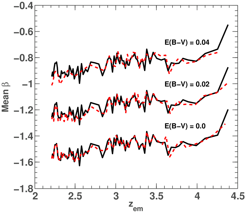
Figure 10: Mean spectral index, $\beta$, in bins containing 100 quasars, as a function of emission redshift, $z_{\textrm{\scriptsize em}}$, for the 7929 quasars in the Noterdaeme et al. (2009b) sample falling in the relevant redshift range ($2.2\leq z_{\textrm{\scriptsize em}}\leq 4.42$). The black solid lines show the mean $\beta$ for the original sample [i.e. $E(B\!-\!V)_{\textrm{\scriptsize SMC}}=0$ mag] and where each quasar spectrum was reddened with $E(B\!-\!V)_{\textrm{\scriptsize SMC}}=0.02$ and 0.04 mag. The red dashed lines show the mean $\beta$ of the reduced samples after passing the appropriately reddened photometry through our emulation of the SDSS quasar selection algorithm in Appendix A.

Firstly, Figure 10 demonstrates the simple, expected result that reddening the spectra by an increment of $E(B\!-\!V)_{\textrm{\scriptsize SMC}}=0.02$ mag increases the mean $\beta$ by $\sim$0.3 over the whole redshift range. Secondly, focussing on the zero-reddening case, note that the after-selection curve (red dashed line) does not completely match the before-selection curve (black line). This is because not all quasars in the Noterdaeme et al. (2009b) catalogue are colour-selected; $\approx$9 per cent of the SDSS DR7 quasars were selected by other criteria, such as radio loudness or X-ray emission (Schneider et al., 2010). Figure 11 shows the fraction of quasars that pass the magnitude and colour-selection criteria in our code – which we refer to as the “colour-selected fraction” for brevity – is a function of $E(B\!-\!V)_{\textrm{\scriptsize SMC}}$. The colour-selected fraction at zero reddening is similar to that expected, and the fraction remaining at $E(B\!-\!V)_{\textrm{\scriptsize SMC}}=0.003$ mag – the mean value we find for SDSS DLAs – is just $\approx$2 per cent lower than at zero reddening. Nevertheless, the fraction drops very quickly with increased reddening, and just $\approx$52 per cent remain if a reddening of $E(B\!-\!V)_{\textrm{\scriptsize SMC}}=0.04$ mag is applied. See Appendix A for a description of the channels through which a quasar can escape the magnitude and colour-selection criteria.

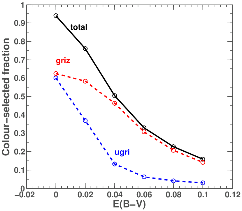
Figure 11: Fraction of quasars passing the magnitude and colour selection criteria (“colour-selected fraction”) in our emulated SDSS algorithm (Appendix A) as a function of the artificial reddening applied, $E(B\!-\!V)_{\textrm{\scriptsize SMC}}$ (at the quasar emission redshift), to the photometry. The blue (lower) and red (higher) dashed lines correspond to quasar selected via the $ugri$ (typically $z_{\textrm{\scriptsize em}}<3.0$) and $griz$ (typically $z_{\textrm{\scriptsize em}}>3.0$) channels, whereas the “total” (black solid line) corresponds to those selected via either the $ugri$ or $griz$ channels. See Appendix A for further details.

Finally and most importantly, Figure 10 clearly demonstrates that, despite the $\sim$50 per cent decrease in the colour-selected fraction at $E(B\!-\!V)_{\textrm{\scriptsize SMC}}=0.04$ mag, the mean $\beta$ is almost unaffected and, at all redshifts, is very similar to the mean $\beta$ before the magnitude and colour-selection criteria are applied. Indeed, the difference between the before- and after-selection curves for the $E(B\!-\!V)_{\textrm{\scriptsize SMC}}=0.04$ mag case is $<$5 per cent of the absolute shift in mean $\beta$ (i.e. from the zero-reddening case). The largest effects are only seen at the lowest and highest redshifts ($z_{\textrm{\scriptsize em}}\la 2.4$ and $\ga$4.4), so they will have little bearing on our DLA reddening results because the fewest DLAs are found in quasars at these emission redshifts (see Figure 1). We therefore conclude that the magnitude and colour-selection criteria for spectroscopic follow-up of SDSS quasar candidates has had a negligible effect on our reddening estimates for (sub-)DLAs.

6 Discussion

6.1 Comparison with recent DLA dust reddening measurements

Figure 12 compares our new DLA dust reddening measurement with those from the other recent studies outlined in Section 1. The six measurements shown are classified according to the methodology used: quasar spectral index measurements, as used in our work here and the early reddening limit from Murphy & Liske (2004); the distribution of quasar photometric colours, as analysed by Vladilo et al. (2008) and, very recently, Fukugita & Ménard (2015); or by analysing composite (‘stacked’) quasar spectra, as in Frank & Péroux (2010) and Khare et al. (2012). For ease of comparison, all results are cast in terms of the mean colour excess from SMC-like dust, $E(B\!-\!V)_{\textrm{\scriptsize SMC}}$, over the whole sample studied. Because all results derive from SDSS data, they all cover a similar redshift range, $2.2\la z_{\textrm{\scriptsize abs}}\la 3.5$, except Fukugita & Ménard (2015) who restrict their DR9 $(g-i)$ colour analysis to $2.1<z_{\textrm{\scriptsize abs}}<2.3$ to avoid contamination of the $g$-band photometry from $\textrm{Ly-}\alpha$ absorption. Finally, the measurements in Figure 12 are based on DLAs only, except that of Khare et al. (2012): in this case we report the $E(B\!-\!V)_{\textrm{\scriptsize SMC}}$ value from their ‘S1’ comparison of 1084 quasars with a foreground $\log(N_{\textsc{h\scriptsize{\,i}}}/\textrm{cm}^{-2})\geq 20.0$ absorber and the appropriate control sample.

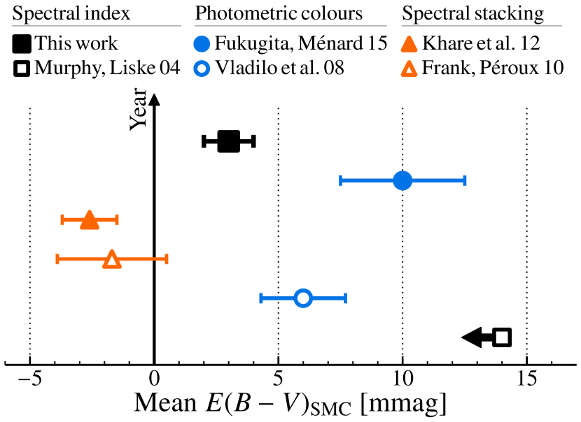
Figure 12: Summary of recent SDSS DLA dust reddening measurements, separated by methodology: analysis of spectral indices (Murphy & Liske, 2004, and the present paper), photometric colours (Vladilo et al., 2008; Fukugita & Ménard, 2015) and stacked spectra (Frank & Péroux, 2010; Khare et al., 2012). The dust reddening is characterised by the mean colour excess for SMC-like dust, $E(B\!-\!V)_{\textrm{\scriptsize SMC}}$, and 1-$\sigma$ error bars are given for all points (see text).

Figure 12 highlights the apparent disagreement between the extant measurements of $E(B\!-\!V)_{\textrm{\scriptsize SMC}}$. Our new measurement is consistent with the photometric colour analysis of Vladilo et al. (2008) at $\approx$1.1-$\sigma$, but somewhat inconsistent with the higher $E(B\!-\!V)_{\textrm{\scriptsize SMC}}$ value of $\approx$10 mmag from the colour analysis of Fukugita & Ménard (2015) (i.e. a $\approx$2.6-$\sigma$ difference). And while those two previous colour analyses are consistent with each other, they both differ significantly from the non-detection of Frank & Péroux (2010) using spectral stacking (at $\approx$2.9 and 3.5-$\sigma$, respectively) and also the negative result from Khare et al. (2012). Our result differs from these two results from spectral stacking as well. Clearly, taking all the existing measurements at face-value, there is no clear indication which, if any, indicate the correct mean dust reddening in SDSS DLAs. It is therefore worth considering some differences between these measurements, though it is beyond the scope of this paper to test in detail whether they are responsible for the confusing picture in Figure 12 or not.

Firstly, all these recent results, except the photometric analysis by Fukugita & Ménard (2015), rely on SDSS data subject to essentially the same quasar colour selection algorithm. It is therefore unlikely that the discrepancies between the results in Figure 12 are principally explained by such selection effects, especially given our demonstration in Section 5 of their very weak influence. The DR9 quasar selection function differs substantially from earlier releases, so it remains to be explored whether this might explain the higher $E(B\!-\!V)_{\textrm{\scriptsize SMC}}$ value reported by Fukugita & Ménard (2015).

Secondly, Frank & Péroux (2010) pointed out some difficulties in accurately measuring $E(B\!-\!V)_{\textrm{\scriptsize SMC}}$ from the ratio of stacked DLA and non-DLA quasar spectra. They discuss how the emission line structure of the quasar spectra bluewards of $\sim$1700 Å in the DLA rest-frame, especially the well-known complexes of Fe lines, may limit the accuracy of their ratio spectra in this region. Indeed, they observe a distinct “kink” around $\sim$1700 Å in their ratio spectra, noting that it was the main driver towards low $E(B\!-\!V)_{\textrm{\scriptsize SMC}}$ values. Visual inspection of their figures 4 & 5 suggests a tendency for the DLA–non-DLA ratio stack to be bluer at wavelengths $\la$1800 Å and redder between $\sim$1800–2500 Å. Frank & Péroux (2010) noted the composite spectrum redwards of 1700 Å resulted in a more positive but still null $E(B\!-\!V)_{\textrm{\scriptsize SMC}}$. It is therefore possible that analysis of a restricted wavelength range in stacking analyses may be consistent with our result.

In our analysis, the control quasars for a given DLA quasar must satisfy equations (2) and (3), i.e. they must lie at similar emission redshifts and their DLA search paths must span the redshift of the DLA in question, respectively. The latter criterion effectively imposes the same SNR requirements in the $\textrm{Ly-}\alpha$ forest of the control quasar spectra that allowed the detection of the DLA in the DLA quasar’s spectrum. That is, equations (2) and (3), together with the SDSS quasar magnitude and colour selection criteria, ensure that the control quasars are selected with the same restrictions that define the DLA quasar: the same DLA could have been identified in all the control quasars at the same redshift. Vladilo et al. (2008), Frank & Péroux (2010) and Khare et al. (2012) did not impose Equation (3), and instead imposed a magnitude restriction: the control quasars needed to match the corresponding DLA quasar’s $i$ or $z$-band magnitudes ($\delta z=0.5$ mag, $\delta i=0.08$ and 0.4 mag, respectively). However, not imposing Equation (3) in our analysis would have artificially biased our results towards zero or even negative reddening, as can be seen via the following example. First, assume that DLAs cause no reddening and that we did not impose equation (3) on control quasars. The control quasars would therefore be allowed to have lower SNR at bluer wavelengths – i.e. over the DLA search path in the $\textrm{Ly-}\alpha$ forest – than any corresponding DLA quasar could have. This (together with the SDSS $i$-band magnitude selection criteria) implies that the control quasars would have a redder distribution of colours than the DLA quasars at any given redshift. Restricting instead the $i$-band magnitude difference between DLA quasars and their control quasars would not avoid this bias. This is because control quasars would still be allowed to have lower SNR at bluer wavelengths (over the DLA search path) and, therefore, to have redder spectra, than any corresponding DLA quasar could have, even if they all have the same $i$-band magnitude. Thus, removing Equation (3) would tend to cancel any small reddening signal from the DLAs in our analysis, or even result in a negative mean $E(B\!-\!V)$, and imposing $i$-band magnitude matching would not alter this bias substantially.

Finally, we note that Vladilo et al. (2008) removed all identified sub-DLAs and low-redshift metal-line absorbers from both their DLA and non-DLA samples. Our approach, and that of most previous studies, is to leave such contaminants in both samples, thereby avoiding the significant task of identifying such absorbers. In principle, the approaches are equivalent: these other absorbers are assumed to be unrelated to the DLAs of interest, so should affect the DLA and non-DLA/control samples in the same way and leave a negligible residual in the differential measurement of $E(B\!-\!V)$.

As discussed in Section 4.4, one aspect of our new result that lends additional confidence that the $E(B\!-\!V)$ detection is really due to DLA dust, is the observed correlation between $E(B\!-\!V)$ and metal-line strength (or metallicity) in Figs. 7, 8 and 9. Vladilo et al. (2008) and Khare et al. (2012) also found a marginal increase in reddening for DLAs with $W_{\textrm{\scriptsize r}}(\textrm{Si\,{{ii}}}\,\lambda{1526})>1$ Å ($\approx$1.5-$\sigma$ and $\approx$2.1-$\sigma$, respectively), whereas Frank & Péroux (2010) found no dependence on metal content. In our results, $E(B\!-\!V)$ tends to zero as the equivalent width of metal absorption approaches zero, which further suggests that the $E(B\!-\!V)$ values are accurate. A systematic effect that could mimic this tendency is not immediately obvious. Nevertheless, the lowest equivalent-width bins appear slightly ($<$2-$\sigma$) below zero reddening, suggesting the possibility that our $E(B\!-\!V)$ measurements could be slightly underestimated. The results of linear fits of $E(B\!-\!V)$ vs. $W_{\textrm{\scriptsize r}}(\textrm{Si\,{{ii}}}\,\lambda{1526})$ and $W_{\textrm{\scriptsize r}}(\textrm{C\,{{ii}}}\,\lambda{1334})$ in Table 5 provide weak evidence ($<$2-$\sigma$) that the underestimate in $E(B\!-\!V)_{\textrm{\scriptsize SMC}}$ could even be $\approx$4 mmag (cf. the overall average of 3 mmag). A correction of this size would bring our result into greater consistency with the photometric colour analyses of Vladilo et al. (2008) and Fukugita & Ménard (2015). However, given the low (post facto) statistical significance of this possibility, we do not make this correction here; testing it with greater confidence awaits a significantly larger sample of DLA quasars.

6.2 The very low average dust content of SDSS DLAs

It is clear from Figure 12 that most DLAs towards SDSS quasars contain very little dust. This was already apparent from the limit imposed by the first SDSS study, Murphy & Liske (2004), which was inconsistent with earlier results from small DLA and control quasar samples, and it has clearly been confirmed by subsequent studies. However, as noted above, Figure 12 shows considerable variance in the conclusions reached by different studies about the mean DLA dust reddening. There is not even a clustering of values to provide a guide, only a hint that a reasonable mean value is $E(B\!-\!V)_{\textrm{\scriptsize SMC}}\sim 2$–10 mmag. Unfortunately, this observational status precludes a detailed comparison of the mean dust content with other probes of dust in DLAs, or with models for the effect on estimates of $\Omega_{\textrm{\scriptsize g}}^{\textrm{\scriptsize DLA}}$. Nevertheless, some simple comparisons are illustrative.

One other clear signature of dust in DLAs is the relative depletion of volatile and refractory elements (e.g. Zn vs. Fe, respectively) from the gas phase onto dust grains. Such depletion indicators can be determined in DLAs toward quasars bright enough to provide echelle or echellette spectra with high SNR. For a “typical” DLA at $z_{\textrm{\scriptsize abs}}\sim 3$, the metallicity may be ${\rm[Zn/H]}\approx-1.5$ (e.g. Rafelski et al., 2012; Jorgenson et al., 2013) and the dust depletion characterised by ${\rm[Zn/Fe]}\approx 0.3$ (e.g. Wolfe et al., 2005), implying $E(B\!-\!V)_{\textrm{\scriptsize SMC}}\approx 5$ mmag for a DLA with $N_{\textsc{h\scriptsize{\,i}}}=10^{21}$ cm^-2 (Murphy & Liske, 2004). Clearly, given the large ranges in DLA metallicity, column density and [Zn/Fe] observed, $E(B\!-\!V)$ is also expected to vary considerably, though a mean $E(B\!-\!V)_{\textrm{\scriptsize SMC}}>1$ mmag appears likely. That is, a mean dust reddening of $E(B\!-\!V)_{\textrm{\scriptsize SMC}}\sim 2$–10 mmag is consistent with the dust depletion signatures seen in DLAs towards brighter quasars. Naively, we might have expected the latter to have systematically low dust content because of the quasar brightness selection. However, it appears that this must be a small effect. It is also plausible that it may be overwhelmed by other effects, such as gravitational lensing, which might bias such ‘echelle DLAs’ to preferentially probe dustier environments closer to galaxies than the mean SDSS DLA. A similar effect may potentially explain why molecular hydrogen is detected somewhat more often in ‘echelle DLAs’ than in SDSS DLAs (Jorgenson et al., 2014).

The extent to which dust in DLAs removes quasars, and therefore high-$N_{\textsc{h\scriptsize{\,i}}}$ DLAs, from optically-selected quasar samples, and the possible consequences for $\Omega_{\textrm{\scriptsize g}}^{\textrm{\scriptsize DLA}}$, has remained an important concern since it was raised by Ostriker & Heisler (1984) and the measurements of Pei et al. (1991) implied it was indeed an important effect. However, this concern has been substantially diminished by SDSS DLA reddening studies and comparisons of DLA distributions in radio and optically selected quasar samples (e.g. Ellison et al., 2001; Akerman et al., 2005; Jorgenson et al., 2006). Using a Bayesian analysis of a simple dust extinction model, Pontzen & Pettini (2009) considered the joint constraints offered by these radio–optical comparisons and the photometric reddening results of Vladilo et al. (2008) to limit the likely fraction of DLAs missing from optical samples to just 7 per cent (1-$\sigma$ confidence). Replacing Vladilo et al. (2008)’s estimate of the mean SDSS DLA reddening with our new measurement, which is a factor of 2 smaller, would reduce this expected missing fraction below 5 per cent at 1-$\sigma$ confidence. And while it is always possible to hypothesize that the dust extinction is bimodal in DLAs (e.g. Khare et al., 2007), the dusty population is clearly small. This seems consistent with the paucity of detections of the 2175 Å ‘dust bump’ and 10 $\mu$m silicate feature in DLAs (Junkkarinen et al., 2004; Noterdaeme et al., 2009a; Kulkarni et al., 2007; Kulkarni et al., 2011), though the strong selection biases employed to find those systems make a quantitative comparison difficult.

7 Conclusions

Using spectral slope fits of the SDSS DR7 quasar spectra, and the DLA/sub-DLA identifications of Noterdaeme et al. (2009b), we found that the 774 selected quasars with a single foreground DLA are significantly (3.2-$\sigma$) redder, on average, than carefully selected control groups drawn from a sample of $\approx$7000 quasars without foreground DLAs. The detection strengthens to 4.8-$\sigma$ if sub-DLAs with $\log(N_{\textsc{h\scriptsize{\,i}}}/\textrm{cm}^{-2})\geq 20.0$ are included (a total of 1069 absorber quasars and $\approx$6700 control quasars). The reddening corresponds to a mean, rest-frame colour excess due to SMC-like dust of $E(B\!-\!V)_{\textrm{\scriptsize SMC}}=3.0\pm 1.0$ mmag for DLAs at redshifts $z_{\textrm{\scriptsize abs}}=2.1$–4.0 [$3.6\pm 0.9$ mmag when including sub-DLAs]. The DLA colour excess correlates significantly with metal-line (rest-frame) equivalent width, particularly $W_{\textrm{\scriptsize r}}(\textrm{Si\,{{ii}}}\,\lambda{1526})$ ($\approx$3.5-$\sigma$), with $E(B\!-\!V)_{\textrm{\scriptsize SMC}}$ increasing by $5.0\pm 1.4$ mmag per 1 Å increase in $W_{\textrm{\scriptsize r}}(\textrm{Si\,{{ii}}}\,\lambda{1526})$, for example. This provides further confidence in the reddening detection and that it is really caused by dust in the DLAs. Weaker, less significant correlations are seen with C ii equivalent width and the metallicity derived from its known correlation with $W_{\textrm{\scriptsize r}}(\textrm{Si\,{{ii}}}\,\lambda{1526})$.

No evolution of $E(B\!-\!V)$ in DLAs with redshift was detected, with a 1-$\sigma$ limit of $\approx$2.5 mmag per unit redshift for SMC-like dust. However, this is consistent with the weak DLA metallicity evolution observed in the same redshift range (Rafelski et al., 2012; Jorgenson et al., 2013) which, assuming a simple proportionality with dust column, implies an increase in $E(B\!-\!V)_{\textrm{\scriptsize SMC}}$ of only $\approx$1.3 mmag per unit (decreasing) redshift. Similarly, no significant dependence of $E(B\!-\!V)$ on the neutral hydrogen column density of DLAs is observed. Nevertheless, the data are consistent with a linear relationship and the implied $E(B\!-\!V)$/$N_{\textsc{h\scriptsize{\,i}}}$ ratio [e.g. $(3.5\pm 1.0)\times 10^{-24}$ mag cm² for SMC-like dust] is consistent with the ratios found in the Magellanic clouds after accounting for the significantly lower typical metallicity of DLAs. However, given the large spread in DLA metallicities, the expected slope of any underlying dust–gas relationship in DLAs may not be reliably comparable with that of the Magellanic clouds.

The very low dust-content of DLAs we find is consistent with that implied by relative metal abundances derived from high-resolution (echelle) spectra of typically much brighter, inhomogeneously selected quasars. It is also consistent with the previously-reported ($\approx$3-$\sigma$) detection by Vladilo et al. (2008) using SDSS DR5 quasar photometric colours, but significantly smaller than that implied by DR9 photometry (Fukugita & Ménard, 2015) and inconsistent with the null results from stacking DR7 quasar spectra (Frank & Péroux, 2010; Khare et al., 2012). Clarifying this somewhat confusing observational picture of the mean DLA dust-content will require further, independent measurements. Nevertheless, assuming simple relations between dust extinction, $N_{\textsc{h\scriptsize{\,i}}}$ and metallicity, and including constraints from radio-selected DLA surveys, it remains clear that DLAs dusty enough to be missing from optically-selected samples are rare ($\la$5 per cent, cf. Pontzen & Pettini, 2009).

Finally, we demonstrated that the magnitude and colour selection of SDSS quasars leads to $<$5% bias in the reddening over the redshift range of interest, $z=2.1$–4.0. Therefore, the above results do not include corrections for, or systematic error components from, this potential effect. Our code for emulating the SDSS colour-selection algorithm of Richards et al. (2002) is publicly available in Bernet & Murphy (2015). Significantly improving the precision with which dust-reddening can be measured in DLAs will rely on substantially increasing the sample of quasar spectra with accurate photometry and/or spectrophotometry. Although much larger catalogues of quasars are now available from SDSS (e.g. DR10, Pâris et al., 2014), a more accurate measurement of DLA reddening against the ($\approx$25-times larger) natural spread in quasar colours may demand detailed accounting for the quasar selection criteria.

Appendix A Emulating the SDSS quasar selection algorithm

In this Appendix we briefly review the approach followed by Richards et al. (2002) to select quasar candidates, based on their SDSS photometric magnitudes and colours, for spectroscopic follow-up. We the demonstrate that our emulation of this approach performs appropriately for the purposes of this paper, primarily via the results in Figure 11 and Figs. 13 & 14.

SDSS quasar candidates were selected via their colours in $ugriz$ broadband photometry, specifically the target point-spread-function (PSF) magnitudes in these filters. Broadly speaking, objects were selected as quasar candidates if they were consistent with being point sources and if they fell outside the four dimensional colour space inhabited by the stellar locus (Richards et al., 2002). The colours of ordinary stars occupy a continuous, narrow region in the ‘colour space’ ($u-g$)–($g-r$)–($r-i$)–($i-z$) (Newberg & Yanny, 1997) and the stellar temperature is the main parameter that determines the position along this stellar locus. And while stars have approximately blackbody spectra, quasars spectra can be characterized by a power-law overlaid with broad emission lines. Therefore, quasars generally have colours quite distinct from stellar colours and can be identified as outliers from the stellar locus. The exception to this is the well-known redshift range, $2.5\la z_{\textrm{\scriptsize em}}\la 3.0$ where quasar colours cross the stellar locus.

Newberg & Yanny (1997) modelled the stellar locus as a two-dimensional ribbon with a varying elliptical cross section; more specifically, their locus consisted of a series of overlapping right elliptical cylinders capped with half-ellipsoids. To simplify the algorithm for quasar colour-selection, Richards et al. split the four-dimensional colour space into two three-dimensional colour spaces, $ugri$ and $griz$. In essence, an object is then considered a quasar candidate if its colours lie outside the ellipse given by the convolution of the closest stellar colour ellipse and the ellipse formed from the object’s photometric colour errors.

The SDSS quasar selection algorithm consists of checking an object’s target PSF magnitudes and uncertainties against four main criteria:

1. Whether they lie in an ‘exclusion box’, i.e. regions of the colour space in which the too-numerous Galactic contaminants lie, such as white dwarfs, white dwarf pairs, A stars and M stars.

2. Whether they lie more than 4-$\sigma$ outside the $ugri$ stellar locus and $i\leq 19.1$ (corresponding mainly to quasars at $z_{\textrm{\scriptsize em}}<3.0$).

3. Whether they lie more than 4-$\sigma$ outside the $griz$ stellar locus and $i\leq 20.2$ (corresponding mainly to quasars at $z_{\textrm{\scriptsize em}}>3.0$).

4. Whether they lie in an ‘inclusion region’ of colour space (see the specific definitions in section 3.5.2 of Richards et al., 2002). These apply to objects whose colours are consistent with being quasars at:

   1. $2.5<z_{\textrm{\scriptsize em}}<3.0$, 10 per cent are selected (based on their right ascension) from those near, but still more than 2-$\sigma$ outside, the stellar locus (i.e. closer than the usual 4-$\sigma$ exclusion criterion);

   2. $z_{\textrm{\scriptsize em}}\leq 2.2$, a simple $u-g$ colour selection is applied;

   3. $z_{\textrm{\scriptsize em}}>3.6$, which are not well selected by the $griz$ outlier criteria, further $griz$ selection criteria are defined;

   4. $z_{\textrm{\scriptsize em}}>4.5$, a selection using $riz$ colours is defined.

If an object satisfied criteria 1 and 2, or 1 and 4.i, or 1 and 4.ii, Richards et al. classified it as a “low-$z$ quasar”. If it object satisfied criteria 1 and 3, or 1 and 4.iii, or 1 and 4.iv, it was classified as a “high-$z$ quasar”. One object may be classified as both a low-$z$ and high-$z$ quasar in this way.

We implemented the stellar locus definition and these criteria into a matlab code to emulate the SDSS quasar selection algorithm of Richards et al., which we provide in Bernet & Murphy (2015). Potential users of this code should note that several channels for selecting quasar candidates in Richards et al. were not implemented in our code. For example, candidates that are radio sources in the FIRST survey (Becker et al., 1995) were generally included by Richards et al. (see their figure 1). This makes their selection independent of colour, but for this reason it was not important to implement this in our code to test the colour-selection sensitivity of our reddening analysis. Richards et al.’s algorithm also deals with objects that were not detected in some filters. However, this is only important for very faint quasar candidates, or those at $z_{\textrm{\scriptsize em}}\ga 4.7$ (where the $g$-band flux may be entirely consumed by a Lyman-limit system). These cases are not relevant for our sample selection, so we neglect this complication in our code. We also do not implement the criteria used to distinguish point sources from extended objects. Finally, note that the Schneider et al. (2010) DR7 quasar catalogue also contains quasars which were selected as part of a galaxy and luminous red galaxy survey, as showing X-ray emission, in different stellar surveys and via serendipitous detection, as specified in their table 1.

Figures 13 and 14 show the relevant colour–colour planes of the 4-$\sigma$ error surfaces for the $ugri$ and $griz$ stellar loci in our code. Objects with zero photometric errors will be selected outside this surface. In practice, points plotted in these diagrams were determined by a simple Monte Carlo test: artificial objects covering the $ugriz$ space, all with $\sigma_{u,g,r,i,z}=0.0$, were tested against criteria 2 and 3 above and those objects not selected as quasar candidates were plotted. Figures 13 and 14 are very similar to figures 2 & 3, and 5 & 6 in Richards et al. and demonstrate that the stellar locus is adequately modelled in our code. Nevertheless, some small differences are visually apparent (despite several checks to ensure our code matches the written specifications) and, although these should not have any important effects on our dust-reddening analysis here, we caution that other researchers should test our code for their specific purposes to ensure the reliability of any conclusions they draw.

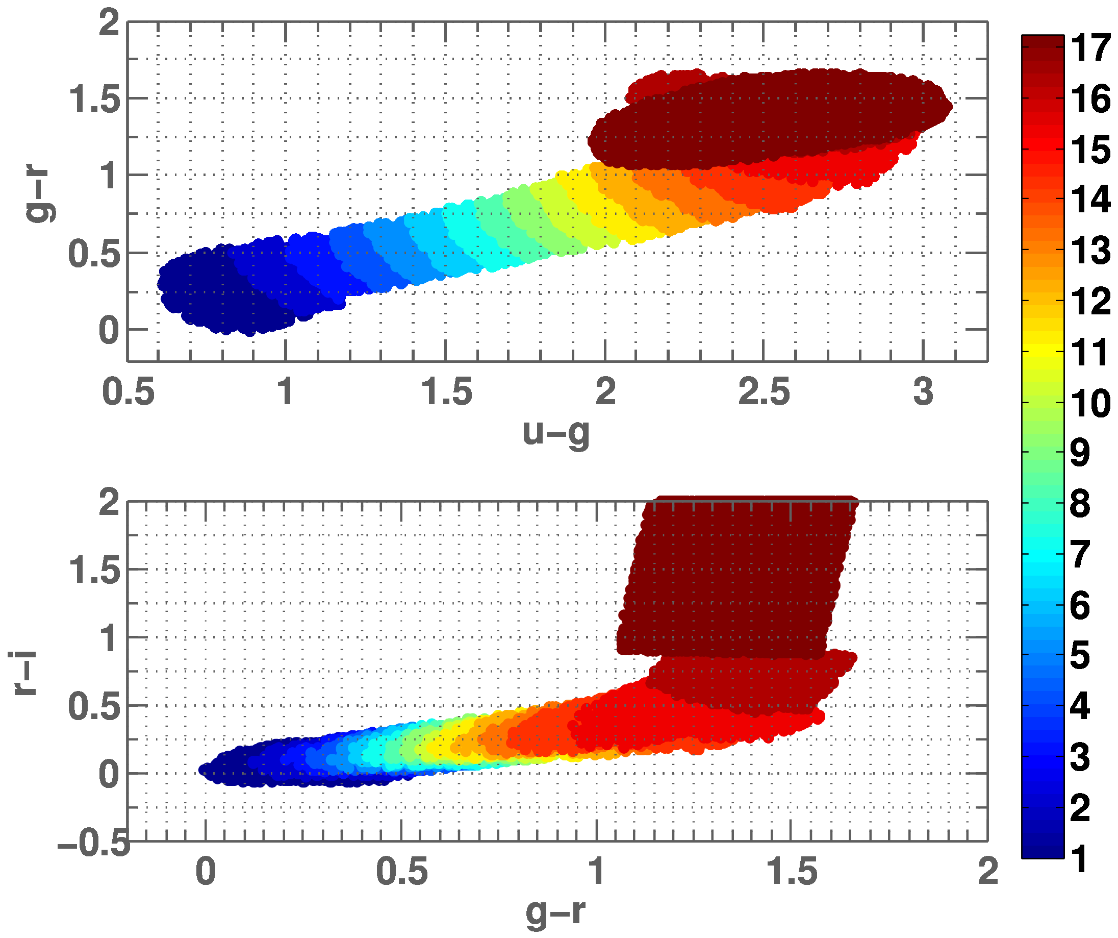
Figure 13: The $g-r$ versus $u-g$ and $r-i$ versus $g-r$ colour–colour planes of the stellar locus in our emulation of the “low-z” (i.e. $ugri$) SDSS quasar selection criteria Richards et al. (2002). This figure is very similar to their figures 2 & 3. The colour of a plotted point encodes the number of the nearest “stellar locus point”, as defined in table 3 of Richards et al. (2002). The plotted points define the projection of the 4-$\sigma$ error surface and were determined by Monte Carlo sampling. Objects with zero photometric errors will be selected as quasar candidates if they fall outside this surface. We note that, although our stellar loci plots are very similar to those ones of Richards et al. (2002), there are some small differences that we can not account for, so users of our code should test it specifically for their purposes to ensure reliable statistical results.

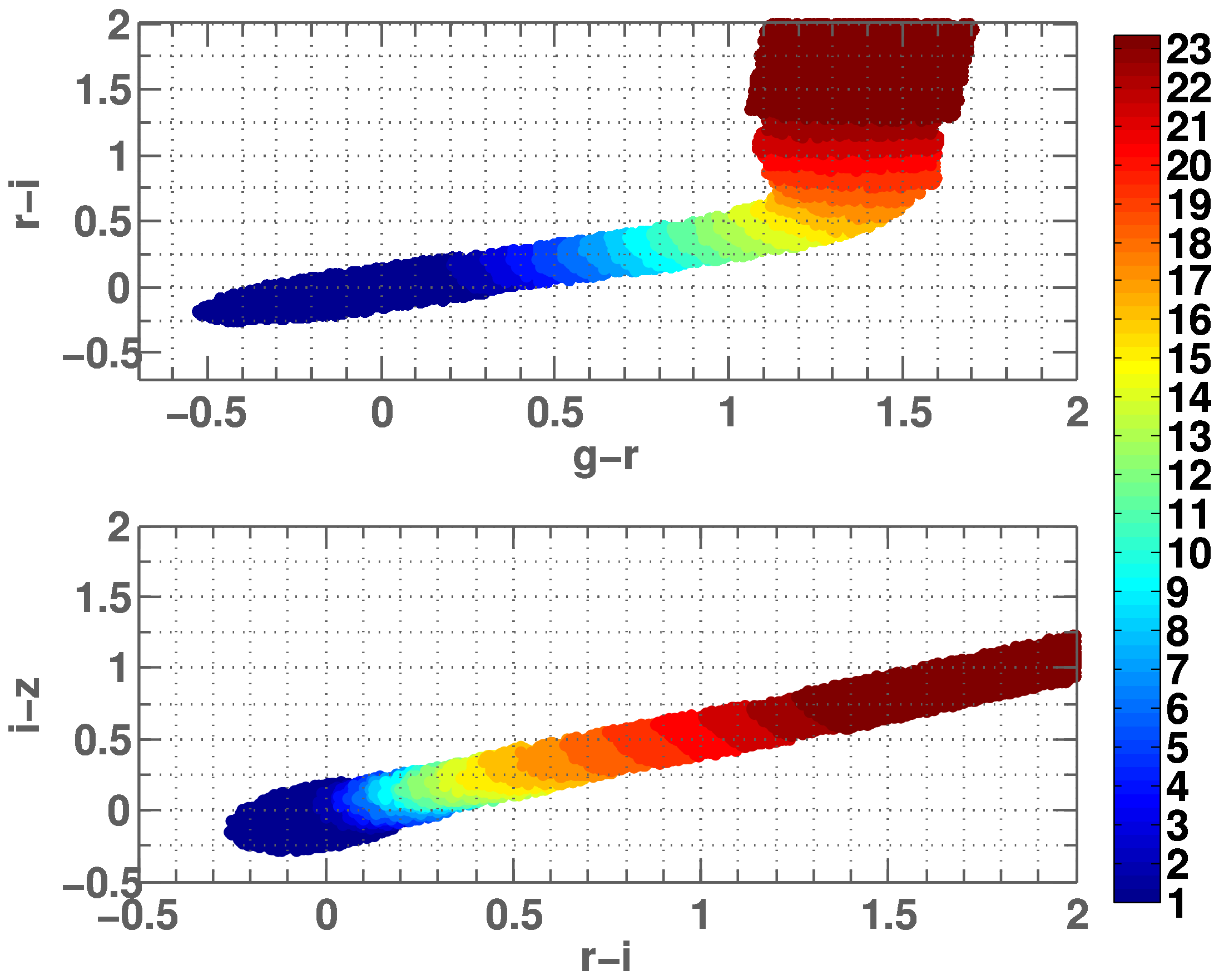
Figure 14: Same as Figure 14 but for the $r-i$ versus $g-r$ and $i-z$ versus $r-i$ colour–colour plane for the “high-z” (i.e. $griz$) quasar selection criteria. This figure is very similar to figures 5 & 6 of Richards et al. (2002) and the colour of a plotted point encodes the number of the nearest “stellar locus point” defined their table 4.

A further, simple test of our code is to check whether it selects quasar candidates via the same selection channel as specified by Schneider et al. (2010). For this test we use the entire sample of $2.2<z_{\textrm{\scriptsize em}}<4.42$ quasars in the Noterdaeme et al. (2009b) catalogue from which our reddening analysis stems. Inputting the target PSF photometry of these quasars into our code results in 60 per cent of them being selected via the $ugri$ channel and 62 per cent via the $griz$ channel (noting that each object can be selected by either, both or neither channel). These values are similar to, though slightly higher than, the values of 51 and 59 per cent, as defined by the classification of Schneider et al. (2010) using the same selection algorithm as in Richards et al. (2002). Again, although these differences are not important for assessing the degree of bias entering our dust-reddening analysis (especially in light of the results in Figure 10), it is possible that such differences are important for other high-precision, statistical studies with large samples, so we again recommend further, specific reliability tests in those circumstances.

Supporting Information

Additional Supporting Information may be found in the online version of this article:

Table 1. The DLA quasar sample (774 quasars).
Table 2. The absorber quasar sample (1069 quasars).
Table 3. The non-DLA quasar sample (7105 quasars).
Table 4. The non-absorber quasar sample (6733 quasars).

Please note: Oxford University Press are not responsible for the content or functionality of any supporting materials supplied by the authors. Any queries (other than missing material) should be directed to the corresponding author for the paper.

References

- Akerman et al. (2005) Akerman C. J., Ellison S. L., Pettini M., Steidel C. C., 2005, A&A, 440, 499
- Aller et al. (2012) Aller M. C., Kulkarni V. P., York D. G., Vladilo G., Welty D. E., Som D., 2012, ApJ, 748, 19
- Aller et al. (2014) Aller M. C., Kulkarni V. P., York D. G., Welty D. E., Vladilo G., Liger N., 2014, ApJ, 785, 36
- Asplund et al. (2009) Asplund M., Grevesse N., Sauval A. J., Scott P., 2009, ARA&A, 47, 481
- Becker et al. (1995) Becker R. H., White R. L., Helfand D. J., 1995, ApJ, 450, 559
- Bernet & Murphy (2015) Bernet M. L., Murphy M. T., 2015, SDSS_QSOsel_Bernet: First release, doi:10.5281/zenodo.31470
- Cardelli et al. (1989) Cardelli J. A., Clayton G. C., Mathis J. S., 1989, ApJ, 345, 245
- Crighton et al. (2015) Crighton N. H. M. et al., 2015, MNRAS, 452, 217
- Draine (2003) Draine B. T., 2003, ARA&A, 41, 241
- Ellison et al. (2001) Ellison S. L., Yan L., Hook I. M., Pettini M., Wall J. V., Shaver P., 2001, A&A, 379, 393
- Ellison et al. (2005) Ellison S. L., Hall P. B., Lira P., 2005, AJ, 130, 1345
- Fall & Pei (1989) Fall S. M., Pei Y. C., 1989, ApJ, 337, 7
- Fall & Pei (1993) Fall S. M., Pei Y. C., 1993, ApJ, 402, 479
- Fall et al. (1989) Fall S. M., Pei Y. C., McMahon R. G., 1989, ApJ, 341, L5
- Fitzpatrick (1985) Fitzpatrick E. L., 1985, ApJ, 299, 219
- Frank & Péroux (2010) Frank S., Péroux C., 2010, MNRAS, 406, 2235
- Fukugita & Ménard (2015) Fukugita M., Ménard B., 2015, ApJ, 799, 195
- Jenkins (1987) Jenkins E. B., 1987, in Hollenbach D. J., Thronson Jr. H. A., eds, Astrophys. Space Sci. Libr. Vol. 134, Interstellar Processes. pp 533–559
- Jenkins & Peimbert (1997) Jenkins E. B., Peimbert A., 1997, ApJ, 477, 265
- Jiang et al. (2010) Jiang P., Ge J., Prochaska J. X., Wang J., Zhou H., Wang T., 2010, ApJ, 724, 1325
- Jorgenson et al. (2006) Jorgenson R. A., Wolfe A. M., Prochaska J. X., Lu L., Howk J. C., Cooke J., Gawiser E., Gelino D. M., 2006, ApJ, 646, 730
- Jorgenson et al. (2013) Jorgenson R. A., Murphy M. T., Thompson R., 2013, MNRAS, 435, 482
- Jorgenson et al. (2014) Jorgenson R. A., Murphy M. T., Thompson R., Carswell R. F., 2014, MNRAS, 443, 2783
- Junkkarinen et al. (2004) Junkkarinen V. T., Cohen R. D., Beaver E. A., Burbidge E. M., Lyons R. W., Madejski G., 2004, ApJ, 614, 658
- Kaplan et al. (2010) Kaplan K. F., Prochaska J. X., Herbert-Fort S., Ellison S. L., Dessauges-Zavadsky M., 2010, PASP, 122, 619
- Khare et al. (2007) Khare P., Kulkarni V. P., Péroux C., York D. G., Lauroesch J. T., Meiring J. D., 2007, A&A, 464, 487
- Khare et al. (2012) Khare P., Vanden Berk D., York D. G., Lundgren B., Kulkarni V. P., 2012, MNRAS, 419, 1028
- Kulkarni et al. (2007) Kulkarni V. P., York D. G., Vladilo G., Welty D. E., 2007, ApJ, 663, L81
- Kulkarni et al. (2011) Kulkarni V. P., Torres-Garcia L. M., Som D., York D. G., Welty D. E., Vladilo G., 2011, ApJ, 726, 14
- Kurt & Dufour (1998) Kurt C. M., Dufour R. J., 1998, in Dufour R. J., Torres-Peimbert S., eds, Revista Mexicana de Astron. Astrofisica Conf. Series Vol. 7, The sixth Texas–Mexico conference on astrophysics: astrophysical plasmas – near and far. p. 202
- Lanzetta et al. (1995) Lanzetta K. M., Wolfe A. M., Turnshek D. A., 1995, ApJ, 440, 435
- Ledoux et al. (2002) Ledoux C., Bergeron J., Petitjean P., 2002, A&A, 385, 802
- Ledoux et al. (2003) Ledoux C., Petitjean P., Srianand R., 2003, MNRAS, 346, 209
- Ma et al. (2015) Ma J. et al., 2015, MNRAS, 454, 1751
- Martin et al. (1989) Martin N., Maurice E., Lequeux J., 1989, A&A, 215, 219
- Murphy & Liske (2004) Murphy M. T., Liske J., 2004, MNRAS, 354, L31
- Neeleman et al. (2013) Neeleman M., Wolfe A. M., Prochaska J. X., Rafelski M., 2013, ApJ, 769, 54
- Newberg & Yanny (1997) Newberg H. J., Yanny B., 1997, ApJS, 113, 89
- Noterdaeme et al. (2009a) Noterdaeme P., Ledoux C., Srianand R., Petitjean P., Lopez S., 2009a, A&A, 503, 765
- Noterdaeme et al. (2009b) Noterdaeme P., Petitjean P., Ledoux C., Srianand R., 2009b, A&A, 505, 1087
- O’Donnell (1994) O’Donnell J. E., 1994, ApJ, 422, 158
- Ostriker & Heisler (1984) Ostriker J. P., Heisler J., 1984, ApJ, 278, 1
- Pâris et al. (2012) Pâris I. et al., 2012, A&A, 548, 66
- Pâris et al. (2014) Pâris I. et al., 2014, A&A, 563, A54
- Pei (1992) Pei Y. C., 1992, ApJ, 395, 130
- Pei et al. (1991) Pei Y. C., Fall S. M., Bechtold J., 1991, ApJ, 378, 6
- Pettini et al. (1997) Pettini M., King D. L., Smith L. J., Hunstead R. W., 1997, ApJ, 478, 536
- Pontzen & Pettini (2009) Pontzen A., Pettini M., 2009, MNRAS, 393, 557
- Prochaska & Wolfe (2009) Prochaska J. X., Wolfe A. M., 2009, ApJ, 696, 1543
- Prochaska et al. (2005) Prochaska J. X., Herbert-Fort S., Wolfe A. M., 2005, ApJ, 635, 123
- Prochaska et al. (2008) Prochaska J. X., Chen H.-W., Wolfe A. M., Dessauges-Zavadsky M., Bloom J. S., 2008, ApJ, 672, 59
- Rafelski et al. (2012) Rafelski M., Wolfe A. M., Prochaska J. X., Neeleman M., Mendez A. J., 2012, ApJ, 755, 89
- Reichard et al. (2003) Reichard T. A. et al., 2003, AJ, 125, 1711
- Richards et al. (2002) Richards G. T. et al., 2002, AJ, 123, 2945
- Schlegel et al. (1998) Schlegel D. J., Finkbeiner D. P., Davis M., 1998, ApJ, 500, 525
- Schneider et al. (2007) Schneider D. P. et al., 2007, AJ, 134, 102
- Schneider et al. (2010) Schneider D. P. et al., 2010, AJ, 139, 2360
- Shen et al. (2011) Shen Y. et al., 2011, ApJS, 194, 45
- Vanden Berk et al. (2001) Vanden Berk D. E. et al., 2001, AJ, 122, 549
- Viegas (1995) Viegas S. M., 1995, MNRAS, 276, 268
- Vladilo (2002) Vladilo G., 2002, ApJ, 569, 295
- Vladilo & Péroux (2005) Vladilo G., Péroux C., 2005, A&A, 444, 461
- Vladilo et al. (2008) Vladilo G., Prochaska J. X., Wolfe A. M., 2008, A&A, 478, 701
- Wang et al. (2004) Wang J., Hall P. B., Ge J., Li A., Schneider D. P., 2004, ApJ, 609, 589
- Wang et al. (2012) Wang J.-G. et al., 2012, ApJ, 760, 42
- Wolfe (1986) Wolfe A. M., 1986, R. Soc. London Philos. Trans. Series A, 320, 503
- Wolfe et al. (1986) Wolfe A. M., Turnshek D. A., Smith H. E., Cohen R. D., 1986, ApJS, 61, 249
- Wolfe et al. (2003a) Wolfe A. M., Prochaska J. X., Gawiser E., 2003a, ApJ, 593, 215
- Wolfe et al. (2003b) Wolfe A. M., Gawiser E., Prochaska J. X., 2003b, ApJ, 593, 235
- Wolfe et al. (2005) Wolfe A. M., Gawiser E., Prochaska J. X., 2005, ARA&A, 43, 861
- Zhou et al. (2010) Zhou H., Ge J., Lu H., Wang T., Yuan W., Jiang P., Shan H., 2010, ApJ, 708, 742