Evidence for the Thermal Sunyaev-Zel’dovich Effect Associated with Quasar Feedback

Abstract

Using a radio-quiet subsample of the Sloan Digital Sky Survey spectroscopic quasar catalogue, spanning redshifts 0.5–3.5, we derive the mean millimetre and far-infrared quasar spectral energy distributions (SEDs) via a stacking analysis of Atacama Cosmology Telescope and Herschel-Spectral and Photometric Imaging REceiver data. We constrain the form of the far-infrared emission and find 3$\sigma$–4$\sigma$ evidence for the thermal Sunyaev-Zel’dovich (SZ) effect, characteristic of a hot ionized gas component with thermal energy $(6.2\pm 1.7)~{}\times~{}10^{60}$ erg. This amount of thermal energy is greater than expected assuming only hot gas in virial equilibrium with the dark matter haloes of $(1-5)\times~{}10^{12}h^{-1}$M_⊙ that these systems are expected to occupy, though the highest quasar mass estimates found in the literature could explain a large fraction of this energy. Our measurements are consistent with quasars depositing up to $(14.5\pm 3.3)~{}\tau_{8}^{-1}$ per cent of their radiative energy into their circumgalactic environment if their typical period of quasar activity is $\tau_{8}\times~{}10^{8}$ yr. For high quasar host masses, $\sim 10^{13}h^{-1}$M_⊙, this percentage will be reduced. Furthermore, the uncertainty on this percentage is only statistical and additional systematic uncertainties enter at the 40 per cent level. The SEDs are dust dominated in all bands and we consider various models for dust emission. While sufficiently complex dust models can obviate the SZ effect, the SZ interpretation remains favoured at the 3$\sigma$–4$\sigma$ level for most models.

1 Introduction

Feedback from accreting black holes has become a key element in modelling galaxy evolution (Tabor & Binney, 1993; Silk & Rees, 1998; Springel et al., 2005). Quasar feedback is routinely invoked in galaxy formation models to quench star formation and to explain the steep decline of the bright end of the luminosity function of galaxies (Thoul & Weinberg, 1995; Croton et al., 2006) and to reheat the intracluster medium (e.g., Rawlings & Jarvis, 2004; Scannapieco & Oh, 2004). The discovery that the masses of supermassive black holes in inactive galaxies strongly correlate with the velocity dispersions and masses of their hosts’ stellar bulges (Magorrian et al., 1998; Gebhardt et al., 2000; Ferrarese & Merritt, 2000) also suggests that the energy output of the black hole in its quasar phase must be somehow coupled to the gas from which the stars form (Hopkins et al., 2006). Finally, the similarity of the history of star formation activity and that of supermassive black hole accretion in the Universe (Boyle & Terlevich, 1998; Hopkins et al., 2008) suggests that these two phenomena physically affect each other or result from the same physical process. Both star formation activity and black hole accretion activity peak at $z>2$ and rapidly decline afterward; thus it is at these high redshifts that the physical connection between supermassive black holes and their hosts was established.

How can supermassive black holes so profoundly affect their large-scale galactic and even intergalactic environments? Even a small fraction of the binding energy of material accreted by the supermassive black hole is in principle sufficient to liberate the galaxy-scale gas from the galaxy potential, but coupling this energy output to the surrounding gas is no trivial task. However, there are circumstances in which accretion energy clearly has had an impact on its environment. Radio jets in massive elliptical galaxies and brightest cluster galaxies deposit energy into the hot gas envelope (McNamara & Nulsen, 2007; Fabian, 2012). Likewise, powerful radio jets entrain warm gas and carry significant amounts of material out of their host galaxies, especially at high redshifts (van Breugel et al., 1986; Tadhunter, 1991; Villar-Martín et al., 1999; Nesvadba et al., 2006, 2008; Fu & Stockton, 2009). While a narrow collimated outflow might seem inefficient at impacting and removing the surrounding matter, in practice the power of the jet is quickly and efficiently thermalized if it propagates into high density material (Begelman & Cioffi, 1989).

Radio-quiet quasars (those that do not seem to have powerful radio jets) can also have a strong effect on their large-scale environment. Radiation pressure, especially through absorption in bound-bound transitions (Murray et al., 1995; Proga et al., 2000), can accelerate material in the immediate vicinity of the black hole ($\la 1000$ Schwarzschild radii) to velocities $\la 10\%$ of the speed of light. This material then impacts the interstellar medium in the host galaxy (Faucher-Giguère & Quataert, 2012; Zubovas & King, 2012; Nims et al., 2015), drives shocks into the surrounding medium, accelerates and destroys high-density clouds (Mac Low et al., 1994), and over the lifetime of the quasar the resulting wind can engulf the entire galaxy. High-velocity outflows on nuclear scales are observed in a large fraction of all quasars (Weymann et al., 1981; Turnshek, 1984; Crenshaw et al., 2003; Reichard et al., 2003; Gallagher et al., 2007), but evidence for large-scale impact of these outflows has long been elusive. Only the last few years have brought about a flood of observations of powerful, galaxy-wide outflows launched by radio-quiet quasars (Arav et al., 2008; Moe et al., 2009; Alexander et al., 2010; Greene et al., 2011; Cano-Díaz et al., 2012; Liu et al., 2013a, b; Hainline et al., 2013; Rupke & Veilleux, 2013; Veilleux et al., 2013; Harrison et al., 2014; Hainline et al., 2014; Zakamska & Greene, 2014; Brusa et al., 2015a; Carniani et al., 2015; Harrison et al., 2015; Perna et al., 2015; Brusa et al., 2015b).

Quasar-driven winds are likely to be inhomogeneous, with different phases of the wind medium observable in different domains of the electromagnetic spectrum. The simplest models for these winds involve hot, low density, volume-filling plasma (Faucher-Giguère & Quataert, 2012; Zubovas & King, 2012), with higher density clumps, shells or filaments. The warmer of those ($T\simeq 10^{4}$K) produce optical emission lines, and cooler (and denser) clumps may exist in neutral or even molecular form. Thus, the physical conditions in quasar-driven winds are qualitatively similar to those in starburst-driven winds, where the different phases are directly observable and spatially resolved in some nearby galaxies (Heckman et al., 1990; Veilleux et al., 1994). It is at present not known which of the phases of the quasar winds carries most of the mass, momentum and energy; obtaining these measurements is critical for understanding the full impact of quasars on galaxy formation.

The hot volume-filling component is particularly elusive because of its extremely low density, which implies that any emission associated with it would be very weak (Greene et al., 2014). The Sunyaev-Zeldovich (SZ) effect (Sunyaev & Zeldovich, 1970) offers a unique opportunity to detect and characterize the bulk of quasar-driven winds. The SZ effect manifests itself as a spectral distortion of the cosmic microwave background (CMB) that occurs when CMB photons inverse-Compton scatter off intervening hot ionized gas. Most importantly, the magnitude of the total integrated SZ effect is proportional to the total thermal energy of the hot ionized gas and thus allows us to measure the thermalized energetic output from the AGN, which is not detectable by other methods. Furthermore, the surface brightness of the SZ effect is not subject to dimming with redshift, facilitating the study of high-$z$ systems of low-density with ionized gas that is too faint to be studied in emission with current facilities.

Fortunately, measurements of the SZ effect have recently reached a maturity that enables investigations of AGN feedback. Although the SZ effect was theorized over 40 years ago as a CMB spectral distortion by hot gas around galaxy clusters, only within the past 5 years have measurements of the SZ effect begun to reach their potential with detections of hundreds of clusters in millimetre-wave surveys by the Atacama Cosmology Telescope (ACT), the South Pole Telescope (SPT) and the Planck satellite (Hasselfield et al., 2013a; Bleem et al., 2015; Planck Collaboration et al., 2015). The SZ effect associated with the ionized circumgalactic medium of individual galaxies or galaxy groups is generally too weak to be directly detected in these surveys. However, the large area of these surveys has enabled measurements of the average SZ effect associated with ensembles of these lower mass systems selected from overlapping optical surveys (Hand et al., 2011; Planck Collaboration et al., 2013; Greco et al., 2015; Spacek et al., 2016). These measurements and associated hydrodynamic simulations (Battaglia et al., 2012; Le Brun et al., 2015) consider the effects of AGN feedback processes on the mean gas distribution and the scaling of the SZ effect with halo mass. The aforementioned studies, however, do not distinguish systems with ongoing AGN feedback from those without, focusing instead on the bulk sample with mass as the defining independent variable.

The SZ effect in systems with ongoing feedback has been forecast through both analytic estimates (Yamada et al., 1999; Natarajan & Sigurdsson, 1999; Platania et al., 2002; Pfrommer et al., 2005; Chatterjee & Kosowsky, 2007) and simulations (Chatterjee et al., 2008; Scannapieco et al., 2008; Prokhorov et al., 2010, 2012; Cen & Safarzadeh, 2015b). As discussed above, however, key details of the energy transfer mechanism (and therefore the source of the SZ effect) are not known and will depend on the characteristics of the system (e.g., radio-loud versus radio-quiet). Therefore measurements are essential for progress. Given the angular resolution and sensitivity of present millimetre-wave surveys, these measurements are limited to integrated measurements of the SZ effect over the entire volume of the circumgalactic medium. With this single integrated measurement, the SZ effect due to AGN feedback will only be distinguishable from an active system’s in situ SZ effect from gravitational heating (virialization) if the feedback significantly alters the internal thermal energy of the system during the active phase. For radio-loud AGN, Gralla et al. (2014) found that the internal thermal energy due to virial equilibrium could explain the observed SZ effect, implying that energy from AGN feedback did not significantly alter the total thermal energy. The average halo mass of radio-loud AGN ($\gtrsim 10^{13}h^{-1}$ M_⊙) is found to be an order of magnitude greater than that of radio-quiet quasars in optical lensing studies at redshifts $z<0.3$ (Mandelbaum et al., 2009). Thus the SZ effect from virialized gas associated with radio-quiet quasars at these redshifts should be one to two orders of magnitude less than that of their radio-loud counterparts. Therefore, one may hope to distinguish the SZ effect due to feedback in these lower mass systems from that due to virial equilibrium. However, the characteristic mass of quasars at high redshift is less constrained, with estimates in the range $(1-5)\times 10^{12}h^{-1}$M_⊙ (White et al., 2012; Shen et al., 2013; Wang et al., 2015) and up to $10^{13}h^{-1}$ M_⊙ (Richardson et al., 2012). Progress towards understanding feedback in these high-$z$ quasars is therefore limited by these uncertainties on their mass.

Initial studies of the SZ-effect in quasars from the Sloan Digital Sky Survey (SDSS) have used data from the Wilkinson Microwave Anisotropy Probe (Chatterjee et al., 2010) and the Planck satellite (Ruan et al., 2015). In these studies, in Gralla et al. (2014), and in this work, a major challenge is estimating the SZ effect in the presence of emission from the AGN and its host. In radio-selected systems, as used in Gralla et al. (2014), and at lower frequencies, as used in Chatterjee et al. (2010), the synchrotron emission from electrons accelerated by the AGN must be modelled. At higher frequencies dust becomes an important factor for all quasar hosts, but especially those with substantial ongoing star formation rates. (Radio-selected systems live primarily in massive elliptical systems with lower rates.) Different approaches, including spectral energy distribution (SED) modelling (Chatterjee et al., 2010; Gralla et al., 2014) and internal linear combination methods (Ruan et al., 2015), have been used to disentangle the SZ effect from the emission component. This study uses SED modelling as in Gralla et al. (2014) but with the important advantage of having redshift measurements for all the systems. We will return to consider the previous studies and energetics as measured by the SZ effect in the discussion of our results.

In this paper, we statistically search for the hot haloes around quasars with the SZ effect in a large sample of radio-quiet quasars from the SDSS (York et al., 2000; Schneider et al., 2010; Eisenstein et al., 2011; Pâris et al., 2014) using millimetre/submillimetre data from the ACT and Herschel-SPIRE. We describe the data in Section 2 and our stacking analysis in Section 3. We discuss our modelling technique and its results in Section 4 and the implications of these results in Section 5. We conclude in Section 6. Unless specified otherwise, we assume a flat $\Lambda$ cold dark matter cosmology with $\Omega_{\rm M}=0.30$ and $\Omega_{\Lambda}=0.70$. The Hubble constant is parametrized as $H_{0}=70h_{70}$ km s^-1 Mpc^-1 and if no factor is stated $h_{70}=1$ has been used. For halo mass values quoted from the literature, we use the conventional unit of $h^{-1}{\rm M}_{\odot}$ where $h=H_{0}/(100$ km s^-1 Mpc^-1). The function $E(z)=\sqrt{\Omega_{\rm M}(1+z)^{3}+\Omega_{\Lambda}}$ describes the evolution of the Hubble parameter, $H(z)=H_{0}E(z)$.

2 Data

2.1 ACT Data

ACT is a six-metre survey telescope for millimetre-wave astronomy operating in the Atacama Desert high in the Andes of northern Chile (Fowler et al., 2007; Swetz et al., 2011). Since 2007, ACT has surveyed more than 1000 square degrees of sky at declinations both south of and on the celestial equator. The reduction, calibration and beam determination for the ACT data are described in Dünner et al. (2013), Hajian et al. (2011), and Hasselfield et al. (2013b). During the years 2007–2010, ACT was equipped with the Millimetre Bolometric Array Camera (MBAC), which operated at 148, 218, and 277 GHz, frequencies well suited for studying the CMB, the SZ effect, and thermal dust emission. In 2013, ACT was equipped with a new polarization-sensitive receiver and became ACTPol with a revised frequency coverage focused on 90 and 150 GHz (Niemack et al., 2010). The data used in this study derive from the original ACT observations obtained on the celestial equator from 2008 to 2010. This three frequency (148, 218, and 277 GHz) data set is the same as used in the study of millimetre emission and the SZ effect in radio-loud AGN of Gralla et al. (2014). The survey area is approximately 340 square degrees ($-55\degr\leq\alpha\leq 58\degr$, $-1\aas@@fstack{\circ}5\leq\delta\leq 1\aas@@fstack{\circ}5$). In Table 1 we summarize the properties of the ACT data. The instrument beams were measured using Saturn (Hasselfield et al., 2013b). The 148 GHz data were calibrated through cross-correlation with WMAP (Hajian et al., 2011). The 148 GHz calibration was transferred through cross-correlation to the 218 GHz data. As a result, the uncertainties in flux calibration of the 148 and 218 GHz data are correlated at the level of 60%. The 277 GHz data are calibrated from Uranus (Hasselfield et al., 2013b). Flux densities were estimated from a matched filtered map as described in Marsden et al. (2014). The flux calibration uncertainties in Table 1 include conservative estimates of error due to uncertainty in beam solid angle, absolute calibration and map-making flux density recovery. We refer the reader to Gralla et al. (2014) for more details. ACT is well suited to this study due to its frequency coverage, which spans the SZ spectrum, and its small beam size. ACT’s arcminute scale resolution provides an advantage in sensitivity to the stacked quasar signal (over e.g. WMAP and Planck) while maintaining a large survey area allowing for sufficient overlap with existing surveys and catalogues.

2.2 Herschel-SPIRE Data

The Herschel Space Observatory Spectral and Photometric Imaging REceiver (SPIRE) observed at frequencies of 600, 857 and 1200 GHz (Griffin et al., 2010). For this study we use the publicly available Herschel Stripe 82 Survey (HerS; Viero et al., 2014). HerS covers 79 square degrees overlapping the celestial equator ($13\degr<\alpha<37\degr$, $-2\degr<\alpha<2\degr$). The properties of HerS are listed in Table 1. The SPIRE flux calibration uncertainty and beam full width at half-maximum (FWHM) are derived from observations of Neptune (Griffin et al., 2013). A significant fraction of the typical rms noise values for Herschel-SPIRE flux recovery, as quoted in Table 1, originates from confusion noise of the order of 8 mJy beam^-1 (Viero et al., 2014).

Table 1: ACT and HerS survey parameters.

	ACT			HerS
Band	148 GHz	218 GHz	277 GHz	600 GHz	857 GHz	1200 GHz
Beam FWHM	1.4 arcmin	1.0 arcmin	0.9 arcmin	0.6 arcmin	0.4 arcmin	0.3 arcmin
Typical rms noise (mJy beam-1)	2.2	3.3	6.5	13.3	12.9	14.8
Flux calibration uncertainty (per cent)	3$a$	5$a$	15	7$b$	7$b$	7$b$

• A correlated component to the calibration uncertainty of 3 per cent between the ACT 148 and 218 GHz bands is also accounted for.

• The calibration uncertainty of the Herschel-SPIRE data includes a 5 per cent component correlated across all three bands.

2.3 SDSS Quasar Catalogue

For this study we use the SDSS optical quasar catalogues derived from the spectroscopic quasar samples in Data Release 7 (DR7; Schneider et al., 2010) and Data Release 10 (DR10; Pâris et al., 2014). We select all quasars within the ACT equatorial survey. Any object present in both DR7 and DR10 is included only once. This combined catalogue spans a wide range of redshift out to $z\sim 7$. As we will be performing a statistical analysis on this sample, we cut the catalogue to lie within the well populated redshift range $0.5<z<3.5$, where 95% of the quasars are found. Due to the statistical nature of this work, the primary benefit of using a spectroscopic catalogue is not the redshift precision it provides but the robust identification of objects as quasars which the SDSS spectroscopic classification pipeline enables. We additionally cut this catalogue by excising all quasars that lie within $2.5$ arcmin of sources detected with significance $>5\sigma$ in the ACT millimetre data. Detected ACT sources are typically extremely luminous blazars, local ($z\ll 1$) star-forming galaxies, or high-$z$ lensed dusty star-forming galaxies (Marsden et al., 2014). Due to their high millimetre fluxes and the manner in which the ACT maps are filtered, these objects may significantly contaminate the measured fluxes of nearby quasars. However, we find that neglecting this cut alters the stacked fluxes (see Section 3) by no more than $1\sigma$, and extending the mask to 5 arcmin around detected sources produces a change in the stacked signal much smaller than the statistical uncertainties on these data.

ACT galaxy clusters detected through the SZ effect are typically found at moderate significance and, with redshifts $z\lesssim 1$, should not be strongly correlated with the quasar catalogue or contaminate our results. We therefore do not excise these objects. The catalogue obtained after these cuts contains 17468 quasars (8642 from DR7 and 8826 from DR10). A subset of 3833 of these objects additionally overlap with the HerS region. Fig. 1 shows the redshift distribution of this quasar sample as well as the redshift distribution of those quasars that additionally overlap with the Herschel-SPIRE HerS region. The sharp increase in sources at $z>2$ shown in Fig. 1 is due to the BOSS selection in DR10. The non-uniformity of this sample’s selection is mitigated in our results by binning in redshift as described in Section 3. We additionally construct estimates for the optical bolometric luminosity of each quasar in the sample by applying the bolometric correction from Richards et al. (2006a) as described in Appendix A.

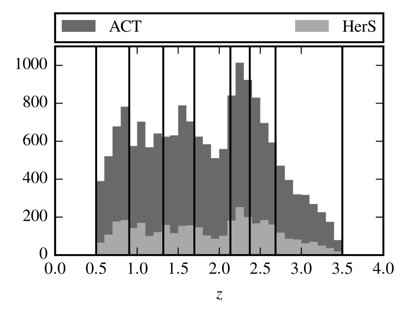
Figure 1: The redshift distribution of the combined SDSS DR7 and DR10 spectroscopic quasar sample falling within the ACT equatorial region ($-55\degr\leq\alpha\leq 58\degr$, $-1\aas@@fstack{\circ}5\leq\delta\leq 1\aas@@fstack{\circ}5$) after the radio loud cut has been applied. The histogram of the entirety of this sample is shown in dark grey and the subset which lies within the HerS region is shown in light grey. The vertical black lines denote the boundaries of the redshift bins we use for the stacking analysis.

2.4 Radio Loud Cut

Since we are interested in detecting the SZ effect, which is most prominent at millimetre wavelengths, we further cut this catalogue to exclude potentially radio-loud quasars. This acts to minimize contamination of the SZ signal from synchrotron emission. We perform a radio-quiet classification based on the methods of Xu et al. (1999). This study finds a bimodal distribution in the ratio of AGN radio luminosity at 5 GHz and [OIII] 5007 Å line luminosity (an orientation insensitive measure of the AGN intrinsic luminosity) and defines a cut based on this bimodality. We use the mean relation given in Reyes et al. (2008) between $\mathcal{M}_{2500}$, the absolute magnitude at the rest-frame wavelength of 2500 Å, and $L_{\rm[OIII]}$. Here, as in Reyes et al. (2008), we use the SDSS $i$ band absolute magnitude $\mathcal{M}_{I}(z=2)$ (Richards et al., 2006b) as a proxy for $\mathcal{M}_{2500}$, which is valid for $z\sim 2$. To determine the radio luminosities, we use the matched 1.4 GHz fluxes obtained from the Faint Images of the Radio Sky at Twenty-cm (FIRST; Becker et al., 1995) survey that are included in the DR7 and DR10 quasar catalogues. These 1.4 GHz radio fluxes are related to $L_{\rm 5GHz}$ using the catalogue redshifts and assuming a synchrotron spectrum, $L_{\nu}\propto\nu^{-1}$. This radio-loud cut shifts the stacked fluxes (as described in Section 3) in the 148 and 218 GHz bands by at most 1$\sigma$ in any redshift bin and reduces the sample size by 412 (2%). This cut removes the majority of sources that are detected by the FIRST survey. Applying stricter cuts on the radio luminosities has a negligible effect on our results.

3 Stacking Analysis

The typical submillimetre flux densities of optically selected quasars are found to be significantly less than the detection limits of the ACT and Herschel-SPIRE data. We therefore employ a stacking analysis to measure the ensemble flux densities associated with the quasars. Stacking can be shown to be an unbiased maximum likelihood estimator of the mean flux density of a catalogue in both the case of a Gaussian noise background, as is the case for the point source-filtered ACT data, or for the confusion-limited Herschel-SPIRE data (Marsden et al., 2009; Viero et al., 2013).

Due to both the non-uniform selection of our sample in redshift and the strong redshift dependence of our estimated bolometric luminosities (See Figs 1 and 5) we choose to bin the quasar catalogue by redshift prior to stacking. This additionally allows us to account for the redshift dependence of the parameters of the models to be fit. We choose these bins such that they each contain approximately equal numbers of sources. For the seven redshift bins thus chosen, we have approximately 2430 quasars per bin. The boundaries of these bins are shown as the vertical lines in Figs. 1 and 5. As the catalogue was selected to lie within the ACT equatorial region all of these objects contribute to the stacks for the 148, 218 and 277 GHz bands. For the 600, 857 and 1200 GHz Herschel-SPIRE bands the number of quasars that contribute is further diminished by the band dependent masks which account for varying sky coverage of the data. The smaller sky coverage of the HeRS survey results in 506–574 quasars per bin with submillimetre data.

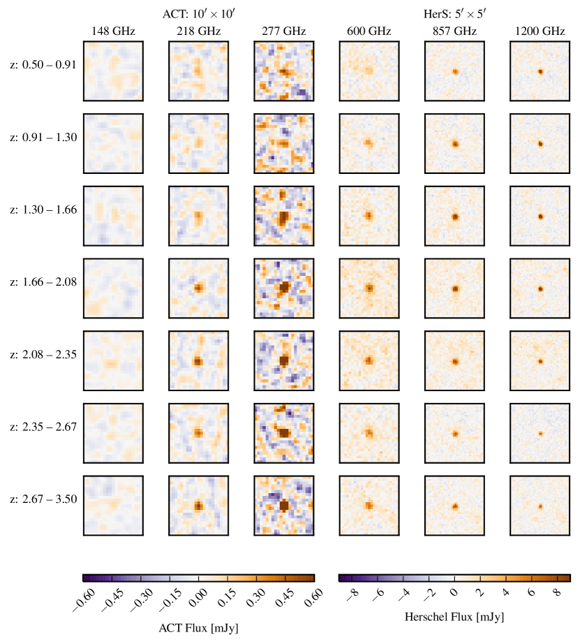
Figure 2: Weighted average thumbnail images around the quasar positions in 10 arcmin $\times$ 10 arcmin stamps for the matched filtered ACT data (left three columns) and 5 arcmin $\times$ 5 arcmin stamps for the Herschel-SPIRE data (right three columns). The observed signal is dominated by the dust emission associated with quasars. Since no background aperture has been subtracted from the Herschel-SPIRE data here, large scale excess positive signal, associated with correlated cosmic infrared background emission, is visible.

For each of the redshift bins, we construct the stacked signal in a band by taking the inverse variance weighted average of the measured flux density corresponding to each source in the bin:

$$\bar{d}_{\nu}^{\alpha}=\frac{\sum_{i}^{N^{\alpha}}w_{i,\nu}d_{i,\nu}}{\sum_{i}^{N^{\alpha}}w_{i,\nu}}.$$ (1)

This yields the stacked signal $\bar{d}_{\nu}^{\alpha}$ of the redshift bin $\alpha$ containing $N^{\alpha}$ sources, each contributing flux density $d_{i,\nu}$ in the band corresponding to a frequency $\nu$. The inverse variance weights $w_{i,\nu}$, which vary from source to source and between bands, are determined from the error maps for each data set. For the Herschel-SPIRE data, these error maps are derived from the diagonal component of the pixel-pixel covariance matrices that are a product of the map making pipeline (Patanchon et al., 2008). For the matched filtered ACT data, we take the variance in a pixel for a given band to be inversely proportional to the value of that band’s hits-count map at that location. The flux density contributions $d_{i,\nu}$ of each source are taken from the pixel values at the location of each object in our catalogue. These values are corrected for the averaging effects of each map’s pixelization scheme.

The uncertainties on the stacked flux densities, $\sigma_{\nu}^{\alpha}$ ,are determined through a bootstrap analysis which resamples, with replacement, the sources contributing to each bin. We then calculate the uncertainties by taking the standard deviation of the stacked flux densities measured for each of the resamples. The bootstrapped uncertainties thus determined are found to be within 10% of the standard errors on the mean of each of the binned catalogues. Table 3 shows the resulting stacked flux densities in each band and redshift bin. Thumbnail images of each of these stacks are shown in Fig. 2.

Table 2: Stacked quasar flux densities for the ACT (148–277 GHz) and Herschel-SPIRE (600–1200 GHz) data.

Bin	$z$ range	$N^{\alpha}$ $\dagger$	$\bar{d}_{\rm 148~{}GHz}^{\alpha}$	$\bar{d}_{\rm 218~{}GHz}^{\alpha}$	$\bar{d}_{\rm 277~{}GHz}^{\alpha}$	$\bar{d}_{\rm 600~{}GHz}^{\alpha}$	$\bar{d}_{\rm 857~{}GHz}^{\alpha}$	$\bar{d}_{\rm 1200~{}GHz}^{\alpha}$
			(mJy)	(mJy)	(mJy)	(mJy)	(mJy)	(mJy)
1	0.50–0.91	2432 (545)	0.06 $\pm$ 0.04	0.26 $\pm$ 0.07	0.6 $\pm$ 0.16	1.4 $\pm$ 0.8	5.7 $\pm$ 0.7	10.2 $\pm$ 0.8
2	0.91–1.30	2435 (518)	0.03 $\pm$ 0.04	0.22 $\pm$ 0.07	0.4 $\pm$ 0.16	4.0 $\pm$ 0.9	7.2 $\pm$ 0.8	10.0 $\pm$ 0.9
3	1.30–1.66	2431 (506)	0.09 $\pm$ 0.04	0.33 $\pm$ 0.07	0.8 $\pm$ 0.16	5.9 $\pm$ 0.9	9.9 $\pm$ 0.9	13.1 $\pm$ 1.0
4	1.66–2.08	2434 (482)	0.05 $\pm$ 0.04	0.51 $\pm$ 0.07	1.3 $\pm$ 0.16	7.6 $\pm$ 0.9	9.5 $\pm$ 0.8	10.5 $\pm$ 0.9
5	2.08–2.35	2432 (546)	0.11 $\pm$ 0.04	0.57 $\pm$ 0.07	1.3 $\pm$ 0.17	5.0 $\pm$ 0.8	6.9 $\pm$ 0.8	6.8 $\pm$ 0.7
6	2.35–2.67	2436 (574)	0.07 $\pm$ 0.04	0.44 $\pm$ 0.07	1.2 $\pm$ 0.17	4.5 $\pm$ 0.7	6.2 $\pm$ 0.7	6.6 $\pm$ 0.7
7	2.67–3.50	2434 (564)	0.12 $\pm$ 0.05	0.59 $\pm$ 0.07	1.8 $\pm$ 0.17	5.1 $\pm$ 0.7	7.3 $\pm$ 0.7	6.5 $\pm$ 0.8

• Numbers in parentheses are the bin counts which overlap the HerS region.

We perform null tests on the stacked signal by randomly drawing catalogues using positions uniformly distributed over the sky coverage of the ACT equatorial data. The stacking procedure is otherwise left unchanged with identical masks applied, producing similar numbers of null sources with Herschel-SPIRE data as we have in our quasar catalogue. We run 500 of these null stacks, each using a catalogue of the same size as a single one of our redshift bins. The mean stacked fluxes of these null tests are found to be consistent with zero with no detectable bias across all bands. Testing against the hypothesis of no stacked signal, we obtain a $\chi^{2}$ = 6.2 with 6 degrees of freedom (one for each band) yielding a probability to exceed (PTE) of 0.40.

Stacking analyses are subject to bias undetectable through null tests if there exist sources in the data that are significantly correlated with the catalogue that is being used for the stack. Wang et al. (2015) have detected a correlation between SDSS optically selected quasars and the cosmic infrared background over the same redshift range as the sample we are studying. To correct for this in the Herschel-SPIRE data we perform an aperture photometry background subtraction using the mean flux in a tight annular aperture with inner and outer diameters of 2 and 3.2 beam FWHM, respectively, for each of the 600, 857 and 1200 GHz bands. This subtraction amounts to an average correction of $\lesssim 1$ mJy (10–25%) for the Herschel-SPIRE stacked fluxes. An analogous background subtraction is effectively provided by the matched filter applied to the ACT data.

4 Modelling

4.1 Constructing Stacked Models of the Quasar SED

Our model for the stacked quasar spectral energy distribution (SED) has two components: a greybody dust spectrum and a contribution from the SZ effect. We parameterize the mean quasar dust spectrum in terms of the rest frame frequency $\nu$ as

$$S_{\rm dust}(\nu,z,L_{\rm ir},\beta,T_{\rm d})=\frac{L_{\rm ir}}{4\pi D_{\rm L}^{2}(z)}\frac{((1+z)\nu)^{\beta}B_{(1+z)\nu}(T_{\rm d})}{\int\nu^{\prime\beta}B_{\nu^{\prime}}(T_{\rm d})\mathrm{d}\nu^{\prime}},$$ (2)

representing a modified (optically thin) blackbody spectrum at a temperature $T_{\rm d}$ with emissivity $\beta$. The integral in the denominator is taken from 300 to 21 THz (14–1000 µm) in the rest frame such that $L_{\rm ir}$ is representative of the infrared bolometric luminosity of the quasar. We use the quasar’s redshift and corresponding luminosity distance, $D_{\rm L}(z)$, to derive the model SED in terms of the observed frame flux density. We discuss variations on this dust model in Appendix C.

The contribution of the SZ effect is parameterized in terms of the volume integrated thermal pressure of the electron gas, ${\smallint}p\mathrm{d}V={\smallint}n_{\rm e}T_{\rm e}\mathrm{d}V$. Integrated over the solid angle of a source, the SZ effect makes a contribution to the observed flux density with the form

$$S_{\rm SZ}(\nu,z,{\smallint}p\mathrm{d}V)=I_{0}g(\nu)\frac{\sigma_{\rm T}}{m_{\rm e}c^{2}}\frac{{\smallint}p\mathrm{d}V}{D^{2}_{\rm A}(z)}.$$ (3)

Here, $I_{0}=2(k_{\rm B}T_{\rm CMB})^{3}/(hc)^{2}$ and the SZ spectral function is

$$g(x\equiv h\nu/k_{\rm B}T_{\rm CMB})=\frac{x^{4}{\rm e}^{x}}{({\rm e}^{x}-1)^{2}}\left(x\frac{{\rm e}^{x}+1}{{\rm e}^{x}-1}-4\right),$$ (4)

the non-relativistic form of the SZ spectrum. With the levels of SZ measured in this work, the associated temperature for a thermalized medium is approximately 1 keV implying relativistic corrections of 1–2 per cent (Fabbri, 1981; Rephaeli, 1995). Additional SZ signal could originate from a smaller, hot relativistic plasma that is not in thermal equilibrium with the larger circumgalactic medium, however, the sensitivity and spectral resolution of our measurements do not allow us to explore this possibility.

The quantity ${\smallint}p\mathrm{d}V$ used here represents only the volume integrated thermal pressure of the electron gas, which can be related to the total thermal energy through

$$E_{\rm th}=\frac{3}{2}\left(1+\frac{1}{\mu_{\rm e}}\right){\smallint}p\mathrm{d}V,$$ (5)

where we take the mean molecular weight per free electron to be $\mu_{\rm e}=1.14$.

These dust and SZ contributions are combined to form the full model SED for each quasar,

$$S_{\rm tot}=S_{\rm dust}(\nu,z,\beta,L_{\rm ir},T_{\rm d})+S_{\rm SZ}(\nu,z,{\smallint}p\mathrm{d}V).$$ (6)

For each quasar $i$ in a redshift bin $\alpha$ we use the inverse-variance weights from the data to construct the stacked model SED,

$$\bar{S}_{\nu}^{\alpha}=\frac{\sum_{i}^{N^{\alpha}}w_{i,\nu}~{}S_{\rm tot}(\nu,z_{i},{\smallint}p\mathrm{d}V_{i},\beta,L_{\rm ir}^{\alpha},T_{\rm d})}{\sum_{i}^{N^{\alpha}}w_{i,\nu}}.$$ (7)

The greybody parameters may exhibit significant redshift evolution. We fit for $L_{\rm ir}$ independently in each redshift bin while $T_{\rm d}$ and $\beta$ are fit globally, each with a single value across all the redshift bins. We find that allowing $T_{\rm d}$ to vary independently across the bins results in consistent temperatures for all bins and tends to produce $\chi^{2}$ values which are indicative of overfitting. We address other approaches for modelling dust in Appendix C.

We use two approaches for modelling the SZ effect. The first approach uses ${\smallint}p\mathrm{d}V$ directly as a parameter, with a single value fit across all of the redshift bins such that ${\smallint}p\mathrm{d}V_{i}$ takes on the same value for each quasar. This method produces an estimate for the average thermal energy in ionized gas associated with quasars across our entire redshift range. This model will be referred to as the “${\smallint}p\mathrm{d}V$ model.” Our second approach is motivated by the hypothesis that such a signal would be dominated by energy injected into the surrounding medium by quasar feedback. In this scenario, assuming that cooling is negligible over the time-scales in question, the thermal energy output from quasar feedback is

$$E_{{\rm th},i}=fL_{{\rm bol},i}\tau.$$ (8)

Here $L_{{\rm bol},i}$ is the optically-derived bolometric luminosity of the $i$th quasar (determined as described in Appendix A) and $f$ is the efficiency with which this radiative energy is able to thermally couple to the surrounding gas over the period of active quasar activity prior to observation, $\tau$. We then fit the efficiency $f$ as a parameter in the model and use this to scale the value of ${\smallint}p\mathrm{d}V_{i}$ used to generate the SED for each quasar (given its $L_{{\rm bol},i}$) in Equation 6 by making use of Equation 5. As this efficiency is degenerate with $\tau$ in determining ${\smallint}p\mathrm{d}V_{i}$, we normalize $\tau$ to a fiducial active period of $\tau=\tau_{8}\times 10^{8}$ yr and report our value for the efficiency $f$ in units of $\tau_{8}^{-1}$ per cent. We refer to this model as the “quasar feedback” model.

4.2 Results of Modelling the Quasar SED

To constrain the parameters in these models, we construct a Gaussian likelihood function,

$$\ln{\mathcal{L}}=-\frac{1}{2}\sum_{\alpha}^{N_{\rm bins}}(\bm{d}^{\alpha}-\bm{S}^{\alpha})^{\rm T}\textsf{{C}}_{\alpha}^{-1}(\bm{d}^{\alpha}-\bm{S}^{\alpha}).$$ (9)

Here, $\bm{d}^{\alpha}$ an $\bm{S}^{\alpha}$ are vectors of the stacked data and model fluxes respectively with each element corresponding to a separate band. The covariance matrices $\textsf{{C}}_{\alpha}$ are determined by combining the bootstrapped stacked flux uncertainties, $\sigma_{\nu}^{\alpha}$, with the calibration uncertainties and covariances for the different bands discussed in Section 2.

This likelihood is then maximized using an affine invariant Markov chain Monte Carlo (MCMC) ensemble sampler algorithm (Foreman-Mackey et al., 2013). We choose to use unbounded uniform priors for the parameters, $L_{\rm ir}^{\alpha}$ and $T_{\rm d}$. For the parameters $\beta$, ${\smallint}p\mathrm{d}V$ and $f$ we again use uniform priors but restrict these parameter values to be $>0$ to avoid unphysical degeneracies. We test for convergence of the chains to the posterior distribution by evaluating their autocorrelation times relative to the length of the sampled chain. All best-fitting parameter constraints are reported as their 50th percentiles when marginalized over all other parameters in the posterior distribution. The uncertainties are determined by the marginalized 68 per cent credible regions around these values. We calculate $\chi^{2}$ values as $-2\ln{\mathcal{L}}_{\rm max}$ where $\ln{\mathcal{L}}_{\rm max}$ is calculated with a conjugate-gradient optimization algorithm initialized at the best-fitting parameter locations from the MCMC chains.

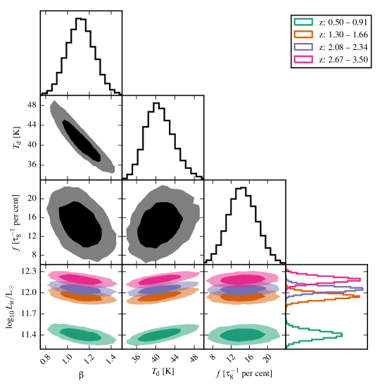
Figure 3: Contours of the 68 and 95 per cent credible intervals of the parameters for the quasar efficiency model in light and dark shades respectively. The histograms display each parameter’s marginalized posterior distribution. Parameters $f$, $\beta$ and $T_{\rm d}$ are fit globally across all redshift bins. For the other parameters each colour indicates the constraints from a single redshift bin. For clarity, we show the bin dependent parameters for a subset of the redshift bins used.

Table 3: Marginalized parameter constraints for the quasar feedback model

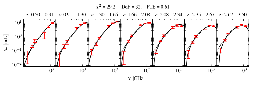
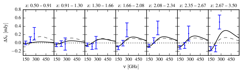
Figure 4: Top: stacked millimetre to infrared SEDs. Red data points represent the stacked data in our bands spanning 148–1200 GHz. The best-fitting stacked SEDs for the quasar feedback model for each redshift bin are shown in the solid black lines. The dotted black lines show the stacked model with no SZ effect. Bottom: dust subtracted millimetre SEDs highlighting the fit to the SZ component. The dust subtracted data are shown as the blue data points and the solid black lines represent the SZ component of the quasar feedback stacked model. The dashed grey lines shows the best-fitting SZ component when parameterized using the ${\smallint}p\mathrm{d}V$ formalism. The $\Delta S_{\nu}=0$ line, corresponding to a dust only signal is shown as the dotted black line. All errorbars shown here are statistical only and do not include the calibration uncertainties and covariances that are accounted for in the modelling.

Using the models outlined in Section 4.1, we fit the parameters $\beta$, $L_{\rm ir}^{\alpha}$, $T_{\rm d}$ and either ${\smallint}p\mathrm{d}V$ or $f$ where the $\alpha$ index labels each of our seven redshift bins.

For the ${\smallint}p\mathrm{d}V$ model, we find that the data are fit well with ${\smallint}p\mathrm{d}V=(2.2\pm 0.6)\times 10^{60}$ erg which corresponds to a total thermal energy of $E_{\rm th}=(6.2\pm 1.7)\times 10^{60}$ erg (using Equation 5). The fit yields $\chi^{2}$ = 36.3 for 32 degrees of freedom, resulting in a PTE of 0.28. For the quasar feedback model, we find $f=(14.5\pm 3.3)\tau_{8}^{-1}$ per cent with $\chi^{2}$ = 29.2 for 32 degrees of freedom, corresponding to a PTE of 0.61. Both of these models produce consistent best-fitting values for all the other parameters. For the quasar feedback model, the 68 and 95 per cent credible intervals for all the fit parameters are shown in Fig. 3 and their marginalized constraints are summarized in Table 4.2. The numbers in this table refer to the median of the marginalized parameter posteriors and the boundaries of their 68 per cent credible intervals. The maximum likelihood stacked SEDs from this model are shown along with the data in Fig. 4. In the lower plot of Fig. 4 we show the ACT data residuals, after subtracting the modelled dust SED. Overplotted is the best-fitting modelled SZ component. Both the ${\smallint}p\mathrm{d}V$ and quasar feedback models are shown.

These fits provide evidence for the presence of hot thermalized gas associated with these systems manifesting itself through an SZ distortion at millimetre wavelengths. A fit to the data explicitly neglecting the SZ component is formally worse than both of the above models with $\chi^{2}$ = 51.0 and 33 degrees of freedom. We therefore observe a $\Delta\chi^{2}$ improvement of 14.7 for the ${\smallint}p\mathrm{d}V$ model and 21.8 for the quasar feedback model, both of which add one additional parameter. This corresponds to $3\sigma$ evidence for the presence of associated thermalized gas or, assuming the quasar feedback scenario, $4\sigma$ evidence for the thermal coupling of quasars to their surrounding medium.

We find the best-fitting models require significant evolution of $L_{\rm ir}$ across the redshift range we probe, spanning the range $10^{11.4-12.2}~{}{\rm L}_{\odot}$. The implications of this measurement are discussed in Section 5.1. Fitting for a single temperature across all redshift bins, we find $T_{\rm d}=40\pm 3$ K. Allowing the dust temperatures to vary independently for each redshift bin yields values all consistent with this globally fit temperature and shows no detectable sign of redshift evolution.

The best fitting value of the dust emissivity index $\beta$ is found to be $1.12\pm 0.13$. This is on the low end of the theoretical range of $1<\beta<2$ as discussed further in Section 5.2. As this value for the emissivity index warrants further investigation and due to the systematic dependence of our results on the chosen form of the dust model, we explore a range of alternative dust models in Appendix C. These include dust models with values of $\beta$ fixed to values more commonly seen in the literature, as well as composite two temperature models and models with an optically thick dust spectrum. We find that a model with $\beta$ fixed to 1.6 produces an acceptable fit (PTE=0.16) to the data with 3$\sigma$ evidence for the SZ effect. A model with $\beta$ fixed to 1.8 does not fit the data well (PTE=0.01). Motivated by increasing evidence that high redshift dusty galaxies are characterized by an optically thick dust emission (Riechers et al., 2013; Huang et al., 2014), we evaluate a model with an optically thick dust component. This model fits the data (PTE=0.69) with $\beta=1.3\pm 0.3$ and 4$\sigma$ evidence for SZ. A two-temperature model adequately fits the data (PTE=0.35) with $\beta=1.4\pm 0.1$ (for both greybodies) and no SZ component. However, this model comes at the cost of significant additional model complexity in the form of seven additional parameters.

5 Discussion

Our data and modelling results establish that the far-infrared (FIR) and millimetre SEDs of radio-quiet quasars are (1) dominated by dust emission and (2) require at the 3$\sigma$–4$\sigma$ level an SZ distortion for most dust emission models. Insomuch as the bolometric FIR luminosity of quasars is the least model-dependent quantity in our analysis, we begin our discussion with $L_{\rm ir}$, its redshift evolution and associated star formation rates in Section 5.1. We then consider our best-fitting dust models in the context of previous studies in Section 5.2. For most of these models, an SZ effect is preferred. In Section 5.3, we consider whether the level of the SZ is consistent with simple virialization given the quasar host halo masses or whether energy injection from feedback should be invoked. Finally in Section 5.4, we compare our findings to other studies of the SZ effect associated with quasars and their hosts.

5.1 Infrared Luminosity and Star Formation Rates of Quasars

Our models provide estimates of the FIR luminosity of quasars through the $L_{\rm ir}$ parameters fit to our data in each redshift bin. The FIR emission associated with quasars originates from warm dust that is heated by ultraviolet radiation from young stars and the quasar itself. In the absence of detailed mid-infrared data, these contributions are difficult to separate. Kirkpatrick et al. (2012) attempt to quantify the percentage contribution due to star formation in these systems, finding 21 and 56 per cent of the FIR bolometric luminosity is due to star formation at $z\sim 1$ and $z\sim 2$, respectively. We instead estimate only upper limits on the star formation rates of quasar hosts by assuming no infrared contribution originating from quasar emission and using the total infrared bolometric luminosities of these systems to calculate their star formation rates. The $L_{\rm ir}$ values we report derive from the normalization of the greybody emission we model and therefore represent only a portion of the total infrared bolometric luminosities. To estimate the total infrared luminosity of star formation, $L^{\prime}_{\rm ir}$, we use the relationship between total $L^{\prime}_{\rm ir}$ and rest-frame 160 µmluminosity, $L_{160}$ from Symeonidis et al. (2008). For the redshift range we probe, this rest-frame frequency falls within the frequency coverage of our data. Using total $L^{\prime}_{\rm ir}$ calculated from $L_{160}$ values derived from the best-fitting SED models for each redshift bin, we obtain average star formation rates using the relation from Bell (2003). We find that the average star formation rates of quasar hosts are no more than $\sim 60,~{}250$ and $400~{}{\rm M}_{\odot}/{\rm yr}$ for $z\sim$1, 2 and 3, respectively.

5.2 Dust Emission Models

For both parameterizations of the SZ effect, the best-fitting values of the dust emissivity $\beta$ for an optically thin greybody model are found to be, $1.12\pm 0.13$. The turn over in the SEDs prefer a greybody model of temperature $T_{\rm d}\approx 40$ K, consistent with previous observations (Beelen et al., 2006; Dai et al., 2012). In Appendix C, we evaluate fits with alternative dust emission models with fixed emissivity, with optically thick emission, and with two dust components at different temperatures. All models require a component with temperature $T_{\rm d}\approx 40$ K. However the dust emissivities of these alternative models skew higher, giving 68 per cent credible regions with $\beta\lesssim 1.6$ and 95 per cent credible regions with $\beta\lesssim 1.8$. Given the preference for lower dust emissivities in these results, we review below studies relevant to this aspect of our dust models.

Millimetre-wavelength observations find $\beta$ to vary among different galaxies between the theoretical bounds ($1\leq\beta\leq 2$, Bohren & Huffman, 1983), peaking at $\beta=1.5$ (Carico et al., 1992; Lisenfeld et al., 2000). Herschel has revolutionized the study of FIR SEDs of extragalactic sources. A common assumption for fitting Herschel data is $\beta=1.5$ (Kirkpatrick et al., 2012), but because $\beta$ is only relevant for the Rayleigh-Jeans tail of the SED (i.e., at wavelengths well beyond that of the thermal peak) rarely does the wavelength coverage extend to long enough wavelengths to constrain $\beta$ from unrestricted fits, which is especially problematic because of the presence of components at a range of temperatures (Sun et al., 2014). Perhaps the most relevant comparison is with other sub-millimetre observations. For example, values of $\beta=1.3$, are observed by Planck in local star-forming galaxies (Negrello et al., 2013), consistent with spectral indices inferred by SPT in their high-$z$ dust dominated source population (Mocanu et al., 2013). In a sub-millimetre study of quasars, Beelen et al. (2006) find $\beta=1.6\pm 0.1$. These latter studies are broadly consistent with our results.

Additionally, all the models require a dominant component with temperature $\sim 40$ K. These temperature values apply only to the low-frequency emission; in practice, the SED of quasars is dominated by thermal components at much larger temperatures (Richards et al., 2006b), all the way to the dust sublimation cutoff at $T\ga 1000$ K. All higher temperature components produce $\nu^{2+\beta}$ spectra at the wavelengths of our Herschel-SPIRE and ACT observations; thus, our fits only recover the lowest temperature present in the multi-temperature distribution. While this higher temperature dust tends to affect the Wein side of the blackbody spectrum, a colder component could change the shape of the low-frequency spectrum. If there are such additional colder components at $T<40$ K, because of our single-temperature fitting procedure, they will tend to reduce the apparent $\beta$ (Dunne & Eales, 2001).

Finally, there is observational evidence that the SEDs of high-$z$ dusty star forming-galaxies are indicative of optically thick dust (Riechers et al., 2013; Huang et al., 2014). The precise origin of the dust emission of the quasar hosts is difficult to ascertain and the implicit assumption of dust optical depth $<<1$ in our fiducial dust models may not be justified. Allowing for an optically thick greybody spectrum has the effect of broadening the dust peak and would manifest itself as an artificially lower $\beta$ index when not accounted for.

5.3 Interpretation of the Observed SZ Signal

In Section 4.2, we show that the data favour (at the 3$\sigma$–4$\sigma$ level for most dust models) SED models for the stacked quasar sample with a thermal SZ contribution. We find that scaling this signal by the quasar bolometric luminosities, as expected if this energy is sourced by quasar feedback, provides a good fit to the data and yields a quasar feedback heating efficiency of $f=(14.5\pm 3.3)\tau_{8}^{-1}$ per cent. Formally, this percentage is an upper limit because some of the thermal energy responsible for the SZ effect is due to simple virialization, which is not included in the feedback model. However in the following we argue that most estimates of quasar host halo masses imply that the contribution from virialization is modest. Furthermore we cannot separately constrain the heating efficiency $f$ and the period of quasar activity $\tau$. Quasar lifetimes are quite poorly known (Martini, 2004), but we can use theoretical and observational estimates of quasar lifetimes from the literature to normalize our result to a fiducial value. Earlier observational estimates favoured $\tau\la 10^{8}$ yr (Martini & Weinberg, 2001; Jakobsen et al., 2003; Schirber et al., 2004; Shen et al., 2007; Worseck et al., 2007; Gonçalves et al., 2008; Trainor & Steidel, 2013) while more recent ones suggest $\tau\ga 10^{8}$ yr (Marconi et al., 2004; DiPompeo et al., 2014, 2015), with values $\sim 10^{8}$ yr commonly suggested by models of galaxy formation (Hopkins et al., 2005a, b). As, on average, we should observe a given quasar halfway through its active lifetime, the period of activity prior to observation should be estimated as the typical quasar lifetime divided by two. In addition to being systematically dependent on this quasar lifetime estimate, the efficiency values we derive also depend on the accuracy of our estimates of the optical bolometric luminosities for the sample. The bolometric corrections used to derive these values (see Appendix A) are uncertain at the 40 per cent level. The luminosity scaling of this signal is further explored in Appendix B.

In the literature, values of $\sim$5–7 per cent efficiency in thermalizing quasar radiative energy into the gas immediately around the accretion system are more typically used in galaxy formation and evolution models (e.g., Springel et al., 2005; Hopkins et al., 2006). Feedback in this form and with these efficiency values has been shown to bring both simulated and semi-analytic models of self-regulating quasar feedback in line with the observed $M_{\rm BH}$–$\sigma$ relation and quasar luminosity function (Wyithe & Loeb, 2003; Di Matteo et al., 2005). However, the thermalization efficiency remains poorly known and the exact value obtained from the simulations depends on the details of the feedback implementation (Ciotti & Ostriker, 2001; Novak et al., 2011; Choi et al., 2012).

While the quasar feedback model provides a compelling explanation for this SZ signal we also consider the possibility that this signal results in whole or in part from hot gas in virial equilibrium with the quasar host haloes, a more typical manifestation of the SZ effect such as that found in galaxy clusters (e.g., Hasselfield et al., 2013a; Bleem et al., 2015; Planck Collaboration et al., 2015). In a study of the SZ effect associated with radio-loud AGN, Gralla et al. (2014) find a signal consistent with that expected from the gravitationally shock heated ionized haloes of the massive ($\gtrsim 10^{13}$M_⊙) hosts of these objects. While not precisely known, the halo masses of the quasars in our study are expected to be significantly lower in mass. Galaxy-quasar clustering measurements at the lower limit of the redshift range we target ($z\sim 0.5$) yield quasar halo masses of $\sim 4\times 10^{12}h^{-1}$M_⊙ (Shen et al., 2013) with a weak dependence of halo mass on quasar bolometric luminosity. Quasar-quasar clustering on the other hand yields a halo mass of $\sim 1\times 10^{12}h^{-1}$M_⊙ at $z=2.4$ with no evidence for luminosity dependence (White et al., 2012). Wang et al. (2015) find that the cross-correlation signal between quasars and the CIB is well fit by a halo model for clustering corresponding to a host halo mass of $10^{12.36\pm 0.87}h^{-1}$M_⊙ for DR9 quasars with a median redshift of $2.5$. The quasars in the latter two of these clustering studies were optically selected type 1 objects in the SDSS-III survey, and are thus comparable samples to that used in our work. Somewhat higher halo mass values $\gtrsim 5\times 10^{12}h^{-1}$M_⊙ are found in clustering studies of $z\gtrsim 2$ unobscured quasars by Richardson et al. (2012) and CMB lensing studies such as Sherwin et al. (2012) and DiPompeo et al. (2014, 2015). The latter two of these measurements are not directly comparable to our work as they are based on infrared-selected quasars with photometric redshifts.

Taking a range of $(1-5)\times 10^{12}h^{-1}$M_⊙ we can estimate the expected magnitude of the SZ signal due only to the gravitationally heated virialized reservoirs of hot gas that would be associated with haloes of this mass. Planck Collaboration et al. (2013) find that the integrated SZ signal,

$$Y\equiv\int y~{}\mathrm{d}\Omega=\frac{\sigma_{\rm T}}{m_{\rm e}c^{2}}\frac{\smallint p\mathrm{d}V}{D^{2}_{\rm A}(z)},$$ (10)

of $z<1$ quiescent galaxies closely traces the simple self-similar scaling with halo mass,

$$Y~{}E^{-2/3}(z)~{}\left(\frac{D_{\mathrm{A}}(z)}{500~{}\mathrm{Mpc}}\right)^{2}=(2.9\pm 0.3)\times 10^{-8}\mathrm{arcmin}^{2}\left(\frac{M_{\mathrm{h}}}{10^{12}\mathrm{M}_{\odot}}\right)^{5/3}$$ (11)

down to a halo mass of $\sim 3\times 10^{13}$M_⊙. Broad agreement with this scaling relation is found in Gralla et al. (2014) when comparing the magnitude of their SZ signal to the expected halo mass of radio-loud AGN hosts. The Planck study gives this relation using the quantities $Y_{500}$ and $M_{500}$, defined with respect to a physical radius $R_{500}$ enclosing a mean density of $500\rho_{\rm c}(z)$ (see also Le Brun et al., 2015). In Equation 11, we have accounted for a factor of $Y/Y_{500}\approx 1.8$, where $Y$ corresponds to the total integrated SZ signal. This factor is calculated using the same universal radial pressure profile from Arnaud et al. (2010) as is used in Planck Collaboration et al. (2013). A factor of $M_{\rm h}/M_{500}=1.6$ is used, consistent with the conversion from $M_{500}$ to $M_{200}$ from the concentration relation of Duffy et al. (2008). This yields a closer proxy of the halo virial mass referred to here as $M_{\mathrm{h}}$. We assume the entirety of the signal we observe is enclosed within the ACT beams such that $Y$, the total integrated signal is what our data constrain. This is a reasonable assumption as $R_{200}$ for a $5\times 10^{12}h^{-1}$M_⊙ halo corresponds to 0.4 arcmin (within the ACT beam scales) at $z=1.85$, the median redshift of our sample. Explicitly correcting for the band dependent beam dilution effect for an SZ signal of this scale would require a model dependent choice of SZ profile and result in corrections small relative to the measurement uncertainties. Combining Equation 10 and Equation 11, we find

$$\frac{\smallint p\mathrm{d}V}{10^{60}\mathrm{erg}}\approx 0.011~{}E^{2/3}(z)\left(\frac{M_{\mathrm{h}}}{10^{12}~{}\mathrm{M}_{\odot}}\right)^{5/3}.$$ (12)

While many of the assumptions made in deriving this relation may not hold for quasar hosts, these arguments provide a rough estimate of the ${\smallint p\mathrm{d}V}$ signal one would expect from purely gravitationally thermalized gas reservoirs hosted in these systems. For quasar halo masses in the range $(1-5)\times 10^{12}h^{-1}$M_⊙ we find the expected level of this signal to be ${\smallint p\mathrm{d}V}=(0.4$–$5.8)\times 10^{59}$ erg at the median redshift of our catalogue, $z=1.85$. Thus these purely gravitational arguments under predict our measured result of ${\smallint p\mathrm{d}V}=(2.2\pm 0.6)\times 10^{60}$ erg making up at most $\sim$30 per cent of the signal we observe, depending on the choice of halo mass. Given this amount of thermal energy the gas in these haloes could either be gravitationally bound or unbound, again depending on the value taken for the halo mass.

The validity of this calculation is dependent on the details of the high-mass tail of the halo mass distribution of quasar hosts. Since in the case of gravitational heating, the SZ contribution of each host halo is proportional to $M^{5/3}$, the effective mass that should be used in Equation 12 is $\langle M^{5/3}\rangle^{3/5}$ where the average is taken over the mass distribution of quasar host haloes. How much higher this effective mass is compared to the halo masses we take from the literature depends on the behaviour of the high-mass tail of this distribution. As an example of how this can affect the interpretation of these results, we analytically approximate the average quasar host halo mass distribution of the $z\sim 1.4$ sample of the Richardson et al. (2012) clustering study. Using this approximation for the full mass distribution and calculating $\langle M^{5/3}\rangle^{3/5}$, we find that the effective mass scale corresponds to an expected signal from purely gravitational arguments of ${\smallint p\mathrm{d}V}\sim 4\times 10^{60}$ erg. Unfortunately, the high-mass end of the quasar halo mass distribution, upon which this calculation relies, is not well constrained (Richardson et al., 2012; Shen et al., 2013). Shen et al. (2013) find that data from clustering studies can be fit equally well by models with very different parameterizations for the mass dependence of the quasar halo occupation distribution, demonstrating the model dependent nature of results for halo mass distribution in the literature (including the relative contribution of correlated high-mass haloes to these studies). We therefore do not attempt to correct for this in our primary discussion.

5.4 Comparison with Other Studies

Recently Ruan et al. (2015) published a detection of quasar feedback in the Planck data at the level of $E_{\rm th}=10^{62}$ erg, over an order of magnitude larger than one would expect from the physical arguments presented here and what we measure. This level of SZ effect is characteristic of the galaxy group mass scale and would leave a clear decrement at the level of several mJy around each quasar in 150 GHz data from ACT and the SPT. Such a signal is challenged by both source studies, such as our own, and power spectrum studies with ACT data (Dunkley et al., 2013; Sievers et al., 2013). Furthermore, it appears that the feedback efficiency of 0.05 reported in Ruan et al. (2015) is not computed as a fraction of a single accretion event’s energy, as in our formalism, but rather as a fraction of the total black hole rest mass energy. An energy of $10^{62}$ erg would correspond to essentially 100 per cent efficient feedback. Another issue with this level of $E_{\rm th}$ is that it exceeds the binding energy ($E_{\rm b}\approx 2.5\times 10^{59}~{}{\rm erg}~{}(M_{\rm h}/10^{12}~{}{\rm M}_{\odot})^{5/3}E^{2/3}(z)$) of the host haloes.

Chatterjee et al. (2010) correlated WMAP 5-Year data at 40, 60, and 90 GHz with a large photometric catalogue of quasars from the SDSS Data Release 3. They reported a 2.5$\sigma$ flux decrement at 40 GHz and estimated a mJy integrated SZ effect from a two parameter fit (SZ and dust) to their three-band SED. While this amplitude is not dissimilar to that found here, Chatterjee et al. (2010) in their discussion noted the difficulty of establishing a firm conclusion about the nature of their measurement given the limited frequency coverage, sensitivity and resolution of the millimetre data. In particular, significant systematic effects were associated with the choice of foreground treatment and data selection, likely resulting in observed systematics at low frequency where much of their detection significance was derived (cf. figs 7.12–15 of Chatterjee, 2009).

Cen & Safarzadeh (2015b) uses a halo catalogue from the Millenium simulation with analytic prescriptions for identifying quasar hosts (outlined in Cen & Safarzadeh (2015a)) and constructing an associated Compton-$y$ map. Their study demonstrates that contaminating projected SZ signal from two halo correlations is important to account for in quasar stacking studies, particularly for large beam sizes, $\sim 10$ arcmin. This effect is less important for higher resolution, $\sim 1$ arcmin (similar to the ACT beam scale) studies but may need to be modelled in future work. Additionally they find that such high-resolution studies may be promising in constraining models for the quasar halo occupation distribution.

During the final stage of preparing this document, Verdier et al. (2015) submitted a similar study of the SDSS DR12 quasar catalogue using 70–857 GHz data from the Planck satellite. Their measured SZ amplitude is broadly consistent with that found in this work, however, there are some differences in the quasar dust properties and interpretation of the SZ effect.

6 Conclusions

Using a stacking analysis of ACT and Herschel data with the SDSS spectroscopic quasar catalogue we reconstruct millimetre and FIR SEDs of quasars spanning the redshift range $0.5<z<3.5$. We fit these data with a model for the stacked SED incorporating a dust component that is allowed to evolve as a function of redshift as well as an SZ distortion. Our conclusions are as follows:

• While the observed signal is dust dominated, 3$\sigma$–4$\sigma$ evidence is found for the thermal SZ effect associated with these systems for most dust models. In Appendix C, we explore the effects of alternative dust parameterizations on this result.

• This observed SZ signal is consistent with the scenario that this energy is being fuelled by quasar feedback in which up to $(14.5\pm 3.3)\tau_{8}^{-1}$ per cent of the quasar radiative energy is thermalized in the surrounding medium.

• Fitting for the typical thermal energy associated with quasars, we find a best-fitting value of $E_{\rm th}=(6.2\pm 1.7)\times 10^{60}$ erg. This exceeds by an order of magnitude what would be expected for a gravitationally heated circumgalactic medium for the $(1-5)\times 10^{12}h^{-1}$M_⊙ haloes quasars are though to occupy. However, if correct, the highest quasar halo mass estimates found in the literature could explain a large fraction of the observed SZ effect with purely gravitational heating.

• Using the relation from Symeonidis et al. (2008) and the rest-frame 160 µm luminosities from our SED models, we determine upper limits for the average star formation rates of quasar hosts of $\sim 60,~{}250$ and $400~{}{\rm M}_{\odot}/{\rm yr}$ for $z\sim$1, 2 and 3, respectively.

Forthcoming, deeper and wider ACT data will provide more precise estimates for the SEDs in the millimetre but without a better understanding of the halo masses and dust properties of high redshift quasar hosts, future studies will remain limited by associated systematics in the interpretation of the improved constraints.

Acknowledgements

We thank the anonymous referee for their useful comments and suggestions. This work was supported by the US National Science Foundation through awards AST-0408698 and AST-0965625 for the ACT project, as well as awards PHY-0855887 and PHY-1214379. Funding was also provided by Princeton University, the University of Pennsylvania, and a Canada Foundation for Innovation (CFI) award to UBC. ACT operates in the Parque Astronómico Atacama in northern Chile under the auspices of the Comisión Nacional de Investigación Científica y Tecnológica de Chile (CONICYT). Computations were performed on the GPC supercomputer at the SciNet HPC Consortium. SciNet is funded by the CFI under the auspices of Compute Canada, the Government of Ontario, the Ontario Research Fund – Research Excellence; and the University of Toronto. We acknowledge the use of the Legacy Archive for Microwave Background Data Analysis (LAMBDA), part of the High Energy Astrophysics Science Archive Center (HEASARC). HEASARC/LAMBDA is a service of the Astrophysics Science Division at the NASA Goddard Space Flight Center. This research made use of Astropy, a community-developed core python package for Astronomy (Astropy Collaboration et al., 2013) and the affine invariant MCMC ensemble sampler implementation provided by the emcee python package (Foreman-Mackey et al., 2013).

Appendix A Optical Bolometric Luminosity Determination

As we investigate models that assume the thermal energy we observe through the SZ effect is dominated by converted quasar radiative energy (see the quasar feedback model described in Section 4), we additionally construct estimates for the optical bolometric luminosity, $L_{\rm bol}$, of each of the quasars in this sample. For this purpose we again make use of SDSS $i$-band absolute magnitudes, $\mathcal{M}_{I}(z=2)$ which are converted to rest-frame luminosities $L_{2500}$ at 2500 Å and then to $L_{\rm bol}$ by applying the bolometric correction from Richards et al. (2006a). These estimated bolometric luminosities are shown in Fig. 5. Since the DR10 survey was designed to target quasars at $z>2$ its fainter magnitude limit ($i<20.5$) yields an increase in lower luminosity quasars at high redshift (Pâris et al., 2014) observed as the discontinuity at $z\sim 2$ in Fig. 5.

The bolometric correction varies in a systematic way as a function of luminosity and colour of the quasar but these variations among the different sub-populations do not exceed 15% (Richards et al., 2006a). There are, however, systematic concerns in constructing these estimates. In particular, double counting direct ultraviolet emission by also including re-radiated dust emission when integrating the SED used to derive these values can lead to overestimation of the correction. By restricting the integral of the SED to the range between 1µm and 2 keV, Krawczyk et al. (2013) obtain a bolometric correction of 2.75 from the 2500Å monochromatic luminosity compared to the value of 5 from Richards et al. (2006a), providing a lower bound on the bolometric correction. Krawczyk et al. (2013) further explore a range of models and observations for the ultraviolet and X-ray spectra of quasars finding bolometric corrections from 2500Å to lie between 2.75 and 5. Using a different sample and different methods, Marconi et al. (2004) calculate bolometric corrections from $B$ band to be between 5 and 7, a value which weakly depends on quasar luminosity. Applying the Vanden Berk et al. (2001) power-law slope to correct these to 2500Å, we find bolometric corrections between 3.6 and 5.1. A similar procedure yields a range of bolometric corrections between 3.6 and 7.3 for the Elvis et al. (1994) SED. While we make use of the Richards et al. (2006a) bolometric correction we note that these values are still not known to better than 40 per cent, which systematically affects the interpretation of our SZ constraints on quasar feedback.

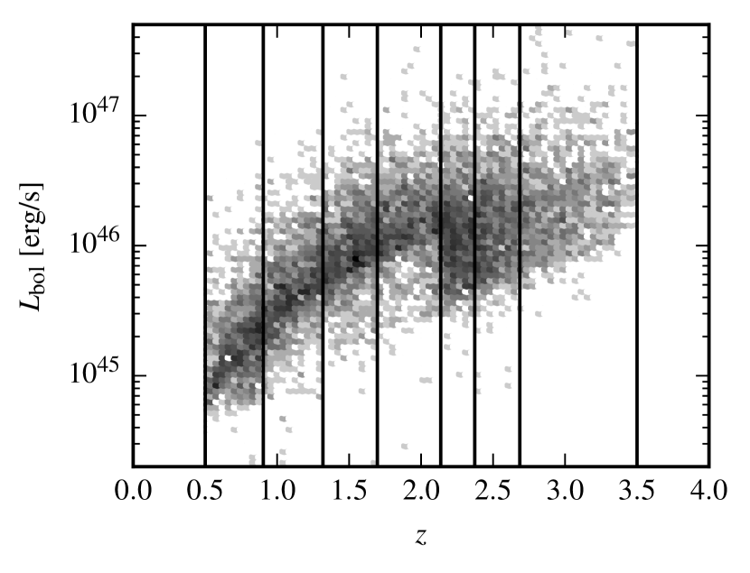
Figure 5: The optical bolometric luminosity–redshift distribution of combined SDSS DR7 and DR10 spectroscopic quasar sample falling within the ACT equatorial region ($-55\degr\leq\alpha\leq 58\degr$, $-1\aas@@fstack{\circ}5\leq\delta\leq 1\aas@@fstack{\circ}5$) after the radio-loud cut has been applied. The density grey-scale used is logarithmic and the vertical black lines denote the boundaries of the redshift bins we use for the stacking analysis. The optical bolometric luminosity–redshift distribution of the subset of our sample which lies within the HerS region is found to be similar.

Appendix B Optical Luminosity Dependence

The feedback interpretation of the SZ signal operates under the assumption that a fraction of the bolometric luminosity of these sources is being converted to thermal energy which we observe through the SZ effect. This therefore implies that the most bolometrically luminous sources should dominate in their contribution to our observed SZ distortion. This luminosity dependence is explicitly accounted for in the quasar feedback model but in this appendix we explore an alternative means of measuring this dependence by evaluating the effect of luminosity cuts in the quasar catalogue on the SZ amplitude extracted from fitting to the ${\smallint}p\mathrm{d}V$ model. Simply cutting the 8435 objects with optical bolometric luminosity $L_{\rm bol}>1\times 10^{46}$ erg (determined as described in Appendix A) we find that the best-fitting ${\smallint}p\mathrm{d}V$ shifts from $(2.2\pm 0.6)\times 10^{60}$ erg to $(1.3\pm 0.6)\times 10^{60}$ erg. However, a naïve cut such as this may produce biased results as it significantly alters the sample’s redshift distribution due to the strong redshift dependence of the optical bolometric luminosities (See Fig. 5). We therefore perform a further test by selecting a range of redshift, $2.1<z<3.0$, over which the luminosity distribution remains qualitatively similar. The objects falling within this range are separated into two bins of bolometric luminosity, each of which is fit with a model including greybody dust and an SZ component parameterized through ${\smallint}p\mathrm{d}V$. We find that for the low luminosity bin ($L_{\rm bol}<10^{46.3}$ erg) the best-fitting SZ amplitude is ${\smallint}p\mathrm{d}V=2.2\pm 1.1\times 10^{60}$ erg, whereas for the $L_{\rm bol}>10^{46.3}$ erg bin we find ${\smallint}p\mathrm{d}V=4.4\pm 1.8\times 10^{60}$ erg, again demonstrating a marginal shift to higher SZ amplitude for higher luminosity objects.

Appendix C Alternative Dust Models

The significance of the SZ effect depends on the marginalization of the parameters of the assumed dust model in the fits. In this appendix we explore some alternative dust models and report how the choice of dust model affects the SZ detection and the goodness of fit to the data. A summary of these fits to alternative models is provided in Table 4.

Table 4: Summary of fitting results for fiducial models as well as models with alternative dust treatments.

Model description	DoF	$\chi^{2}$	PTE	$\Delta{\rm DoF}_{\rm ref}$$a$	$\Delta\chi^{2}_{\rm ref}$$a$
Fiducial models
Greybody only	33	51.0	0.02	0	0
Quasar feedback	32	29.2	0.61	1	21.8
${\smallint}p\mathrm{d}V$	32	36.3	0.28	1	14.7
Alternative quasar feedback models
Fixed $\beta$ $b$
$\quad\quad\beta=1.6$	33	41.8	0.14	0	9.2
$\quad\quad\beta=1.8$	33	53.3	0.01	0	-2.3
Optically thick	31	26.7	0.69	2	24.3
Alternative dust only models
Two temperature	26	28.1	0.36	7	22.9
Broken power law	31	39.4	0.14	2	11.6

• These values correspond to the reduction in degrees of freedom and $\chi^{2}$ of each model with respect to the reference model which is the fit with no SZ effect and a single temperature greybody dust spectrum (the “Greybody Only" model).

• These models are found to still prefer non-zero values at the $\sim 3\sigma$ level in their marginalized constraints for the SZ amplitude. The negative $\Delta\chi^{2}_{\rm ref}$ for the $\beta=1.8$ model indicates it is a poorer fit than the reference greybody only model.

C.1 Fixed $\beta$ models

In order to understand the effect of taking the dust emissivity index $\beta$ as a free parameter in our fits, we attempt fits with the value of $\beta$ fixed. As can be seen in Fig. 3, there is degeneracy between the best-fitting value of $\beta$ and the efficiency of quasar feedback, parameterized through $f$. A similar degeneracy is seen in the ${\smallint}p\mathrm{d}V$ model where, when fitting, the amplitude of the SZ signal is inversely proportional to the fit value for $\beta$. In Section 5.2 we noted that our fit value of $\beta$ is on the low end of the theoretically allowed range of 1–2, further motivating a check using models with values more commonly seen in the literature. We perform the same modelling of the stacked fluxes as described in Section 4 but instead of allowing $\beta$ as a free parameter we hold its value fixed. We use the quasar feedback parameterization for the SZ effect here. Motivated by the results of Beelen et al. (2006) and Hardcastle et al. (2013) respectively, we fit models with $\beta$ fixed to values of 1.6 and 1.8. As expected, these models produce worse $\chi^{2}$ values than models in which $\beta$ is a free parameter as shown in Table 4. The model with $\beta=1.6$ provides an adequate fit to the data with a PTE of 0.14. The $\beta=1.8$ model provides a considerably poorer fit with a PTE of 0.01. However, while detected at a lower amplitude ($f\approx 8.5~{}\tau_{8}^{-1}$ per cent) the marginal constraints on the SZ amplitude for both of these fixed $\beta$ models prefer non-zero values at the $\sim 3\sigma$ level.

C.2 Optically Thick Model

We evaluate the effect of the assumption of dust optical depth $<<1$ implicit in our fiducial dust SEDs by fitting the data with a model where we allow for an optically thick component. The corresponding dust SED for this optically thick model is

$$S_{\rm dust}(\nu,z,L_{\rm ir},\tau_{0},\beta,T_{\rm d}) =\frac{L_{\rm ir}}{4\pi D_{\rm L}^{2}(z)}\frac{\phi((1+z)\nu)}{\int\phi(\nu^{\prime})\mathrm{d}\nu^{\prime}}$$ (13)

$$\phi(\nu) =(1-\mathrm{e}^{-\tau_{0}(\nu/\nu_{100\mu})^{\beta}})B_{\nu}(T),$$ (14)

where, $\nu_{100\mu}$ is defined such that $\tau_{0}$ represents the dust optical depth at rest-frame wavelength of 100 µm. We fit the data with $\tau_{0},~{}\beta$ and $T_{\rm d}$ as the globally fit dust parameters and use the quasar feedback parameterization of the SZ effect. We find this model provides a good fit to the data (as summarized in Table 4) with $\chi^{2}=26.7$ for 31 degrees of freedom, corresponding to a PTE of 0.69. Constraints on the SZ effect, parameterized through $f$ are found to be unchanged. The dust opacity is not well constrained with $\log_{10}{\tau_{0}}=0.2^{+2.2}_{-0.5}$ but we find the expected positive correlation between dust optical depth and dust emissivity index $\beta$ due to the broadening of the dust SED peak provided by the optically thick model.

The marginalized best-fitting emissivity index for this model is $\beta=1.3\pm 0.3$ and the dust temperature, $T_{\rm d}=52\pm 11$ K, is constrained to values centred higher but still consistent with those determined in the optically thin models.

C.3 Two Temperature Model

In this section, we examine whether the interpreted SZ distortion could instead be the result of an additional lower temperature dust component contributing to the SED at frequencies below the primary greybody peak. To test this, we attempt a model with no SZ component and a dust component that is made up of the sum of two greybody SEDs. Such models were found to be highly degenerate in the parameters describing the two dust components. To overcome some of this degeneracy we fix the temperature of the primary (high temperature) dust component to 40 K, consistent with what we find in the quasar feedback and ${\smallint}p\mathrm{d}V$ models. We then fit for a single value for the temperature of the cold dust component across all redshift bins, restricting it to be $<30$ K with a truncated uniform prior. We fit the amplitudes of both components, parameterized through their infrared bolometric luminosity, $L_{\rm ir}$ as defined in Section 4, on a bin by bin basis. We find that the resulting best-fitting model provides a good fit to the data with a $\chi^{2}=28.1$ for 26 degrees of freedom, corresponding to the PTE of 0.35. The best-fitting value for the temperature of the cold dust component corresponds to $20\pm 3$ K and the bolometric luminosities for this component range from $10^{10.7-11.4}$ L_⊙, increasing with redshift. This two temperature model cannot be ruled out as an alternative explanation for the signal we observe. However (as shown in Table 4) this reduction in $\chi^{2}$ of 22.9 with respect to the reference greybody dust only model comes at the expense of seven additional parameters, whereas both SZ models are significantly less complex, producing comparable $\chi^{2}$ reductions for a single additional parameter. Applying the Bayesian information criterion (BIC), a test that explicitly penalizes additional model complexity, we find a $\Delta$BIC improvement of $>$10. This corresponds to “strong evidence" against the preference of this two temperature model over the quasar feedback model based on this criterion.

C.4 Broken power-law Model

We additionally attempt fits using a dust model that has two emissivity indices, such that the dust spectrum takes the form of a broken power law at low frequencies.

The modelled dust spectrum then becomes

$$S_{\rm dust}(\nu,z,L_{\rm ir},\nu_{\rm b},\beta_{0},\beta_{1},T_{\rm d})=\frac{L_{\rm ir}}{4\pi D_{\rm L}^{2}(z)}\frac{\phi((1+z)\nu)}{\int\phi(\nu^{\prime})\mathrm{d}\nu^{\prime}}$$ (16)

$$\phi(\nu)=\begin{cases}(\nu/\nu_{\rm b})^{\beta_{0}}B_{\nu}(T_{\rm d})\ {\rm for}\ \nu\leq\nu_{\rm b}\\ (\nu/\nu_{\rm b})^{\beta_{1}}B_{\nu}(T_{\rm d})\ {\rm for}\ \nu>\nu_{\rm b}\\ \end{cases},$$ (17)

where $\nu_{\rm b}$ parameterizes the location of the spectral break with $\beta_{0}$ and $\beta_{1}$ parameterizing the emissivity index above and below this break respectively. We fit a model with only a dust component of this form to determine whether the SZ distortion we measure could instead be explained by such a spectrum. In this model, we fit single values for $\nu_{\rm b},\ \beta_{0},\ \beta_{1}$ and $T_{\rm d}$ while the $L_{\rm ir}$ values are fit independently on a bin by bin basis. As shown in Table 4, the resulting $\chi^{2}$ of 39.4 with 31 degrees of freedom (corresponding to a PTE of 0.14) indicates an adequate fit to the data. However, the best-fitting constraints on the emissivity indices are found to be $\beta_{0}=1.52^{+0.21}_{-0.25}$ and $\beta_{1}=0.25^{+0.18}_{-0.31}$ with the rest-frame spectral break at $\nu_{\rm b}=1250^{+170}_{-210}$ GHz. This value for $\beta_{1}$ is well outside the theoretically allowed region of $1<\beta<2$ as discussed in Section 5.2 and therefore we reject this fit as less likely on physical grounds.

References

- Alexander et al. (2010) Alexander D. M., Swinbank A. M., Smail I., McDermid R., Nesvadba N. P. H., 2010, MNRAS, 402, 2211
- Arav et al. (2008) Arav N., Moe M., Costantini E., Korista K. T., Benn C., Ellison S., 2008, ApJ, 681, 954
- Arnaud et al. (2010) Arnaud M., Pratt G. W., Piffaretti R., Böhringer H., Croston J. H., Pointecouteau E., 2010, A&A, 517, A92
- Astropy Collaboration et al. (2013) Astropy Collaboration et al., 2013, A&A, 558, A33
- Battaglia et al. (2012) Battaglia N., Bond J. R., Pfrommer C., Sievers J. L., 2012, ApJ, 758, 74
- Becker et al. (1995) Becker R. H., White R. L., Helfand D. J., 1995, ApJ, 450, 559
- Beelen et al. (2006) Beelen A., Cox P., Benford D. J., Dowell C. D., Kovács A., Bertoldi F., Omont A., Carilli C. L., 2006, ApJ, 642, 694
- Begelman & Cioffi (1989) Begelman M. C., Cioffi D. F., 1989, ApJ, 345, L21
- Bell (2003) Bell E. F., 2003, ApJ, 586, 794
- Best & Heckman (2012) Best P. N., Heckman T. M., 2012, MNRAS, 421, 1569
- Bleem et al. (2015) Bleem L. E., et al., 2015, ApJS, 216, 27
- Bohren & Huffman (1983) Bohren C. F., Huffman D. R., 1983, Absorption and scattering of light by small particles
- Boyle & Terlevich (1998) Boyle B. J., Terlevich R. J., 1998, MNRAS, 293, L49
- Brusa et al. (2015a) Brusa M., et al., 2015a, MNRAS, 446, 2394
- Brusa et al. (2015b) Brusa M., et al., 2015b, A&A, 578, A11
- Cano-Díaz et al. (2012) Cano-Díaz M., Maiolino R., Marconi A., Netzer H., Shemmer O., Cresci G., 2012, A&A, 537, L8
- Carico et al. (1992) Carico D. P., Keene J., Soifer B. T., Neugebauer G., 1992, PASP, 104, 1086
- Carniani et al. (2015) Carniani S., et al., 2015, A&A, 580, A102
- Cen & Safarzadeh (2015a) Cen R., Safarzadeh M., 2015a, ApJ, 798, L38
- Cen & Safarzadeh (2015b) Cen R., Safarzadeh M., 2015b, ApJ, 809, L32
- Chatterjee (2009) Chatterjee S., 2009, PhD thesis, University of Pittsburgh
- Chatterjee & Kosowsky (2007) Chatterjee S., Kosowsky A., 2007, ApJ, 661, L113
- Chatterjee et al. (2008) Chatterjee S., Di Matteo T., Kosowsky A., Pelupessy I., 2008, MNRAS, 390, 535
- Chatterjee et al. (2010) Chatterjee S., Ho S., Newman J. A., Kosowsky A., 2010, ApJ, 720, 299
- Choi et al. (2012) Choi E., Ostriker J. P., Naab T., Johansson P. H., 2012, ApJ, 754, 125
- Ciotti & Ostriker (2001) Ciotti L., Ostriker J. P., 2001, ApJ, 551, 131
- Crenshaw et al. (2003) Crenshaw D. M., Kraemer S. B., George I. M., 2003, ARA&A, 41, 117
- Croton et al. (2006) Croton D. J., et al., 2006, MNRAS, 365, 11
- Dai et al. (2012) Dai Y. S., et al., 2012, ApJ, 753, 33
- Di Matteo et al. (2005) Di Matteo T., Springel V., Hernquist L., 2005, Nature, 433, 604
- DiPompeo et al. (2014) DiPompeo M. A., Myers A. D., Hickox R. C., Geach J. E., Hainline K. N., 2014, MNRAS, 442, 3443
- DiPompeo et al. (2015) DiPompeo M. A., Myers A. D., Hickox R. C., Geach J. E., Holder G., Hainline K. N., Hall S. W., 2015, MNRAS, 446, 3492
- Duffy et al. (2008) Duffy A. R., Schaye J., Kay S. T., Dalla Vecchia C., 2008, MNRAS, 390, L64
- Dunkley et al. (2013) Dunkley J., et al., 2013, J. Cosmology Astropart. Phys, 7, 25
- Dunne & Eales (2001) Dunne L., Eales S. A., 2001, MNRAS, 327, 697
- Dünner et al. (2013) Dünner R., et al., 2013, ApJ, 762, 10
- Eisenstein et al. (2011) Eisenstein D. J., et al., 2011, AJ, 142, 72
- Elvis et al. (1994) Elvis M., et al., 1994, ApJS, 95, 1
- Fabbri (1981) Fabbri R., 1981, Ap&SS, 77, 529
- Fabian (2012) Fabian A. C., 2012, ARA&A, 50, 455
- Faucher-Giguère & Quataert (2012) Faucher-Giguère C.-A., Quataert E., 2012, MNRAS, 425, 605
- Ferrarese & Merritt (2000) Ferrarese L., Merritt D., 2000, ApJ, 539, L9
- Foreman-Mackey et al. (2013) Foreman-Mackey D., Hogg D. W., Lang D., Goodman J., 2013, PASP, 125, 306
- Fowler et al. (2007) Fowler J. W., et al., 2007, Appl. Opt., 46, 3444
- Fu & Stockton (2009) Fu H., Stockton A., 2009, ApJ, 690, 953
- Gallagher et al. (2007) Gallagher S. C., Hines D. C., Blaylock M., Priddey R. S., Brandt W. N., Egami E. E., 2007, ApJ, 665, 157
- Gebhardt et al. (2000) Gebhardt K., et al., 2000, ApJ, 539, L13
- Gonçalves et al. (2008) Gonçalves T. S., Steidel C. C., Pettini M., 2008, ApJ, 676, 816
- Gralla et al. (2014) Gralla M. B., et al., 2014, MNRAS, 445, 460
- Greco et al. (2015) Greco J. P., Hill J. C., Spergel D. N., Battaglia N., 2015, ApJ, 808, 151
- Greene et al. (2011) Greene J. E., Zakamska N. L., Ho L. C., Barth A. J., 2011, ApJ, 732, 9
- Greene et al. (2014) Greene J. E., Pooley D., Zakamska N. L., Comerford J. M., Sun A.-L., 2014, ApJ, 788, 54
- Griffin et al. (2010) Griffin M. J., et al., 2010, A&A, 518, L3
- Griffin et al. (2013) Griffin M. J., et al., 2013, MNRAS, 434, 992
- Hainline et al. (2013) Hainline K. N., Hickox R., Greene J. E., Myers A. D., Zakamska N. L., 2013, ApJ, 774, 145
- Hainline et al. (2014) Hainline K. N., Hickox R. C., Greene J. E., Myers A. D., Zakamska N. L., Liu G., Liu X., 2014, ApJ, 787, 65
- Hajian et al. (2011) Hajian A., et al., 2011, ApJ, 740, 86
- Hand et al. (2011) Hand N., et al., 2011, ApJ, 736, 39
- Hardcastle et al. (2013) Hardcastle M. J., et al., 2013, MNRAS, 429, 2407
- Harrison et al. (2014) Harrison C. M., Alexander D. M., Mullaney J. R., Swinbank A. M., 2014, MNRAS, 441, 3306
- Harrison et al. (2015) Harrison C. M., Thomson A. P., Alexander D. M., Bauer F. E., Edge A. C., Hogan M. T., Mullaney J. R., Swinbank A. M., 2015, ApJ, 800, 45
- Hasselfield et al. (2013a) Hasselfield M., et al., 2013a, J. Cosmology Astropart. Phys, 7, 8
- Hasselfield et al. (2013b) Hasselfield M., et al., 2013b, ApJS, 209, 17
- Heckman et al. (1990) Heckman T. M., Armus L., Miley G. K., 1990, ApJS, 74, 833
- Hopkins et al. (2005a) Hopkins P. F., Hernquist L., Martini P., Cox T. J., Robertson B., Di Matteo T., Springel V., 2005a, ApJ, 625, L71
- Hopkins et al. (2005b) Hopkins P. F., Hernquist L., Cox T. J., Di Matteo T., Martini P., Robertson B., Springel V., 2005b, ApJ, 630, 705
- Hopkins et al. (2006) Hopkins P. F., Hernquist L., Cox T. J., Di Matteo T., Robertson B., Springel V., 2006, ApJS, 163, 1
- Hopkins et al. (2008) Hopkins P. F., Hernquist L., Cox T. J., Kereš D., 2008, ApJS, 175, 356
- Huang et al. (2014) Huang J.-S., et al., 2014, ApJ, 784, 52
- Jakobsen et al. (2003) Jakobsen P., Jansen R. A., Wagner S., Reimers D., 2003, A&A, 397, 891
- Kirkpatrick et al. (2012) Kirkpatrick A., et al., 2012, ApJ, 759, 139
- Krawczyk et al. (2013) Krawczyk C. M., Richards G. T., Mehta S. S., Vogeley M. S., Gallagher S. C., Leighly K. M., Ross N. P., Schneider D. P., 2013, ApJS, 206, 4
- Le Brun et al. (2015) Le Brun A. M. C., McCarthy I. G., Melin J.-B., 2015, MNRAS, 451, 3868
- Lisenfeld et al. (2000) Lisenfeld U., Isaak K. G., Hills R., 2000, MNRAS, 312, 433
- Liu et al. (2013a) Liu G., Zakamska N. L., Greene J. E., Nesvadba N. P. H., Liu X., 2013a, MNRAS, 430, 2327
- Liu et al. (2013b) Liu G., Zakamska N. L., Greene J. E., Nesvadba N. P. H., Liu X., 2013b, MNRAS, 436, 2576
- Mac Low et al. (1994) Mac Low M.-M., McKee C. F., Klein R. I., Stone J. M., Norman M. L., 1994, ApJ, 433, 757
- Magorrian et al. (1998) Magorrian J., et al., 1998, AJ, 115, 2285
- Mandelbaum et al. (2009) Mandelbaum R., Li C., Kauffmann G., White S. D. M., 2009, MNRAS, 393, 377
- Marconi et al. (2004) Marconi A., Risaliti G., Gilli R., Hunt L. K., Maiolino R., Salvati M., 2004, MNRAS, 351, 169
- Marsden et al. (2009) Marsden G., et al., 2009, ApJ, 707, 1729
- Marsden et al. (2014) Marsden D., et al., 2014, MNRAS, 439, 1556
- Martini (2004) Martini P., 2004, in Ho L. C., ed., in Coevolution of Black Holes and Galaxies (Cambridge: Cambridge University Press). p. 169
- Martini & Weinberg (2001) Martini P., Weinberg D. H., 2001, ApJ, 547, 12
- McNamara & Nulsen (2007) McNamara B. R., Nulsen P. E. J., 2007, ARA&A, 45, 117
- Mocanu et al. (2013) Mocanu L. M., et al., 2013, ApJ, 779, 61
- Moe et al. (2009) Moe M., Arav N., Bautista M. A., Korista K. T., 2009, ApJ, 706, 525
- Murray et al. (1995) Murray N., Chiang J., Grossman S. A., Voit G. M., 1995, ApJ, 451, 498
- Natarajan & Sigurdsson (1999) Natarajan P., Sigurdsson S., 1999, MNRAS, 302, 288
- Negrello et al. (2013) Negrello M., et al., 2013, MNRAS, 429, 1309
- Nesvadba et al. (2006) Nesvadba N. P. H., Lehnert M. D., Eisenhauer F., Gilbert A., Tecza M., Abuter R., 2006, ApJ, 650, 693
- Nesvadba et al. (2008) Nesvadba N. P. H., Lehnert M. D., De Breuck C., Gilbert A. M., van Breugel W., 2008, A&A, 491, 407
- Niemack et al. (2010) Niemack M. D., et al., 2010, in Society of Photo-Optical Instrumentation Engineers (SPIE) Conference Series. p. 1 (arXiv:1006.5049), doi:10.1117/12.857464
- Nims et al. (2015) Nims J., Quataert E., Faucher-Giguère C.-A., 2015, MNRAS, 447, 3612
- Novak et al. (2011) Novak G. S., Ostriker J. P., Ciotti L., 2011, ApJ, 737, 26
- Pâris et al. (2014) Pâris I., et al., 2014, A&A, 563, A54
- Patanchon et al. (2008) Patanchon G., et al., 2008, ApJ, 681, 708
- Perna et al. (2015) Perna M., et al., 2015, A&A, 574, A82
- Pfrommer et al. (2005) Pfrommer C., Enßlin T. A., Sarazin C. L., 2005, A&A, 430, 799
- Planck Collaboration et al. (2013) Planck Collaboration et al., 2013, A&A, 557, A52
- Planck Collaboration et al. (2015) Planck Collaboration et al., 2015, preprint, (arXiv:1502.01598)
- Platania et al. (2002) Platania P., Burigana C., De Zotti G., Lazzaro E., Bersanelli M., 2002, MNRAS, 337, 242
- Proga et al. (2000) Proga D., Stone J. M., Kallman T. R., 2000, ApJ, 543, 686
- Prokhorov et al. (2010) Prokhorov D. A., Antonuccio-Delogu V., Silk J., 2010, A&A, 520, A106
- Prokhorov et al. (2012) Prokhorov D. A., Moraghan A., Antonuccio-Delogu V., Silk J., 2012, MNRAS, 425, 1753
- Rawlings & Jarvis (2004) Rawlings S., Jarvis M. J., 2004, MNRAS, 355, L9
- Reichard et al. (2003) Reichard T. A., et al., 2003, AJ, 125, 1711
- Rephaeli (1995) Rephaeli Y., 1995, ApJ, 445, 33
- Reyes et al. (2008) Reyes R., et al., 2008, AJ, 136, 2373
- Richards et al. (2006a) Richards G. T., et al., 2006a, AJ, 131, 2766
- Richards et al. (2006b) Richards G. T., et al., 2006b, ApJS, 166, 470
- Richardson et al. (2012) Richardson J., Zheng Z., Chatterjee S., Nagai D., Shen Y., 2012, ApJ, 755, 30
- Riechers et al. (2013) Riechers D. A., et al., 2013, Nature, 496, 329
- Ruan et al. (2015) Ruan J. J., McQuinn M., Anderson S. F., 2015, ApJ, 802, 135
- Rupke & Veilleux (2013) Rupke D. S. N., Veilleux S., 2013, ApJ, 768, 75
- Scannapieco & Oh (2004) Scannapieco E., Oh S. P., 2004, ApJ, 608, 62
- Scannapieco et al. (2008) Scannapieco E., Thacker R. J., Couchman H. M. P., 2008, ApJ, 678, 674
- Schirber et al. (2004) Schirber M., Miralda-Escudé J., McDonald P., 2004, ApJ, 610, 105
- Schneider et al. (2010) Schneider D. P., et al., 2010, AJ, 139, 2360
- Shen et al. (2007) Shen Y., et al., 2007, AJ, 133, 2222
- Shen et al. (2013) Shen Y., et al., 2013, ApJ, 778, 98
- Sherwin et al. (2012) Sherwin B. D., et al., 2012, Phys. Rev. D, 86, 083006
- Sievers et al. (2013) Sievers J. L., et al., 2013, J. Cosmology Astropart. Phys, 10, 60
- Silk & Rees (1998) Silk J., Rees M. J., 1998, A&A, 331, L1
- Spacek et al. (2016) Spacek A., Scannapieco E., Cohen S., Joshi B., Mauskopf P., 2016, preprint, (arXiv:1601.01330)
- Springel et al. (2005) Springel V., Di Matteo T., Hernquist L., 2005, MNRAS, 361, 776
- Sun et al. (2014) Sun A.-L., Greene J. E., Zakamska N. L., Nesvadba N. P. H., 2014, ApJ, 790, 160
- Sunyaev & Zeldovich (1970) Sunyaev R. A., Zeldovich Y. B., 1970, Comments on Astrophysics and Space Physics, 2, 66
- Swetz et al. (2011) Swetz D. S., et al., 2011, ApJS, 194, 41
- Symeonidis et al. (2008) Symeonidis M., Willner S. P., Rigopoulou D., Huang J.-S., Fazio G. G., Jarvis M. J., 2008, MNRAS, 385, 1015
- Tabor & Binney (1993) Tabor G., Binney J., 1993, MNRAS, 263, 323
- Tadhunter (1991) Tadhunter C. N., 1991, MNRAS, 251, 46P
- Thoul & Weinberg (1995) Thoul A. A., Weinberg D. H., 1995, ApJ, 442, 480
- Trainor & Steidel (2013) Trainor R., Steidel C. C., 2013, ApJ, 775, L3
- Turnshek (1984) Turnshek D. A., 1984, ApJ, 280, 51
- Vanden Berk et al. (2001) Vanden Berk D. E., et al., 2001, AJ, 122, 549
- Veilleux et al. (1994) Veilleux S., Cecil G., Bland-Hawthorn J., Tully R. B., Filippenko A. V., Sargent W. L. W., 1994, ApJ, 433, 48
- Veilleux et al. (2013) Veilleux S., et al., 2013, ApJ, 776, 27
- Verdier et al. (2015) Verdier L., Melin J.-B., Bartlett J. G., Magneville C., Palanque-Delabrouille N., Yèche C., 2015, preprint, (arXiv:1509.07306)
- Viero et al. (2013) Viero M. P., et al., 2013, ApJ, 779, 32
- Viero et al. (2014) Viero M. P., et al., 2014, ApJS, 210, 22
- Villar-Martín et al. (1999) Villar-Martín M., Tadhunter C., Morganti R., Axon D., Koekemoer A., 1999, MNRAS, 307, 24
- Wang et al. (2015) Wang L., et al., 2015, MNRAS, 449, 4476
- Weymann et al. (1981) Weymann R. J., Carswell R. F., Smith M. G., 1981, ARA&A, 19, 41
- White et al. (2012) White M., et al., 2012, MNRAS, 424, 933
- Worseck et al. (2007) Worseck G., Fechner C., Wisotzki L., Dall’Aglio A., 2007, A&A, 473, 805
- Wyithe & Loeb (2003) Wyithe J. S. B., Loeb A., 2003, ApJ, 595, 614
- Xu et al. (1999) Xu C., Livio M., Baum S., 1999, AJ, 118, 1169
- Yamada et al. (1999) Yamada M., Sugiyama N., Silk J., 1999, ApJ, 522, 66
- York et al. (2000) York D. G., et al., 2000, AJ, 120, 1579
- Zakamska & Greene (2014) Zakamska N. L., Greene J. E., 2014, MNRAS, 442, 784
- Zubovas & King (2012) Zubovas K., King A., 2012, ApJ, 745, L34
- van Breugel et al. (1986) van Breugel W. J. M., Heckman T. M., Miley G. K., Filippenko A. V., 1986, ApJ, 311, 58