Reply to “Comment on ‘Axion induced oscillating electric dipole moments’ ”

Abstract

We respond to a paper of Flambaum, et al. [Phys. Rev. D 95, no. 5, 058701 (2017)], claiming there is no effective induced oscillating electric dipole moment, e.g., for the electron, arising from interaction with an oscillating cosmic axion background via the anomaly. The relevant Feynman amplitude, Fig.(1), as computed by Flambaum et al. , becomes a total divergence, and vanishes. Contrary to this result, we obtained a nonvanishing amplitude, that yields physical electric dipole radiation for an electron (or any magnetic dipole moment) immersed in a cosmic axion field. We argue that the Flambaum et al. counter-claim is incorrect, and is based upon a misunderstanding of a physics choice vs. gauge choice, and an assumption that electric dipoles be defined only by coupling to static (constant in time) electric fields.

DOI: 10.1103/PhysRevD.95.058702

In recent papers Hill1 ; Hill2 ; Hill3 we have computed the effect of a coherent oscillating axion dark matter field, via the electromagnetic anomaly, upon the magnetic moment of an electron, or arbitrary magnetic multi-pole source. Figure (1) has been computed in several ways and the results are consistent, nontrivial, and have potentially interesting physical and observational implications.

This can be viewed as a scattering amplitude for the coherent cosmic axion field on a heavy, static, magnetic dipole moment, with conversion to an outgoing photon or classical radiation field. We find, however, that this leads to the consistent interpretation that the electron behaves as though it has acquired an “effective oscillating electric dipole moment” (OEDM) in the background oscillating cosmic axion field, which then acts as a source for electric dipole radiation.

In ref.Flambaum , however, it is claimed that the results of the analysis Hill1 ; Hill2 are wrong. The authors actually claim that the Feynman diagram of Fig.(1) “when properly computed” vanishes.

We emphatically disagree with the conclusions of Flambaum, et al. We show that they have made assumptions that lead them to compute a vanishing total divergence. Indeed, we previously computed the full effective action for a stationary electron in an arbitrary gauge, Hill1 ; Hill2 . One can readily see that it contains the Flambaum et al. result in their special limit, where indeed it reduces to a vanishing total divergence. However, the full amplitude is nonvanishing and physical, and the Flambaum et al. limit is irrelevant and misses the physics.

Let us first review the situation. In the simplest case, we consider the comoving cosmic axion field $a(t)/f_{a}=\theta(t)=\theta_{0}\cos(m_{a}t)$, in the limit of a stationary, non-recoiling electron (this is the relevant limit since the axion mass $m_{a}<<m_{e}$). From Fig.(1) we obtain the following effective interaction, written in terms of nonrelativistic two-component spinors Hill1 :

$$\int d^{4}x\;g_{a}\;\mu_{Bohr}{\theta}(t)\psi^{\dagger}\vec{\sigma}\psi\cdot\vec{E}$$ (1)

This result is a contact term and is computed in radiation gauge, where the electric field is $\vec{E}=-\partial_{t}\vec{A}$ for vector potential $\vec{A}$ and $\vec{\nabla}\cdot\vec{A}=0$. In momentum space it takes the form $g_{a}m_{a}\;\mu_{Bohr}\theta_{0}\psi^{\dagger}\vec{\sigma}\psi\cdot\vec{\epsilon}$ where $\vec{\epsilon}$ is the photon polarization. Clearly the amplitude vanishes in the limit $m_{a}\rightarrow 0$. The $m_{a}$ factor is absorbed into $\vec{E}=-\partial_{t}\vec{A}$ in writing eq.(1).

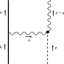
Figure 1: The dotted vertex is the axion-anomaly, $\theta F\widetilde{F}$, and the solid vertical line is the electron. The electron–photon vertex is the magnetic moment of the electron. The incoming axion with 4-momentum $(m_{a},\vec{0})$ absorbs a spacelike photon of 4-momentum $(0,\vec{k})$ with $|\vec{k}|=m_{a}$ to produce an outgoing photon of momentum $\sim(m_{a},\vec{k})$. The electron barely recoils, since $m_{e}>>m_{a}$..

Given the form of this result, we interpret this as an effective, induced OEDM for the electron. We claim this result is general, and the interaction produces electric dipole radiation from any static magnetic moment immersed in, and absorbing energy from, the oscillating cosmic axion field. Indeed, since the result follows from a tree-diagram, it can be demonstrated classically by a straightforward manipulation of Maxwell’s equations, Hill3 . The radiation is formally that of an oscillating (Hertzian) electric dipole, with outgoing electric field polarization aligned in the direction of the magnetic moment, and thus apparently violating CP. The emitted power by a free electron, in a spin-up to spin-up transition, is (for a derivation see section IV.B of Hill2 ):

$$P = \frac{1}{12\pi}(g_{a}\theta_{0}\;\mu_{Bohr})^{2}m^{4}_{a}$$ (2)

This result is equivalent to that obtained from the classical Maxwell equations for a fixed classical magnetic moment $\vec{m}=2\mu_{Bohr}(\vec{s}/2)$ with a spin unit-vector $\vec{s}$ Hill2 ; Hill3 .

More generally, we have computed Fig.(1) in an arbitrary gauge for the background electric field, Hill1 ; Hill2 . We obtained in the static $\vec{P}(x)=\mu_{Bohr}\psi^{\dagger}\vec{\sigma}\psi$ limit:

$$S=g\int d^{4}x\;\theta(t)\left(\vec{P}\cdot\vec{E}+\vec{\nabla}\cdot\vec{P}\left(\frac{1}{\vec{\nabla}^{2}}\right)\vec{\nabla}\cdot\vec{E}\right)$$ (3)

This result differs from the radiation gauge result eq.(1) by the appearance of the nonlocal term. Such nonlocal terms occur in electrodynamics when certain gauge choices are specified, as in the case of the “transverse current,” (see below and Jackson ). Here, $\frac{1}{\vec{\nabla}^{2}}$ is a static Green’s function, i.e.,

$$A(x)\frac{1}{\vec{\nabla}^{2}}B(x)=\int d^{4}y\;A(x)\frac{\delta(x_{0}-y_{0})}{4\pi|\vec{x}-\vec{y}|}B(y)$$ (4)

In an arbitrary gauge, $\vec{E}=\vec{\nabla}\varphi-\partial_{t}\vec{A}$, after integrations by parts, the action of eq.(3) takes the form:

$$S=g\int d^{4}x\;\theta(t)\vec{\nabla}\cdot(\vec{P}\varphi)$$

$$\!\!\!\!\!\!\!\!+g\int d^{4}x\;\partial_{t}\theta(t)\left(\vec{P}\cdot\vec{A}+\vec{\nabla}\cdot\vec{P}\left(\frac{1}{\vec{\nabla}^{2}}\right)\vec{\nabla}\cdot\vec{A}\right)$$ (5)

This result is indeed gauge invariant as can be checked explicitly, as it is just a rewrite of the manifestly gauge invariant eq.(3). If there are no surface terms we can drop the first term on the rhs which is a total divergence, and with $\vec{\nabla}\cdot\vec{A}=0$ (radiation gauge; this follows from $\vec{\nabla}\cdot\vec{E}=0$ upon integrating by parts in time) the result reduces back to eq.(1). It should be noted that the first term on the rhs of eq.(3) or eq.(Reply to “Comment on ‘Axion induced oscillating electric dipole moments’ ”) actually represents a force exerted upon the OEDM by an applied oscillating $\vec{E}$, hence there is potentially more physics here than dipole radiation.

We can now see several flaws with the Flambaum et al. analysis. They have “properly computed” this result in the particular case $\vec{A}=0$ and $A_{0}=\varphi\neq 0$. In this case we see that only the first term will be formally nonzero in eq.(Reply to “Comment on ‘Axion induced oscillating electric dipole moments’ ”), but that term is just a spatial total divergence, and hence it contributes nothing to the physics. A total divergence is zero in momentum space and the Feynman diagram of Fig.(1) then yields zero.

Moreover, Flambaum et al. claim that this is a “gauge choice.” But this is, in fact, a physics choice since one cannot generally make $\vec{A}$ vanish by a gauge transformation. Furthermore, a time dependent $A_{0}=\varphi$ necessarily requires a nonzero $\vec{A}$ by equations of motion as we show in the discussion below eq.(8). Therefore, Flambaum et al. , by using only a Coulomb potential to probe a dynamical time dependent radiating source, are forcing the external field to be static and thus obtain a false null result by Fourier mismatch, as well as total divergence. Finally, their result is consistent with our result in taking the pure Coulomb or static limit, but it is our result which they are attacking!

The many conceptual errors and discrepancies of Flambaum et al. with our results seem to stem from a faulty definition which they claim to be valid for any EDM. They state:

“(1) The EDM of an elementary particle is defined by the linear energy shift that it produces through its interaction with an applied static electric field: $\delta\epsilon=−\vec{d}\cdot\vec{E}$. As we show explicitly, the interaction of an electron with an applied static electric field, in the presence of the axion electromagnetic anomaly, in the lowest order does not produce an energy shift in the limit $v/c\rightarrow 0$. This implies that no electron EDM is generated by this mechanism in the same limit.”

While this definition may be applicable to a static EDM, as in an introductory course in electromagnetism, it is inapplicable to an intrinsically time dependent one. With an OEDM we are dealing with a dynamical situation and must resort to a more general definition, phrased in the context of an action.

We should define the EDM or OEDM of any object as a covariant action of the form:

$$S=g\int d^{4}x\;S_{\mu\nu}(x)F^{\mu\nu}(x)$$ (6)

where $S_{\mu\nu}$ is an antisymmetric odd parity dipole density (e.g., $S_{\mu\nu}\sim\overline{\psi}\sigma_{\mu\nu}\gamma^{5}\psi$ for a relativisitic particle).

For concreteness, let us consider the case of the axion induced neutron OEDM. The neutron OEDM is believed to arise in QCD from instantons. It is being sought in a proposed experiment (see ref.budkher and references therein). In the common rest frame of the neutron and axion, the OEDM action of eq.(6) reduces to:

$$S=g\int d^{4}x\;\theta(t)\vec{P}\cdot\vec{E}(t)$$ (7)

where $\vec{P}(x)=(e/m_{N})\psi^{\dagger}\vec{\sigma}\psi(x)$ is the dipole spin density, written in terms of two-component spinors. $\vec{P}(x)$ is localized in space and static (time independent), and the oscillating aspect of the EDM comes from the axion $\theta(t)$.

Note that a non-recoiling neutron is the kinematically favored limit, e.g., as in Fig.(1). The neutron (or electron) is very heavy compared to the axion, and like a truck being hit by a ping-pong ball can only acquire an insignificant kinetic energy. Therefore, the radiated photon must carry off the full energy of the incident axion, with a 4-momentum of $(m_{a},\vec{k})$, and $|\vec{k}|=m_{a}$ (and the exchange photon 4-momentum is spacelike, $(0,\vec{k})$).

Clearly, for a constant background electric field the actions of eqs.(1,7) average to zero. The radiated photon is necessarily time dependent with frequency $m_{a}$, as will be the case for any OEDM. In the case of a radiation gauge photon, we have $A_{0}=0$ and a non-zero $\vec{A}$ with $\vec{\nabla}\cdot\vec{A}=0$. In this case our action for the neutron OEDM is indistinguishable from the OEDM of the electron of eq.(1). Both require a time dependent $\vec{E}$, and are $\propto\partial_{t}\theta(t)$ upon integration by parts in time.

Our result of eq.(1), induced by the axion-QED anomaly, has also been attacked by several other individuals for violating the Adler decoupling of the axion. The decoupling limit corresponds to $m_{a}\rightarrow 0$ and it superficially appears that eq.(1) does not vanish in this limit as decoupling would dictate (of course, it came from the momentum-space result that was obviously $\propto m_{a}$, and this appears explictly in refHill1 ). However, in refs.Hill2 ; Hill3 the issue of the axion decoupling is studied in detail, and it is found to be somewhat subtle in general.

In fact, eq.(1) displays the same behavior as the anomaly itself. The anomaly, in a constant $\vec{B}$ field, can be written either in a manifestly gauge invariant form $\propto\theta(t)\vec{E}\cdot\vec{B}$ or in a manifestly decoupling form $\propto\partial_{t}(\theta(t))\vec{A}\cdot\vec{B}$ where $\vec{E}=-\partial_{t}\vec{A}$ in a radiation gauge. It is not possible to display simultaneously the manifest decoupling, and gauge invariance. Likewise, in the static electron limit eq.(1) can be written as:

$$\int d^{4}x\;g\;\mu_{Bohr}\partial_{t}{\theta}(t)\psi^{\dagger}\vec{\sigma}\psi\cdot\vec{A}$$ (8)

where $\vec{A}$ is the vector potential. Here we see manifest decoupling, but an expression written in terms of a vector potential. More generally the result in an arbitrary gauge with recoil can be derived and displays the same behavior.

The decoupling is actually subtle and beautiful. One can see this explicitly in the eqs.(56,57) of ref.Hill2 for the near-zone radiation field (and in eqs.(44) for the RF cavity) and in the classical analysis of Hill3 . The decoupling is actually occuring in the spatial structure of the nearzone radiation field (or RF cavity modes). These vanish as $m_{a}^{2}$ due to a “magic cancellation:” the static magnetic dipole field, which multiplies $\theta(t)$, does not radiate and cancels, in the $m_{a}\rightarrow 0$ limit, against the outgoing radiation field which is retarded and proportional to $\theta(t-r/c)$, leaving terms of order $m_{a}^{2}$. This implies that here there is no “Witten effect,” whereby a constant induced electric dipole would remain in the $\theta\rightarrow$ constant limit: the would-be Witten term cancels against the retarded outgoing radiation field in the near-zone. In the end the radiated power is $\propto m_{a}^{4}$, and axion decoupling is certainly working as it should. Such radiation is physically interesting, and may be detectable in experiment Hill2 .

Let us consider the problem of allowing $A_{0}$ to be time dependent while trying to maintain $\vec{A}=0$. $A_{0}$ is a non-propagating field and cannot represent a physical out-going on-shell photon. The equation of motion for $A_{0}$ is $\vec{\nabla}^{2}A_{0}=-\rho(x)$, where $\rho(x)$ is a charge density. If we want to allow time dependent $A_{0}$, then $\nabla^{2}\partial_{0}A_{0}=-\partial_{0}\rho(x,t)$, but from current conservation we have $\partial_{0}\rho(x)=\nabla\cdot\vec{j}$ where $\vec{j}$ is the 3-current. Hence, we have $\partial_{0}A_{0}=-(1/\vec{\nabla}^{2})\vec{\nabla}\cdot\vec{j}$. This means that if $A_{0}$ is to be time dependent, then there must necessarily be a 3-current, hence there is a source for the vector potential, $\vec{A}$, and we cannot maintain $\vec{A}=0$.

Let us impose the condition $\vec{\nabla}\cdot\vec{A}=0$. $\vec{A}$ satisfies $(\partial_{0}^{2}-\nabla^{2})\vec{A}-\vec{\nabla}\partial_{0}A_{0}=\vec{j}$ ( i.e., $\partial_{\mu}F^{\mu i}=j^{i}$ ). This is often written as $(\partial_{0}^{2}-\nabla^{2})\vec{A}=\vec{j}_{T}$ where $\vec{j}_{T}$ is the “transverse current” Jackson . Upon eliminating $\partial_{0}A_{0}$, the transverse current takes the nonlocal form $\vec{j}_{T}=\vec{j}-\vec{\nabla}(1/\nabla^{2})\vec{\nabla}\cdot\vec{j}$. Thus, introducing $A_{0}$ time dependence requires a nonzero vector potential, and its source is essentially nonlocal. The nonlocal term we obtained in eq.(3) is the analogue of the transverse current Hill2 .

As stated above, the calculation in Flambaum, et al. , was restricted to a 4-vector potential of the pure Coulomb form, $A_{\mu}=(A_{0},\vec{0})$ i.e., $\vec{E}=\vec{\nabla}A_{0}$. This is not a gauge choice, since a general 4-vector potential, $A_{\mu}(x,t)$, cannot be brought to the pure timelike form by a gauge transformation, and if $\vec{A}=0$ then $A_{0}$ must be static in time. Thus a pure Coulomb potential cannot probe an OEDM since the action averages to zero in time.

In conclusion, Ref.Flambaum has argued that Fig.(1) is zero. However, they have made specific assumptions that enforce a static electric field configuration, and end up computing a total spatial divergence which is automatically null. From this they argue that there can be no induced effective OEDM for the electron. However, they have not considered the case of a time dependent radiation field, or even a homogeneous field that has a Fourier time component matched to the oscillation frequency of the axion.

The diagram of Fig.(1) represents real physics, and can be interpreted as the effective action of an induced electron OEDM, interacting with a coherent oscillating axion field. It produces electric $N$-pole radiation emanating from any magnetic $N$-pole placed in the oscillating cosmic axion field. This can be seen in various quantum computations at various levels of detail Hill1 ; Hill2 , or directly from Maxwell’s equations Hill3 . The emission of electric dipole radiation from magnets could form a basis for broadband radiative detectors for cosmic axions. These conclusions have certainly not been falsified by the authors of ref.Flambaum .

I thank, for discussions, Bill Bardeen, Aaron Chou, Graham Ross, Arkady Vainshtein, and various members of the Fermilab axion search and breakfast groups. This work was done at Fermilab, operated by Fermi Research Alliance, LLC under Contract No. DE-AC02-07CH11359 with the United States Department of Energy.

References

- (1) C. T. Hill, Phys. Rev. D 91, 111702 (2015)
- (2) C. T. Hill, Phys. Rev. D 93, no. 2, 025007 (2016)
- (3) C. T. Hill, arXiv:1606.04957 .
- (4) V. V. Flambaum, B. M. Roberts and Y. V. Stadnik, preceding comment, Phys. Rev. D 95, no. 5, 058701 (2017)
- (5) J. D. Jackson, Classical Electrodynamics, 2nd ed. (John Wiley and Son’s, 1999), pgs 241-242.
- (6) D. Budker, et al. , Phys. Rev. X 4, no. 2, 021030 (2014)