Minimal physical requirements for crystal growth self-poisoning

Abstract

Self-poisoning is a kinetic trap that can impair or prevent crystal growth in a wide variety of physical settings. Here we use dynamic mean-field theory and computer simulation to argue that poisoning is ubiquitous because its emergence requires only the notion that a molecule can bind in two (or more) ways to a crystal; that those ways are not energetically equivalent; and that the associated binding events occur with sufficiently unequal probability. If these conditions are met then the steady-state growth rate is in general a non-monotonic function of the thermodynamic driving force for crystal growth, which is the characteristic of poisoning. Our results also indicate that relatively small changes of system parameters could be used to induce recovery from poisoning.

I Introduction

One of the kinetic traps that can prevent the crystallization of molecules from solution is the phenomenon of self-posioning, in which molecules attach to a crystal in a manner not commensurate with the crystal structure and so impair or prevent crystal growth Ungar et al. (2005); De Yoreo and Vekilov (2003). This phenomenon has been seen in computer simulations of hard rods Schilling and Frenkel (2004), and in the assembly of polymers Higgs and Ungar (1994); Ungar et al. (2000, 2005) and proteins Asthagiri et al. (2000); Schmit (2013). A signature of self-poisoning is a growth rate that is a non-monotonic function of the thermodynamic driving force for crystal growth, with the slowing of growth as a function of driving force occurring in the rough-growth-front regime (a distinct effect, growth poisoning at low driving force, can occur if impurities impair 2D nucleation on the surface of a 3D crystal Cabrera et al. (1958); Land et al. (1999); Van Enckevort and Van den Berg (1998); Sleutel et al. (2015)). Unlike the slow dynamics associated with nucleation De Yoreo and Vekilov (2003); Sear (2007), self-poisoning cannot be overcome by seeding a solution with a crystal template or by inducing heterogeneous nucleation.

Here we use dynamic mean-field theory and computer simulation to argue that poisoning is ubiquitous because its emergence requires no specific spatial or molecular detail, but only the notion that a molecule can bind in two (or more) ways to a crystal, optimal and non-optimal; that the non-optimal way of binding is energetically less favorable than the optimal way of binding; and that any given binding event is more likely (by about an order of magnitude) to be non-optimal than to be optimal. If these conditions are met then the character of the steady-state growth regime changes qualitatively with crystal-growth driving force. Just past the solubility limit a crystal’s growth rate increases with thermodynamic driving force (supercooling or supersaturation). However, the dynamically-generated crystal also becomes less pure as driving force is increased, i.e. it incorporates more molecules in the non-optimal configuration. As a result, the effective driving force for growth of the impure crystal can diminish as the driving force for growth of the pure crystal increases, and so the impure crystal’s growth slows (this feedback effect is similar to the growth-rate ‘catastrophe’ described in Ref. Van Enckevort and Van den Berg (1998)). At even larger driving forces an impure precipitate of non-optimally-bound molecules grows rapidly. Self-poisoning of polymer crystallization was studied in Refs. Higgs and Ungar (1994); Ungar et al. (2000, 2005) using analytic models and simulations. The present models have a similar minimal flavor to the models developed in those references, although our models are not designed to be models of polymer crystallization specifically, and contain no notion of molecular binding-site blocking. We show that poisoning can happen even if all molecular interactions are attractive, and that it results from a nonlinear dynamical feedback effect that couples crystal quality and crystal growth rate. Having identified the factors that lead to poisoning, the present models also suggest that relatively small changes of system parameters could be used to induce recovery from it.

In Section II we introduce and analyze a mean-field model of the growth of a crystal from molecules able to bind to it in distinct ways. In Section III we introduce a simulation model of the same type of process, but one that accommodates spatial fluctuations and particle-number fluctuations ignored by the mean-field theory. The behavior of these models is summarized in Section IV. Both the mean-field model and the simulations show crystal growth rate to be a non-monotonic function of the thermodynamic driving force for growth of the pure crystal, because the dynamically-generated crystal is in general impure. In some regimes the predictions of the two models differ in their specifics: the mean-field theory assumes a nonequilibrium steady-state of infinite lifetime, and the growth rate associated with this steady-state can vanish. Simulations, which satisfy detailed balance, eventually evolve to thermal equilibrium and so always display a non-zero growth rate. We conclude in Section V.

II Mean-field theory of growth poisoning

The basic physical ingredients of growth poisoning are contained within a model of growth that neglects all spatial detail and accounts only for the ability of particles of distinct type (or, equivalently, distinct conformations of a single particle type) to bind to or unbind from a ‘structure’, which we resolve only in an implicit sense. We consider $K$ types of particle, labeled $i=1,2,\dots,K$ (we will focus shortly on the case of two particle types). We model the structure in a mean-field sense, resolving it only to the extent that we identify the relative abundance $n_{i}$ of particle type $i$ within the structure, where $\sum_{i}n_{i}=1$ (we assume that sums over variables $i$ and $j$ run over all $K$ particle-type labels). Let us assume that the structure gains particles of type $i$ at rate $p_{i}C$, where $C$ is a notional concentration and $\sum_{i}p_{i}=1$. Let us assume that particle types unbind from the structure with a rate proportional to their relative abundance within the structure, multiplied by some rate $\lambda$, which can depend on the set of variables $\{n_{i}\}$. If we write down a master equation for the stochastic process so defined, calculate expectation values of the variables $n_{i}$, and replace fluctuating quantities by their averages, then we get the following set of mean-field rate equations describing the net rates $\Gamma_{i}$ at which particles of type $i$ add to the structure:

$$\Gamma_{i}=p_{i}C-n_{i}\lambda(\{n_{i}\}),$$ (1)

where $i=1,2,\dots,K$, and $\sum_{i}p_{i}=1=\sum_{i}n_{i}$ as stated previously. To model a structure of interacting particles we assume a Boltzmann-like rate of unbinding,

$$\lambda_{i}(\{n_{i}\})=\exp(\beta\sum_{j}\epsilon_{ij}n_{j}),$$ (2)

which assumes the interaction energy between particle types $i$ and $j$ to be $\epsilon_{ij}$, and assumes that particles ‘feel’ only the averaged composition $\{n_{i}\}$ of the structure.

We define the growth rate of the structure as

$$V\equiv\sum_{i}\Gamma_{i}.$$ (3)

In equilibrium the structure neither grows nor shrinks, and we have

$$\Gamma_{i}=0$$ (4)

for each $i=1,2,\dots,K$. We shall also assume the existence of a steady-state growth regime in which $V\geq 0$ but the composition of the structure does not change with time; in this regime we have

$$n_{i}=\frac{\Gamma_{i}}{\sum_{j}\Gamma_{j}},$$ (5)

i.e. the relative abundance of each particle type is proportional to the relative rate at which it is added to the structure.

At this point the set of equations (1) – (5) describes a generic model of growth via the binding and unbinding of particles of multiple types. The model is mean-field in both a spatial sense – no spatial degrees of freedom exist, and particle-structure interactions depend on the composition of the structure as a whole – and in the sense of ignoring fluctuations of particle number: the model resolves only net rates of growth. We now specialize the model to the case of crystal growth in the presence of impurities; different choices of parameters can be used to model other scenarios Whitelam et al. (2014); Sue et al. (2015); Mannige and Whitelam (2015).

We shall consider two particle types, and so set $K=2$. We will call particle types 1 and 2 ‘B’ for ‘blue’ and ‘R’ for ‘red’, respectively, for descriptive purposes (in Section IV simulation configurations will be color-coded accordingly). We call the relative abundance of blue particles in the structure $n_{1}\equiv n$, and so the relative abundance of red particles in the structure is $n_{2}=1-n$. We consider blue particles to represent the (unique) crystallographic orientation and conformation of a particular molecule, and red particles to represent the ensemble of non-crystallographic orientations and conformations of the same molecule. Alternatively, one could consider red particles to be an impurity species present in the same solution as the blue particles that we want to crystallize. We assume that an isolated particle is blue with probability $p$ and red with probability $1-p$, and so we choose $p_{1}=p$ and so $p_{2}=1-p$ for the basic rates of particle addition in (1). We will assume that the blue-blue crystallographic or ‘specific’ interaction in Eq. (2) is $\epsilon_{\rm BB}=-\epsilon_{\rm s}k_{\rm B}T$. We will assume that interactions between blue and red ($\epsilon_{\rm RB}$) or red and red ($\epsilon_{\rm RR}$) are ‘nonspecific’, and equal to $-\epsilon_{\rm n}k_{\rm B}T$. With these choices (1) reads

$$\Gamma_{\rm B} = pC-n\alpha^{n}{\rm e}^{-\epsilon_{\rm n}},$$ (6)

$$\Gamma_{\rm R} = (1-p)C-(1-n){\rm e}^{-\epsilon_{\rm n}},$$ (7)

where $\alpha\equiv{\rm e}^{-\Delta}$ and $\Delta\equiv\epsilon_{\rm s}-\epsilon_{\rm n}$. This model describes the growth of a structure whose character is defined by its ‘color’, $n$; for $n\approx 1$ the structure is almost blue, and we shall refer to this structure as the ‘crystal’. For $n$ small we have a mostly red structure, and we refer to this as the ‘precipitate’. Intermediate values of $n$ describe a structure that we shall refer to as an ‘impure’ crystal.

It is convenient to work with a set of rescaled rates and concentrations

$$\left(c,\gamma_{\rm R},\gamma_{\rm B}\right)\equiv\left(C,\Gamma_{\rm R},\Gamma_{\rm B}\right){\rm e}^{\epsilon_{\rm n}},$$ (8)

in terms of which Equations (6) and (7) read

$$\gamma_{\rm B} = pc-n\alpha^{n}.$$ (9)

$$\gamma_{\rm R} = (1-p)c-(1-n).$$ (10)

The rescaling defined by Eq. (8) makes an important physical point: the timescale for crystal growth is measured most naturally in terms of the basic timescale ${\rm e}^{\epsilon_{\rm n}}$ for the unbinding of impurity (red) particles. Thus, for fixed energy scale $\epsilon_{\rm n}k_{\rm B}T$, lowering temperature serves to increase this basic timescale, indicating that cooling is not necessarily a viable strategy for speeding crystal growth.

Equation (5), which reduces to

$$\frac{n}{1-n}=\frac{\gamma_{\rm B}}{\gamma_{\rm R}},$$ (11)

is the assumption that there exists a steady-state dynamic regime in which the relative abundance of red and blue particles in the growing structure is equal to the ratio of their rates of growth. Inserting into this condition Equations (9) and (10) gives the self-consistent relation

$$\frac{n}{1-n}=\frac{pc-n\alpha^{n}}{(1-p)c-(1-n)}.$$ (12)

One can solve this equation graphically for solid composition $n$, as a function of the parameters $\epsilon_{\rm s},\epsilon_{\rm n},c$, and $p$. To determine the growth rate of the solid one inserts the value of $n$ so calculated into Equations (9) and (10), and adds them:

$$v=\gamma_{\rm R}+\gamma_{\rm B}.$$ (13)

The physical growth rate is then $V=v{\rm e}^{-\epsilon_{\rm n}}$, obtained by undoing the rescaling (8).

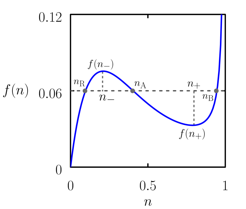
Figure 1: Graphical construction used to determine the phase diagram of the mean-field model of growth poisoning (see Fig. 2(a)). The solutions of Eq. (17) give the solid compositions at which the growth rate vanishes. The horizontal dotted line shows a value of $p/(1-p)$ for which three such solutions exist; the associated values $n_{\rm B}$, $n_{\rm A}$ and $n_{\rm R}$ lie on the ‘solubility’, ‘arrest’, and ‘precipitation’ lines shown in Fig. 2(a).

To gain insight into the behavior of the model is it useful to solve Eq. (12) for $c$,

$$c=\frac{n(1-n)}{n-p}\left(1-\alpha^{n}\right),$$ (14)

and to use this expression to eliminate $c$ from (13), giving

$$v=\frac{1}{n-p}\left[(1-n)p-n(1-p)\alpha^{n}\right].$$ (15)

Equations (14) and (15) can be regarded as parametric equations for the concentration $c$ at which one observes a particular growth rate $v$ of a solid of composition $n$ . Note that $v$ can be negative for certain parameter combinations, indicating a breakdown of the assumption of a steady-state growth regime. The basic phenomenology revealed by Equations (14) and (15) is that altering concentration $c$ results in a change of composition $n$ of the growing structure, and that changes of both $c$ and $n$ affect the rate of growth $v$.

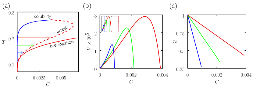
Figure 2: Dynamic mean-field theory predicts that crystal growth rate is a non-monotonic function of concentration. (a) Mean-field phase diagram in the temperature $(T)$-concentration $(C)$ plane derived from Equations (17) and (22). The line marked ‘solubility’ shows the concentration at which the crystal (the ‘blue’ solid) neither grows nor shrinks; the line marked ‘precipitation’ is the same thing for the impure (‘red’) precipitate. The line marked ‘arrest’ shows where the growth rate of the (impure) crystal goes to zero. (b) Growth rate $V$ and (c) crystal quality $n$ as a function of concentration at the three temperatures indicated in the left panel (line colors correspond to arrow colors), obtained from Equations (12) and (13). At the solubility line the crystal does not grow; upon supersaturation it grows with finite speed $V$ and becomes less pure. Consequently, its growth rate begins to decline for sufficiently large $C$, going to zero at the arrest line. Beyond the precipitation line the precipitate grows rapidly (see inset in (b), drawn as in the main panel but with $C$ extended to just beyond the precipitation line). Parameters: $p=10^{-2}$; $\Delta/T\equiv(\epsilon_{\rm s}-\epsilon_{\rm n})/T=2/T$; $\epsilon_{\rm n}/T=1/T$.

In certain parameter regimes $v$ can become a non-monotonic function of $c$, which is crystal growth poisoning. This potential can be seen from (15); setting $\partial v/\partial n=0$ yields 

$$p=\frac{n^{2}\Delta}{{\rm e}^{n\Delta}-1+n\Delta}.$$ (16)

The right-hand side of this equation is a non-monotonic function of $n$, and takes its maximum value when $n=2/\Delta$. Thus for $\Delta>2$ this equation has two solutions (equivalent to turning points of $v(n)$) provided that $\Delta(e^{\Delta}-1+\Delta)^{-1}<p<4\Delta^{-1}(1+{\rm e}^{2})^{-1}$. These two solutions underpin the behavior shown in Fig. 2: increasing concentration first causes the structure to grow more rapidly (because we increase the driving force for crystal growth), and then more slowly (as poisoning happens), and then more quickly again (as the structure grows in an ‘impure’ way). For $\Delta=4$ (see below) poisoning happens if $p<(1+{\rm e}^{2})^{-1}\approx 0.12$. That is, for poisoning to happen the impure (red) species must be at least about 10 times more abundant in solution than the crystal-forming (blue) species.

Of particular interest are the locations in phase space where the growth rate vanishes. These locations can be identified by setting the right-hand side of (15) to zero (or equivalently setting $\gamma_{\rm B}=\gamma_{\rm R}=0$ in Equations (9) and (10)), giving

$$\frac{p}{1-p}=f(n)$$ (17)

where

$$f(n)=\frac{n}{1-n}\alpha^{n}.$$ (18)

Recall that $\alpha\equiv{\rm e}^{-\Delta}$ and $\Delta\equiv\epsilon_{\rm s}-\epsilon_{\rm n}$. Inspection of the properties of $f(n)$ reveals the conditions under which growth arrest can occur. To this end it is convenient to calculate the stationary points $n_{\pm}$ of $f(n)$, which are

$$n_{\pm}=\frac{1}{2}\left(1\pm\sqrt{1-4\Delta^{-1}}\right).$$ (19)

Two stationary points exist for $\Delta>4$, where the function $f(n)$ has the behavior shown in Fig. 1. Arrest can happen if the horizontal line $p/(1-p)$ lies between the values $f(n_{-})$ and $f(n_{+})$, i.e. if

$$\frac{f(n_{-})}{1+f(n_{-})}>p>\frac{f(n_{+})}{1+f(n_{+})},$$ (20)

where

$$f(n_{\pm})=\frac{1\pm\chi}{1\mp\chi}\exp\left\{-\frac{\Delta}{2}\left(1\pm\chi\right)\right\},$$ (21)

with $\chi\equiv\sqrt{1-4\Delta^{-1}}$. In this case there are three solutions $n_{\theta}$ to Eq. (17). We shall call these solutions $n_{\rm B}$, $n_{\rm A}$, and $n_{\rm R}$. From Eq. (10) the associated concentrations $c_{\theta}$ are

$$c_{\theta}=\frac{1-n_{\theta}}{1-p},$$ (22)

where $\theta=$ R, B, or A. The solution corresponding to the largest value of $n$ we call $n_{\rm B}$ (B for blue). The associated concentration $c_{\rm B}$ is that at which the mostly-blue solid or ‘crystal’ is in equilibrium, and we shall call the locus of such values, calculated for different parameter combinations, the ‘solubility line’. The solution corresponding to the smallest value of $n$ we call $n_{\rm R}$ (R for red). The associated concentration is that at which the mostly-red ‘precipitate’ is in equilibrium, and this lies on what we will call the ‘precipitation line’. The remaining solution we call $n_{\rm A}$ (A for arrest); it yields the concentration at which the impure crystal ceases to grow, and it lies on the ‘arrest line’.

Arrest therefore occurs when $\Delta$ is large enough that the (blue) crystal is stable thermodynamically and $p$ is small enough that the crystal’s emergence is kinetically hindered. If $p$ is large enough, i.e. if $p/(1-p)$ is greater than $f(n_{-})$, then the crystal’s emergence is not kinetically hindered and growth arrest does not occur. Conversely, if $p$ is too small, i.e. if $p/(1-p)$ is less than $f(n_{+})$, then $\Delta$ is too small to render the crystal thermodynamically stable.

We can use this set of equations to determine the behavior of our mean-field model of crystal growth, and we describe this behavior in Section IV. There we revert to ‘physical’ growth rates $V$ and concentrations $C$; these are related to their rescaled counterparts $v$ and $c$ via Eq. (8).

III Computer simulations of two-component growth

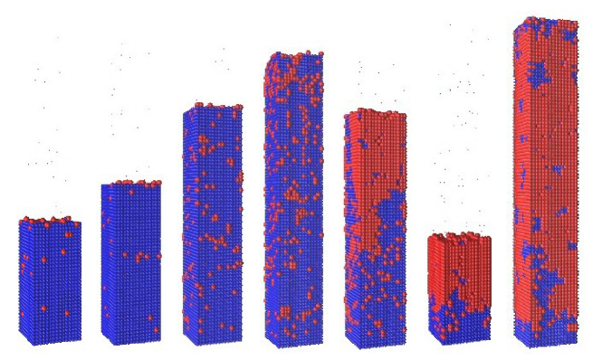
Figure 3: Simulation snapshots taken after fixed long times ($5\times 10^{9}$ MC sweeps) for a range of concentrations $c$ (increasing from left to right) bear out the key prediction of mean-field theory: growth rate is a non-monotonic function of the driving force for crystal growth. Growth rate first increases and then decreases with concentration, because the growing structure becomes less pure (more red). The right-hand snapshot lies beyond the precipitation line, where the impure solid grows rapidly. Parameters: $p=10^{-2}$; $\epsilon_{\rm s}=3.5$; $\epsilon_{\rm n}=1.4$. From left to right, values of $c$ are $0.008,0.0083,0.009875,0.0119,0.014225,0.0149,0.01512$.

We carried out lattice Monte Carlo simulations of two-component growth, similar to those done in Refs. Whitelam et al. (2014); Hedges et al. (2014); Sue et al. (2015); Mannige and Whitelam (2015). Simulations, which satisfy detailed balance with respect to a particular lattice energy function, accommodate spatial degrees of freedom and particle-number fluctuations omitted by the mean-field theory. Simulations therefore provide an assessment of which physics is captured by the mean-field theory and which it omits.

Simulation boxes consisted of a 3D cubic lattice of $15\times 15\times 100$ sites. Sites can be vacant (white), or occupied by a blue particle or a red particle. Periodic boundary conditions were applied along the two short directions. At each time step a site was chosen at random. If the chosen site was white then we proposed with probability $p$ to make it blue, and with probability $1-p$ to make it red. If the chosen site was red or blue then we proposed to make it white. No red-blue interchange was allowed. To model the slow dynamics in the interior of an aggregate we allowed no changes of state of any lattice site that had 6 colored nearest neighbors.

These proposals we accepted with the following probabilities:

$$\textrm{R}\to\textrm{W} : \min\left(1,(1-p){\rm e}^{-\beta\Delta E}\right);$$

$$\textrm{W}\to\textrm{R} : \min\left(1,(1-p)^{-1}{\rm e}^{-\beta\Delta E}\right);$$

$$\textrm{B}\to\textrm{W} : \min\left(1,p\,{\rm e}^{-\beta\Delta E}\right);$$

$$\textrm{W}\to\textrm{B} : \min\left(1,p^{-1}{\rm e}^{-\beta\Delta E}\right),$$

where $\Delta E$ is the energy change resulting from the proposed move. This change was calculated from the lattice energy function

$$E=\sum_{<i,j>}\epsilon_{C(i)C(j)}+\sum_{i}\mu_{C(i)}.$$ (23)

The first sum runs over all distinct nearest-neighbor interactions and the second sum runs over all sites. The index $C(i)$ describes the color of site $i$, and is W (white), B (blue) or R (red); $\epsilon_{C(i)C(j)}$ is the interaction energy between colors $C(i)$ and $C(j)$; and the chemical potential $\mu_{C(i)}$ is $\mu k_{\rm B}T$, $-k_{\rm B}T\ln p$ and $-k_{\rm B}T\ln(1-p)$ for W, B and R, respectively (note that positive $\mu$ favors particles over vacancies). In keeping with the choices made in Section II we take

$$\epsilon_{\rm BB}=-\epsilon_{\rm s}k_{\rm B}T;$$ (24)

$$\epsilon_{\rm BR}=\epsilon_{\rm RB}=\epsilon_{\rm RR}=-\epsilon_{\rm n}k_{\rm B}T.$$ (25)

In the absence of pairwise energetic interactions the likelihood that a given site will be white, blue or red is respectively $1/(1+{\rm e}^{\mu})$, $p/(1+{\rm e}^{-\mu})$, and $(1-p)/(1+{\rm e}^{-\mu})$.

Simulations were begun with three complete layers of blue particles at one end of the box to eliminate the need for spontaneous nucleation. For fixed values of energetic parameters we measured the composition $n$ (the fraction of colored blocks that are blue) and growth rate of the structure produced at different values of the parameter $c\equiv{\rm e}^{\mu}$ (which for small $c$ is approximately equal to the likelihood than an isolated site will in equilibrium be colored rather than white).

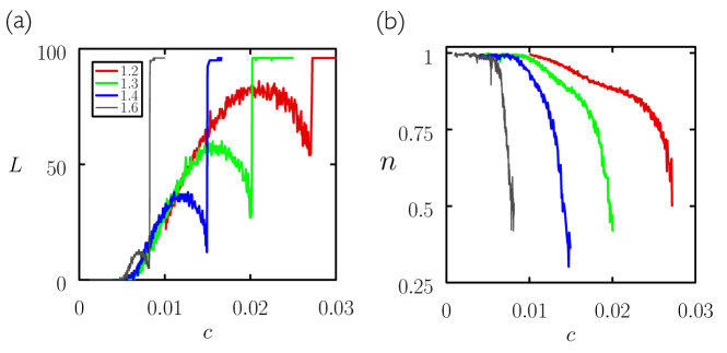
Figure 4: Simulations show a non-monotonic growth rate and decline of crystal quality as the driving force for crystal growth is increased. Number of deposited layers $L$ (a) and crystal quality $n$ (b) after $5\times 10^{9}$ MC sweeps as a function of concentration $c$, for simulations run at various values of the nonspecific interaction parameter $\epsilon_{\rm n}$ (plot legends show values of $\epsilon_{\rm n}$). The spike in growth rate at large $c$ signals the passing of the precipitation line. Other parameters: $p=10^{-2}$; $\epsilon_{\rm s}=3.5$.

IV Results

Fig. 2(a) shows the phase diagram of our mean-field model of crystal growth. The ‘solubility’ and ‘precipitation’ lines indicate where the crystal and precipitate are in equilibrium; the ‘arrest’ line shows where the growth rate of the impure crystal vanishes. The structure of this diagram is similar to that of certain experimental systems – see e.g. Refs. Asherie (2004); Luft et al. (2011a) or Fig. 14 of Ref. Ungar et al. (2005) – showing that the mean-field theory, although simple, can capture important features of real systems. Upon moving left to right across this diagram we observe the behavior shown in panels (b) and (c) of the figure. Growth rate $V$ first increases with concentration $C$, because the thermodynamic driving force for crystal growth increases. But at some point $V$ begins to decrease, i.e. poisoning occurs. This is so because the composition of the growing solid changes with concentration – it becomes less pure – and so the thermodynamic driving force for its growth decreases, even through the thermodynamic driving force for the growth of the pure crystal increases with $C$. As we pass the precipitation line the growth rate $V$ becomes large and positive (inset to panel (b)). This behavior is similar to that seen in e.g. Fig. 2 of Ref. Ungar et al. (2000).

The mean-field theory is simple in nature but furnishes non-trivial predictions. Key aspects of these predictions are borne out by our simulations, which resolve spatial detail and particle-number fluctuations omitted by the theory (we found similar theory-simulation correspondence in a different regime of parameter space Whitelam et al. (2014)). In Fig. 3 we show simulation snapshots, taken after fixed long times, for a range of values of concentration $c$. One can infer from this picture that growth rate is a non-monotonic function of concentration. In all cases the equilibrium structure is a box mostly filled with blue particles. At small concentrations we see the growth of a structure similar to the equilibrium one. Poisoning occurs because the grown structure becomes less pure (more red) as $c$ increases, and so the effective driving force for its growth decreases even though the driving force for the growth of the pure crystal increases. At large concentrations we pass the precipitation line and the impure (red) solid grows rapidly.

In Fig. 4 we show the number of layers $L$ deposited after fixed long simulation times for various concentrations $c$ (we consider a layer to have been added if more than half the sites in a given slice across the long box direction are are occupied by red or blue particles). The general trend seen in simulations is similar to that seen in the mean-field theory (panels (b) and (c) of Fig. 2). At concentrations just above the blue solubility limit the structure’s growth rate increases approximately linearly with concentration. At higher concentrations the growth rate reaches a maximum and then drops sharply, because structure quality (and so the effective driving force for its growth) declines with concentration. One difference between mean-field theory and simulations is that in the latter the growth rate in the poisoning regime does not go to zero. This is so because simulations satisfy detailed balance, and must eventually evolve to equilibrium. Fluctuations (mediated within the bulk of the structure by vacancies) allow the composition of an arrested structure to evolve slowly toward equilibrium, and thereby to extend slowly. Thus the steady-state dynamic regime that has infinite lifetime with the mean-field theory has only finite lifetime within our simulations (because these eventually must reach equilibrium). Slow evolution of this nature is shown in Fig. 5.

Figure 5: Simulations satisfy detailed balance and so eventually evolve to equilibrium. Here we show a time-ordered series of snapshots from a simulation done within the precipitation regime. Fluctuations allow the eventual emergence of the thermodynamically stable crystal structure. Parameters: $p=10^{-2}$; $\epsilon_{\rm s}=3.5$; $\epsilon_{\rm n}=1.2$; $c=0.0274$.

V Conclusions

We have used mean-field theory and computer simulation to show that crystal growth self-poisoning requires no particular spatial or molecular detail, as long as a small handful of physical ingredients are realized. These ingredients are: the notion that a molecule can bind in two (or more) ways to a crystal; that those ways are not energetically equivalent; and that they are realized with sufficiently unequal probability. If these conditions are met then the steady-state growth rate of a structure is, in general, a non-monotonic function of the thermodynamic driving force for crystal growth. Self-poisoning is seen in a wide variety of physical systems Schilling and Frenkel (2004); Ungar et al. (2005); Asthagiri et al. (2000), because, we suggest, many molecular systems display the three physical ingredients we have identified as being sufficient conditions for poisoning. Protein crystallization, for instance, is notoriously difficult, and rational guidance for it is much needed ten Wolde and Frenkel (1997); George and Wilson (1994); Shim et al. (2007); Haxton and Whitelam (2012); Schmit and Dill (2012); Fusco and Charbonneau (2015). The present model suggests that proteins are prime candidates for self-poisoning because they have smaller effective values of the $p$ parameter (which controls the relative rates of binding of optimal and non-optimal contacts) than do relatively rigid small molecules: proteins are anisotropic, conformationally flexible objects whose non-crystallographic modes of binding outnumber their crystallographic mode of binding by a factor of order $10^{4}$ or $10^{5}$ Kierzek et al. (1997); Asthagiri et al. (2000); Schmit and Dill (2012). Many protein crystallization trials result in clear solutions without any obvious indication of why crystals failed to appear Luft et al. (2011b), and in some of these cases self-poisoning might be happening. In general terms decreasing $p$ leaves a system vulnerable to poisoning because a) the rate of attachment of non-crystallographic conformations increases, and b) to ensure thermodynamic stability of the crystal one must increase the basic binding energy scale, in which case the basic timescale for growth increases.

There also exists a possible connection between the present work and the recent observation of protein clusters that appear in weakly-saturated solution and do not grow or shrink Pan et al. (2010). Other authors have proposed Pan et al. (2010) and formulated Lutsko and Nicolis (2015) models that explain the long-lived nature of such clusters via the slow interconversion of oligomeric and monomeric protein: in these models there exists a thermodynamic driving force to grow clusters of oligomers, but the growth of such clusters is hindered by the existence of monomeric protein. If we reinterpret the present model to regard the ‘red’ species as monomeric protein and the ‘blue’ species as oligomeric protein, then we obtain a possible connection to the mechanism described in Refs. Pan et al. (2010); Lutsko and Nicolis (2015). From e.g. Fig. 2(a) we see that we can be in a region of phase space that is undersaturated with respect to monomeric (red) protein but supersaturated with respect to oligomeric (blue) protein (i.e. the thermodynamic ground state is a condensed structure built from oligomeric protein). There then exists a thermodynamic driving force to grow structures made of oligomeric protein, but the emergence of such structures is rendered slow by kinetic trapping (caused by the fact that monomeric protein is more abundant in isolation than is oligomeric protein). According to this interpretation the ‘stable’ protein clusters are kinetically trapped, and on long enough timescales would grow. However, we stress that this connection is tentative.

Having identified factors that lead to poisoning, the present models also suggest that relatively small changes of system parameters could be used to avoid it. For instance, Fig. 2 and Fig. 4 show that, given a set of molecular characteristics, small changes of concentration or temperature can take one from a poisoned regime to one in which crystal growth rate is relatively rapid. Recovery from poisoning could also be effected if one has some way of altering molecular characteristics, such as the value of the non-optimal binding energy scale; see Fig. 4 and Fig. 6.

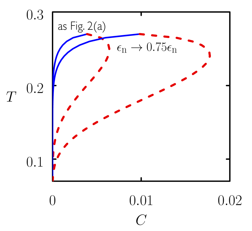
Figure 6: Solubility and arrest line calculated from mean-field theory as in Fig. 2 (with no precipitation line drawn), with a second solution, the larger loop to the right, drawn for the case of diminished nonspecific binding energy $\epsilon_{\rm n}\to 3\epsilon_{\rm n}/4$ (with $\Delta$ unchanged). This change greatly enlarges the region of phase space in which crystal growth can happen.