Abstract

There are various parametric models for analyzing pairwise comparison data, including the Bradley-Terry-Luce (BTL) and Thurstone models, but their reliance on strong parametric assumptions is limiting. In this work, we study a flexible model for pairwise comparisons, under which the probabilities of outcomes are required only to satisfy a natural form of stochastic transitivity. This class includes parametric models including the BTL and Thurstone models as special cases, but is considerably more general. We provide various examples of models in this broader stochastically transitive class for which classical parametric models provide poor fits. Despite this greater flexibility, we show that the matrix of probabilities can be estimated at the same rate as in standard parametric models. On the other hand, unlike in the BTL and Thurstone models, computing the minimax-optimal estimator in the stochastically transitive model is non-trivial, and we explore various computationally tractable alternatives. We show that a simple singular value thresholding algorithm is statistically consistent but does not achieve the minimax rate. We then propose and study algorithms that achieve the minimax rate over interesting sub-classes of the full stochastically transitive class. We complement our theoretical results with thorough numerical simulations.

1 Introduction

Pairwise comparison data is ubiquitous and arises naturally in a variety of applications, including tournament play, voting, online search rankings, and advertisement placement problems. In rough terms, given a set of $n$ objects along with a collection of possibly inconsistent comparisons between pairs of these objects, the goal is to aggregate these comparisons in order to estimate underlying properties of the population. One property of interest is the underlying matrix of pairwise comparison probabilities—that is, the matrix in which entry $(i,j)$ corresponds to the probability that object $i$ is preferred to object $j$ in a pairwise comparison. The Bradley-Terry-Luce [BT52, Luc59] and Thurstone [Thu27] models are mainstays in analyzing this type of pairwise comparison data. These models are parametric in nature: more specifically, they assume the existence of an $n$-dimensional weight vector that measures the quality or strength of each item. The pairwise comparison probabilities are then determined via some fixed function of the qualities of the pair of objects. Estimation in these models reduces to estimating the underlying weight vector, and a large body of prior work has focused on these models (e.g., see the papers [NOS12, HOX14, SBB⁺16]). However, such models enforce strong relationships on the pairwise comparison probabilities that often fail to hold in real applications. Various papers [DM59, ML65, Tve72, BW97] have provided experimental results in which these parametric modeling assumptions fail to hold.

Our focus in this paper is on models that have their roots in social science and psychology (e.g., see Fishburn [Fis73] for an overview), in which the only coherence assumption imposed on the pairwise comparison probabilities is that of strong stochastic transitivity, or SST for short. These models include the parametric models as special cases but are considerably more general. The SST model has been validated by several empirical analyses, including those in a long line of work [DM59, ML65, Tve72, BW97]. The conclusion of Ballinger et al. [BW97] is especially strongly worded:

All of these parametric c.d.f.s are soundly rejected by our data. However, SST usually survives scrutiny.

We are thus provided with strong empirical motivation for studying the fundamental properties of pairwise comparison probabilities satisfying SST.

In this paper, we focus on the problem of estimating the matrix of pairwise comparison probabilities—that is, the probability that an item $i$ will beat a second item $j$ in any given comparison. Estimates of these comparison probabilities are useful in various applications. For instance, when the items correspond to players or teams in a sport, the predicted odds of one team beating the other are central to betting and bookmaking operations. In a supermarket or an ad display, an accurate estimate of the probability of a customer preferring one item over another, along with the respective profits for each item, can effectively guide the choice of which product to display. Accurate estimates of the pairwise comparison probabilities can also be used to infer partial or full rankings of the underlying items.

Our contributions:

We begin by studying the performance of optimal methods for estimating matrices in the SST class: our first main result (Theorem 1) characterizes the minimax rate in squared Frobenius norm up to logarithmic factors. This result reveals that even though the SST class of matrices is considerably larger than the classical parametric class, surprisingly, it is possible to estimate any SST matrix at nearly the same rate as the classical parametric family. On the other hand, our achievability result is based on an estimator involving prohibitive computation, as a brute force approach entails an exhaustive search over permutations. Accordingly, we turn to studying computationally tractable estimation procedures. Our second main result (Theorem 2) applies to a polynomial-time estimator based on soft-thresholding the singular values of the data matrix. An estimator based on hard-thresholding was studied previously in this context by Chatterjee [Cha14]. We sharpen and generalize this previous analysis, and give a tight characterization of the rate achieved by both hard and soft-thresholding estimators. Our third contribution, formalized in Theorems 3 and 4, is to show how for certain interesting subsets of the full SST class, a combination of parametric maximum likelihood [SBB⁺16] and noisy sorting algorithms [BM08] leads to a tractable two-stage method that achieves the minimax rate. Our fourth contribution is to supplement our minimax lower bound with lower bounds for various known estimators, including those based on thresholding singular values [Cha14], noisy sorting [BM08], as well as parametric estimators [NOS12, HOX14, SBB⁺16]. These lower bounds show that none of these tractable estimators achieve the minimax rate uniformly over the entire class. The lower bounds also show that the minimax rates for any of these subclasses is no better than the full SST class.

Related work:

The literature on ranking and estimation from pairwise comparisons is vast and we refer the reader to various surveys [FV93, Mar96, Cat12] for a more detailed overview. Here we focus our literature review on those papers that are most closely related to our contributions. Some recent work [NOS12, HOX14, SBB⁺16] studies procedures and minimax rates for estimating the latent quality vector that underlie parametric models. Theorem 4 in this paper provides an extension of these results, in particular by showing that an optimal estimate of the latent quality vector can be used to construct an optimal estimate of the pairwise comparison probabilities. Chatterjee [Cha14] analyzed matrix estimation based on singular value thresholding, and obtained results for the class of SST matrices. In Theorem 2, we provide a sharper analysis of this estimator, and show that our upper bound is—in fact—unimprovable.

In past work, various authors [KMS07, BM08] have considered the noisy sorting problem, in which the goal is to infer the underlying order under a so-called high signal-to-noise ratio (SNR) condition. The high SNR condition means that each pairwise comparison has a probability of agreeing with the underlying order that is bounded away from ${\frac{1}{2}}$ by a fixed constant. Under this high SNR condition, these authors provide polynomial-time algorithms that, with high probability, return an estimate of true underlying order with a prescribed accuracy. Part of our analysis leverages an algorithm from the paper [BM08]; in particular, we extend their analysis in order to provide guarantees for estimating pairwise comparison probabilities as opposed to estimating the underlying order.

As will be clarified in the sequel, the assumption of strong stochastic transitivity has close connections to the statistical literature on shape constrained inference (e.g., [SS11]), particularly to the problem of bivariate isotonic regression. In our analysis of the least-squares estimator, we leverage metric entropy bounds from past work in this area (e.g., [GW07, CGS15]).

In Appendix D of the present paper, we study estimation under two popular models that are closely related to the SST class, and make even weaker assumptions. We show that under these moderate stochastic transitivity (MST) and weak stochastic transitivity (WST) models, the Frobenius norm error of any estimator, measured in a uniform sense over the class, must be almost as bad as that incurred by making no assumptions whatsoever. Consequently, from a statistical point of view, these assumptions are not strong enough to yield reductions in estimation error. We note that the “low noise model” studied in the paper [RA14] is identical to the WST class.

Organization:

The remainder of the paper is organized as follows. We begin by providing a background and a formal description of the problem in Section 2. In Section 3, we present the main theoretical results of the paper. We then present results from numerical simulations in Section 4. We present proofs of our main results in Section 5. We conclude the paper in Section 6.

2 Background and problem formulation

Given a collection of $n\geq 2$ items, suppose that we have access to noisy comparisons between any pair $i\neq j$ of distinct items. The full set of all possible pairwise comparisons can be described by a probability matrix $M^{*}\in[0,1]^{n\times n}$, in which $M^{*}_{ij}$ is the probability that item $i$ is preferred to item $j$. The upper and lower halves of the probability matrix $M^{*}$ are related by the shifted-skew-symmetry condition $M^{*}_{ji}=1-M^{*}_{ij}$ for all $i,j\in[n]$. For concreteness, we set $M^{*}_{ii}=1/2$ for all $i\in[n]$.

2.1 Estimation of pairwise comparison probabilities

For any matrix $M^{*}\in[0,1]^{n\times n}$ with $M^{*}_{ij}=1-M^{*}_{ji}$ for every $(i,j)$, suppose that we observe a random matrix $Y\in\{0,1\}^{n\times n}$ with (upper-triangular) independent Bernoulli entries, in particular, with $\mathbb{P}[Y_{ij}=1]=M^{*}_{ij}$ for every $1\leq i\leq j\leq n$ and $Y_{ji}=1-Y_{ij}$. Based on observing $Y$, our goal in this paper is to recover an accurate estimate, in the squared Frobenius norm, of the full matrix $M^{*}$.

Our primary focus in this paper will be on the setting where for $n$ items we observe the outcome of a single pairwise comparison for each pair. We will subsequently (in Section 3.5) also address the more general case when we have partial observations, that is, when each pairwise comparison is observed with a fixed probability.

For future reference, note that we can always write the Bernoulli observation model in the linear form

$$Y =M^{*}+W,$$ (1)

where $W\in[-1,1]^{n\times n}$ is a random matrix with independent zero-mean entries for every $i\geq j$ given by

$$W_{ij} \sim\begin{cases}1-M^{*}_{ij}&\mbox{with probability $M^{*}_{ij}$}\\ -M^{*}_{ij}&\mbox{with probability $1-M^{*}_{ij}$,}\end{cases}$$ (2)

and $W_{ji}=-W_{ij}$ for every $i<j$. This linearized form of the observation model is convenient for subsequent analysis.

2.2 Strong stochastic transitivity

Beyond the previously mentioned constraints on the matrix $M^{*}$—namely that $M^{*}_{ij}\in[0,1]$ and $M^{*}_{ij}=1-M^{*}_{ij}$—more structured and interesting models are obtained by imposing further restrictions on the entries of $M^{*}$. We now turn to one such condition, known as strong stochastic transitivity (SST), which reflects the natural transitivity of any complete ordering. Formally, suppose that the full collection of items $[n]$ is endowed with a complete ordering $\pi^{*}$. We use the notation $\pi^{*}(i)<\pi^{*}(j)$ to convey that item $i$ is preferred to item $j$ in the total ordering $\pi^{*}$. Consider some triple $(i,j,k)$ such that $\pi^{*}(i)<\pi^{*}(j)$. A matrix $M^{*}$ satisfies the SST condition if the inequality $M^{*}_{ik}\geq M^{*}_{jk}$ holds for every such triple. The intuition underlying this constraint is the following: since $i$ dominates $j$ in the true underlying order, when we make noisy comparisons, the probability that $i$ is preferred to $k$ should be at least as large as the probability that $j$ is preferred to $k$. The SST condition was first described in the psychology literature (e.g., [Fis73, DM59]).

The SST condition is characterized by the existence of a permutation such that the permuted matrix has entries that increase across rows and decrease down columns. More precisely, for a given permutation $\pi^{*}$, let us say that a matrix $M$ is $\pi^{*}$-faithful if for every pair $(i,j)$ such that $\pi^{*}(i)<\pi^{*}(j)$, we have $M_{ik}\geq M_{jk}$ for all $k\in[n]$. With this notion, the set of SST matrices is given by

$$\mathbb{C}_{\mbox{\scalebox{0.5}{{SST}}}}=\big{\{}M\in[0,1]^{n\times n}\,\mid\, \mbox{ $M_{ba}=1-M_{ab}\;\forall\;(a,b)$, and $\exists$ perm. $\pi^{*}$ s.t. $M$ is $\pi^{*}$-faithful}\big{\}}.$$ (3)

Note that the stated inequalities also guarantee that for any pair with $\pi^{*}(i)<\pi^{*}(j)$, we have $M_{ki}\leq M_{kj}$ for all $k$, which corresponds to a form of column ordering. The class $\mathbb{C}_{\mbox{\scalebox{0.5}{{SST}}}}$ is our primary focus in this paper.

2.3 Classical parametric models

Let us now describe a family of classical parametric models, one which includes Bradley-Terry-Luce and Thurstone (Case V) models [BT52, Luc59, Thu27]. In the sequel, we show that these parametric models induce a relatively small subclass of the SST matrices $\mathbb{C}_{\mbox{\scalebox{0.5}{{SST}}}}$.

In more detail, parametric models are described by a weight vector $w^{*}\in\mathbb{R}^{n}$ that corresponds to the notional qualities of the $n$ items. Moreover, consider any non-decreasing function $F:\mathbb{R}\mapsto[0,1]$ such that $F(t)=1-F(-t)$ for all $t\in\mathbb{R}$; we refer to any such function $F$ as being valid. Any such pair $(F,w^{*})$ induces a particular pairwise comparison model in which

$$M^{*}_{ij}=F(w^{*}_{i}-w^{*}_{j})\qquad\mbox{for all pairs $(i,j)$}.$$ (4)

For each valid choice of $F$, we define

$$\mathbb{C}_{\mbox{\scalebox{0.5}{{PAR}}}}(F)=\Big{\{}M\in[0,1]^{n\times n}\,\mid\, \mbox{$M$ induced by Equation~{}\eqref{EqnInduce} for some $w^{*}\in\mathbb{R}^{n}$}\Big{\}}.$$ (5)

For any choice of $F$, it is straightforward to verify that $\mathbb{C}_{\mbox{\scalebox{0.5}{{PAR}}}}(F)$ is a subset of $\mathbb{C}_{\mbox{\scalebox{0.5}{{SST}}}}$, meaning that any matrix $M$ induced by the relation (4) satisfies all the constraints defining the set $\mathbb{C}_{\mbox{\scalebox{0.5}{{SST}}}}$. As particular important examples, we recover the Thurstone model by setting $F(t)=\Phi(t)$ where $\Phi$ is the Gaussian CDF, and the Bradley-Terry-Luce model by setting $F(t)=\frac{e^{t}}{1+e^{t}}$, corresponding to the sigmoid function.

Remark:

One can impose further constraints on the vector $w^{*}$ without reducing the size of the class $\{\mathbb{C}_{\mbox{\scalebox{0.5}{{PAR}}}}(F),\;\mbox{for some valid $F$}\}$. In particular, since the pairwise probabilities depend only on the differences $w^{*}_{i}-w^{*}_{j}$, we can assume without loss of generality that $\langle w^{*},\,1\rangle=0$. Moreover, since the choice of $F$ can include rescaling its argument, we can also assume that $\|w^{*}\|_{\infty}\leq 1$. Accordingly, we assume in our subsequent analysis that $w^{*}$ belongs to the set

$$\big{\{}w\in\mathbb{R}^{n}\,\mid\,\mbox{such that $\langle w,\,1\rangle=0$ and $\|w\|_{\infty}\leq 1$.}\big{\}}.$$

2.4 Inadequacies of parametric models

As noted in the introduction, a large body of past work (e.g., [DM59, ML65, Tve72, BW97]) has shown that parametric models, of the form (5) for some choice of $F$, often provide poor fits to real-world data. What might be a reason for this phenomenon? Roughly, parametric models impose the very restrictive assumption that the choice of an item depends on the value of a single latent factor (as indexed by $w^{*}$)—e.g., that our preference for cars depends only on their fuel economy, or that the probability that one hockey team beats another depends only on the skills of the goalkeepers.

This intuition can be formalized to construct matrices $M^{*}\in\mathbb{C}_{\mbox{\scalebox{0.5}{{SST}}}}$ that are far away from every valid parametric approximation as summarized in the following result:

Proposition 1.

There exists a universal constant $c>0$ such that for every $n\geq 4$, there exist matrices $M^{*}\in\mathbb{C}_{\mbox{\scalebox{0.5}{{SST}}}}$ for which

$$\frac{1}{n^{2}}\inf_{\mathrm{valid}~{}F}\;\inf_{M\in\mathbb{C}_{\mbox{\scalebox{0.5}{{PAR}}}}(F)}|\!|\!|M-M^{*}|\!|\!|_{{\mbox{\tiny{F}}}}^{2}\geq c.$$ (6)

Given that every entry of matrices in $\mathbb{C}_{\mbox{\scalebox{0.5}{{SST}}}}$ lies in the interval $[0,1]$, the Frobenius norm diameter of the class $\mathbb{C}_{\mbox{\scalebox{0.5}{{SST}}}}$ is at most $n^{2}$, so that the scaling of the lower bound (6) cannot be sharpened. See Appendix B for a proof of Proposition 1.

What sort of matrices $M^{*}$ are “bad” in the sense of satisfying a lower bound of the form (6)? Panel (a) of Figure 1 describes the construction of one “bad” matrix $M^{*}$. In order to provide some intuition, let us return to the analogy of rating cars. A key property of any parametric model is that if we prefer car 1 to car 2 more than we prefer car 3 to car 4, then we must also prefer car 1 to car 3 more than we prefer car 2 to car 4. This condition is potentially satisfied if there is a single determining factor across all cars—for instance, their fuel economy.

This ordering condition is, however, violated by the pairwise comparison matrix $M^{*}$ from Figure 1(a). In this example, we have $M^{*}_{12}=\frac{6}{8}>\frac{5}{8}=M^{*}_{34}$ and $M^{*}_{13}=\frac{7}{8}<\frac{8}{8}=M^{*}_{24}$. Such an occurrence can be explained by a simple two-factor model: suppose the fuel economies of cars $1,2,3$ and $4$ are $20$, $18$, $12$ and $6$ kilometers per liter respectively, and the comfort levels of the four cars are also ordered $1\succ 2\succ 3\succ 4$, with $i\succ j$ meaning that $i$ is more comfortable than $j$. Suppose that in a pairwise comparison of two cars, if one car is more fuel efficient by at least 10 kilometers per liter, it is always chosen. Otherwise the choice is governed by a parametric choice model acting on the respective comfort levels of the two cars. Observe that while the comparisons between the pairs $(1,2)$, $(3,4)$ and $(1,3)$ of cars can be explained by this parametric model acting on their respective comfort levels, the preference between cars $1$ and $4$, as well as between cars $2$ and $4$, is governed by their fuel economies. This two-factor model accounts for the said values of $M^{*}_{12}$, $M^{*}_{34}$, $M^{*}_{24}$ and $M^{*}_{13}$, which violate parametric requirements.

While this was a simple hypothetical example, there is a more ubiquitous phenomenon underlying our example. It is often the case that our preferences are decided by comparing items on a multitude of dimensions. In any situation where a single (latent) parameter per item does not adequately explain our preferences, one can expect that the class of parametric models to provide a poor fit to the pairwise preference probabilities.

$$M^{*}:\,=\frac{1}{8}\begin{bmatrix}4&6&7&8\\ 2&4&7&8\\ 1&1&4&5\\ 0&0&3&4\end{bmatrix}\;\in\mathbb{R}^{n\times n}$$
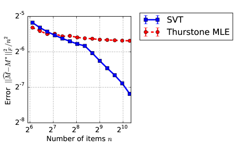
(a)		(b)

Figure 1: (a) Construction of a “bad” matrix: for $n$ divisible by $4$, form the matrix $M^{*}\in\mathbb{R}^{n\times n}$ shown, where each block has dimensions $n/4\times n/4$. (b) Estimation for a class of SST matrices that are far from the parametric models. The parametric model (Thurstone MLE) yields a poor fit, whereas fitting using the singular value thresholding (SVT) estimator, which allows for estimates over the full SST class, leads to consistent estimation.

The lower bound on approximation quality guaranteed by Proposition 1 means that any parametric estimator of the matrix $M^{*}$ should perform poorly. This expectation is confirmed by the simulation results in panel (b) of Figure 1. After generating observations from a “bad matrix” over a range of $n$, we fit the data set using either the maximum likelihood estimate in the Thurstone model, or the singular value thresholding (SVT) estimator, to be discussed in Section 3.2. For each estimator $\widehat{M}$, we plot the rescaled Frobenius norm error $\frac{|\!|\!|\widehat{M}-M^{*}|\!|\!|_{{\mbox{\tiny{F}}}}^{2}}{n^{2}}$ versus the sample size. Consistent with the lower bound (6), the error in the Thurstone-based estimator stays bounded above a universal constant. In contrast, the SVT error goes to zero with $n$, and as our theory in the sequel shows, the rate at which the error decays is at least as fast as $1/\sqrt{n}$.

3 Main results

Thus far, we have introduced two classes of models for matrices of pairwise comparison probabilities. Our main results characterize the rates of estimation associated with different subsets of these classes, using either optimal estimators (that we suspect are not polynomial-time computable), or more computationally efficient estimators that can be computed in polynomial-time.

3.1 Characterization of the minimax risk

We begin by providing a result that characterizes the minimax risk in squared Frobenius norm over the class $\mathbb{C}_{\mbox{\scalebox{0.5}{{SST}}}}$ of SST matrices. The minimax risk is defined by taking an infimum over the set of all possible estimators, which are measurable functions $Y\mapsto\widetilde{M}\in[0,1]^{n\times n}$. Here the data matrix $Y\in\{0,1\}^{n\times n}$ is drawn from the observation model (1).

Theorem 1.

There are universal constants $0<c_{\ell}<c_{u}$ such that

$$\frac{c_{\ell}}{n}\;\leq\;\inf_{\widetilde{M}}\sup_{M^{*}\in\mathbb{C}_{\mbox{\scalebox{0.5}{{SST}}}}}\frac{1}{n^{2}}\mathbb{E}[|\!|\!|\widetilde{M}-M^{*}|\!|\!|_{{\mbox{\tiny{F}}}}^{2}]\;\leq\;c_{u}\frac{\log^{2}(n)}{n},$$ (7)

where the infimum ranges over all measurable functions $\widetilde{M}$ of the observed matrix $Y$.

We prove this theorem in Section 5.1. The proof of the lower bound is based on extracting a particular subset of the class $\mathbb{C}_{\mbox{\scalebox{0.5}{{SST}}}}$ such that any matrix in this subset has at least $n$ positions that are unconstrained, apart from having to belong to the interval $[{\frac{1}{2}},1]$. We can thus conclude that estimation of the full matrix is at least as hard as estimating $n$ Bernoulli parameters belonging to the interval $[{\frac{1}{2}},1]$ based on a single observation per number. This reduction leads to an $\Omega(n^{-1})$ lower bound, as stated.

Proving an upper bound requires substantially more effort. In particular, we establish it via careful analysis of the constrained least-squares estimator

$$\widehat{M}\in\operatornamewithlimits{arg~{}min}_{M\in\mathbb{C}_{\mbox{\scalebox{0.5}{{SST}}}}}|\!|\!|Y-M|\!|\!|_{{\mbox{\tiny{F}}}}^{2}.$$ (8a)

In particular, we prove that there are universal constants $$(c_{0},c_{1},c_{2}) M^{*}\in\mathbb{C}_{\mbox{\scalebox{0.5}{{SST}}}}$$ such that, for any matrix , this estimator satisfies the high probability bound

$$\mathbb{P}\Big{[}\frac{1}{n^{2}}|\!|\!|\widehat{M}-M^{*}|\!|\!|_{{\mbox{\tiny{F}}}}^{2}\geq c_{0}\frac{\log^{2}(n)}{n}\Big{]} \leq c_{1}e^{-c_{2}n}.$$ (8b)

Since the entries of $\widehat{M}$ and $M^{*}$ all lie in the interval $[0,1]$, integrating this tail bound leads to the stated upper bound (7) on the expected mean-squared error. Proving the high probability bound (8b) requires sharp control on a quantity known as the localized Gaussian complexity of the class $\mathbb{C}_{\mbox{\scalebox{0.5}{{SST}}}}$. We use Dudley’s entropy integral (e.g., [VDVW96, Corollary 2.2.8]) in order to derive an upper bound that is sharp up to a logarithmic factor; doing so in turn requires deriving upper bounds on the metric entropy of the class $\mathbb{C}_{\mbox{\scalebox{0.5}{{SST}}}}$ for which we leverage the prior work of Gao and Wellner [GW07].

We do not know whether the constrained least-squares estimator (8a) is computable in time polynomial in $n$, but we suspect not. This complexity is a consequence of the fact that the set $\mathbb{C}_{\mbox{\scalebox{0.5}{{SST}}}}$ is not convex, but is a union of $n!$ convex sets. Given this issue, it becomes interesting to consider the performance of alternative estimators that can be computed in polynomial-time.

3.2 Sharp analysis of singular value thresholding (SVT)

The first polynomial-time estimator that we consider is a simple estimator based on thresholding singular values of the observed matrix $Y$, and reconstructing its truncated singular value decomposition. For the full class $\mathbb{C}_{\mbox{\scalebox{0.5}{{SST}}}}$, Chatterjee [Cha14] analyzed the performance of such an estimator and proved that the squared Frobenius error decays as $\mathcal{O}(n^{-\frac{1}{4}})$ uniformly over $\mathbb{C}_{\mbox{\scalebox{0.5}{{SST}}}}$. In this section, we prove that its error decays as $\mathcal{O}(n^{-{\frac{1}{2}}})$, again uniformly over $\mathbb{C}_{\mbox{\scalebox{0.5}{{SST}}}}$, and moreover, that this upper bound is unimprovable.

Let us begin by describing the estimator. Given the observation matrix $Y\in\mathbb{R}^{n\times n}$, we can write its singular value decomposition as $Y=UDV^{T}$, where the $(n\times n)$ matrix $D$ is diagonal, whereas the $(n\times n)$ matrices $U$ and $V$ are orthonormal. Given a threshold level $\lambda_{n}>0$, the soft-thresholded version of a diagonal matrix $D$ is the diagonal matrix $T_{\lambda_{n}}(D)$ with values

$$[T_{\lambda_{n}}(D)]_{jj} =\max\{0,D_{jj}-\lambda_{n}\}\quad\mbox{for every integer $j\in[1,n]$}.$$ (9)

With this notation, the soft singular-value-thresholded (soft-SVT) version of $Y$ is given by $T_{\lambda_{n}}(Y)=UT_{\lambda_{n}}(D)V^{T}$. The following theorem provides a bound on its squared Frobenius error:

Theorem 2.

There are universal positive constants $(c_{u},c_{0},c_{1})$ such that the soft-SVT estimator ${\widehat{M}}_{\lambda_{n}}=T_{\lambda_{n}}(Y)$ with $\lambda_{n}=2.1\sqrt{n}$ satisfies the bound

$$\mathbb{P}\Big{[}\frac{1}{n^{2}}|\!|\!|{\widehat{M}}_{\lambda_{n}}-M^{*}|\!|\!|_{{\mbox{\tiny{F}}}}^{2}\geq\frac{c_{u}}{\sqrt{n}}\Big{]} \leq c_{0}e^{-c_{1}n}$$ (10a)

for any $$M^{*}\in\mathbb{C}_{\mbox{\scalebox{0.5}{{SST}}}} c_{\ell}>0 \lambda_{n}$$. Moreover, there is a universal constant such that for any choice of , we have

$$\sup_{M^{*}\in\mathbb{C}_{\mbox{\scalebox{0.5}{{SST}}}}}\frac{1}{n^{2}}|\!|\!|{\widehat{M}}_{\lambda_{n}}-M^{*}|\!|\!|_{{\mbox{\tiny{F}}}}^{2}\geq\frac{c_{\ell}}{\sqrt{n}}.$$ (10b)

A few comments on this result are in order. Since the matrices ${\widehat{M}}_{\lambda_{n}}$ and $M^{*}$ have entries in the unit interval $[0,1]$, the normalized squared error $\frac{1}{n^{2}}|\!|\!|{\widehat{M}}_{\lambda_{n}}-M^{*}|\!|\!|_{{\mbox{\tiny{F}}}}^{2}$ is at most $1$. Consequently, by integrating the the tail bound (10a), we find that

$$\sup_{M^{*}\in\mathbb{C}_{\mbox{\scalebox{0.5}{{SST}}}}}\mathbb{E}[\frac{1}{n^{2}}|\!|\!|{\widehat{M}}_{\lambda_{n}}-M^{*}|\!|\!|_{{\mbox{\tiny{F}}}}^{2}] \leq\frac{c_{u}}{\sqrt{n}}+c_{0}e^{-c_{1}n}\;\leq\frac{c_{u}^{\prime}}{\sqrt{n}}.$$

On the other hand, the matching lower bound (10b) holds with probability one, meaning that the soft-SVT estimator has squared error of the order $1/\sqrt{n}$, irrespective of the realization of the noise.

To be clear, Chatterjee [Cha14] actually analyzed the hard-SVT estimator, which is based on the hard-thresholding operator

$$[H_{\lambda_{n}}(D)]_{jj} =D_{jj}\;\mathbf{1}\{D_{jj}\geq\lambda_{n}\}.$$

Here $\mathbf{1}\{\cdot\}$ denotes the 0-1-valued indicator function. In this setting, the hard-SVT estimator is simply, $H_{\lambda_{n}}(Y)=UH_{\lambda_{n}}(D)V^{T}$. With essentially the same choice of $\lambda_{n}$ as above, Chatterjee showed that the estimate $H_{\lambda_{n}}(Y)$ has a mean-squared error of $\mathcal{O}(n^{-1/4})$. One can verify that the proof of Theorem 2 in our paper goes through for the hard-SVT estimator as well. Consequently the performance of the hard-SVT estimator is of the order $\Theta(n^{-1/2})$, and is identical to that of the soft-thresholded version up to universal constants.

Note that the hard and soft-SVT estimators return matrices that may not lie in the SST class $\mathbb{C}_{\mbox{\scalebox{0.5}{{SST}}}}$. In a companion paper [SBW16], we provide an alternative computationally-efficient estimator with similar statistical guarantees that is guaranteed to return a matrix in the SST class.

Together the upper and lower bounds of Theorem 2 provide a sharp characterization of the behavior of the soft/hard SVT estimators. On the positive side, these are easily implementable estimators that achieve a mean-squared error bounded by $\mathcal{O}(1/\sqrt{n})$ uniformly over the entire class $\mathbb{C}_{\mbox{\scalebox{0.5}{{SST}}}}$. On the negative side, this rate is slower than the $\mathcal{O}(\log^{2}n/n)$ rate achieved by the least-squares estimator, as in Theorem 1.

In conjunction, Theorems 1 and 2 raise a natural open question: is there a polynomial-time estimator that achieves the minimax rate uniformly over the family $\mathbb{C}_{\mbox{\scalebox{0.5}{{SST}}}}$? We do not know the answer to this question, but the following subsections provide some partial answers by analyzing some polynomial-time estimators that (up to logarithmic factors) achieve the optimal $\tilde{\mathcal{O}}(1/n)$-rate over some interesting sub-classes of $\mathbb{C}_{\mbox{\scalebox{0.5}{{SST}}}}$. In the next two sections, we turn to results of this type.

3.3 Optimal rates for high SNR subclass

In this section, we describe a multi-step polynomial-time estimator that (up to logarithmic factors) can achieve the optimal $\tilde{\mathcal{O}}(1/n)$ rate over an interesting subclass of $\mathbb{C}_{\mbox{\scalebox{0.5}{{SST}}}}$. This subset corresponds to matrices $M$ that have a relatively high signal-to-noise ratio (SNR), meaning that no entries of $M$ fall within a certain window of $1/2$. More formally, for some $\gamma\in(0,{\frac{1}{2}})$, we define the class

$$\mathbb{C}_{\mbox{\scalebox{0.5}{{HIGH}}}}(\gamma)=\big{\{}M\in\mathbb{C}_{\mbox{\scalebox{0.5}{{SST}}}}\,\mid\,\max(M_{ij},M_{ji})\geq 1/2+\gamma~{}~{}\forall~{}~{}i\neq j\big{\}}.$$ (11)

By construction, for any matrix $\mathbb{C}_{\mbox{\scalebox{0.5}{{HIGH}}}}(\gamma)$, the amount of information contained in each observation is bounded away from zero uniformly in $n$, as opposed to matrices in which some large subset of entries have values equal (or arbitrarily close) to ${\frac{1}{2}}$. In terms of estimation difficulty, this SNR restriction does not make the problem substantially easier: as the following theorem shows, the minimax mean-squared error remains lower bounded by a constant multiple of $1/n$. Moreover, we can demonstrate a polynomial-time algorithm that achieves this optimal mean squared error up to logarithmic factors.

The following theorem applies to any fixed $\gamma\in(0,{\frac{1}{2}}]$ independent of $n$, and involves constants $(c_{\ell},c_{u},c)$ that may depend on $\gamma$ but are independent of $n$.

Theorem 3.

There is a constant $c_{\ell}>0$ such that

$$\inf_{\widetilde{M}}\sup_{M^{*}\in\mathbb{C}_{\mbox{\scalebox{0.5}{{HIGH}}}}(\gamma)}\frac{1}{n^{2}}\mathbb{E}\big{[}|\!|\!|\widetilde{M}-M^{*}|\!|\!|_{{\mbox{\tiny{F}}}}^{2}] \geq\frac{c_{\ell}}{n},$$ (12a)

where the infimum ranges over all estimators. Moreover, there is a two-stage estimator $$\widehat{M}$$, computable in polynomial-time, for which

$$\mathbb{P}\Big{[}\frac{1}{n^{2}}|\!|\!|\widehat{M}-M^{*}|\!|\!|_{{\mbox{\tiny{F}}}}^{2}\geq\frac{c_{u}\log^{2}(n)}{n}\Big{]} \leq\frac{c}{n^{2}},$$ (12b)

valid for any $$M^{*}\in\mathbb{C}_{\mbox{\scalebox{0.5}{{HIGH}}}}(\gamma)$$.

As before, since the ratio $\frac{1}{n^{2}}|\!|\!|\widehat{M}-M^{*}|\!|\!|_{{\mbox{\tiny{F}}}}^{2}$ is at most $1$, so the tail bound (12b) implies that

$$\sup_{M^{*}\in\mathbb{C}_{\mbox{\scalebox{0.5}{{HIGH}}}}(\gamma)}\frac{1}{n^{2}}\mathbb{E}[|\!|\!|\widehat{M}-M^{*}|\!|\!|_{{\mbox{\tiny{F}}}}^{2}] \leq\frac{c_{u}\log^{2}(n)}{n}+\frac{c}{n^{2}}\;\leq\;\frac{c_{u}^{\prime}\log^{2}(n)}{n}.$$ (13)

We provide the proof of this theorem in Section 5.3. As with our proof of the lower bound in Theorem 1, we prove the lower bound by considering the sub-class of matrices that are free only on the two diagonals just above and below the main diagonal. We now provide a brief sketch for the proof of the upper bound (12b). It is based on analyzing the following two-step procedure:

1. In the first step of algorithm, we find a permutation $\widehat{\pi}_{\mbox{\tiny{FAS}}}$ of the $n$ items that minimizes the total number of disagreements with the observations. (For a given ordering, we say that any pair of items $(i,j)$ are in disagreement with the observation if either $i$ is rated higher than $j$ in the ordering and $Y_{ij}=0$, or if $i$ is rated lower than $j$ in the ordering and $Y_{ij}=1$.) The problem of finding such a disagreement-minimizing permutation $\widehat{\pi}_{\mbox{\tiny{FAS}}}$ is commonly known as the minimum feedback arc set (FAS) problem. It is known to be NP-hard in the worst-case [ACN08, Alo06], but our set-up has additional probabilistic structure that allows for polynomial-time solutions with high probability. In particular, we call upon a polynomial-time algorithm due to Braverman and Mossel [BM08] that, under the model (11), is guaranteed to find the exact solution to the FAS problem with high probability. Viewing the FAS permutation $\widehat{\pi}_{\mbox{\tiny{FAS}}}$ as an approximation to the true permutation $\pi^{*}$, the novel technical work in this first step is show that $\widehat{\pi}_{\mbox{\tiny{FAS}}}$ is “good enough” for Frobenius norm estimation, in the sense that for any matrix $M^{*}\in\mathbb{C}_{\mbox{\scalebox{0.5}{{HIGH}}}}(\gamma)$, it satisfies the bound

   $$\frac{1}{n^{2}}|\!|\!|\pi^{*}(M^{*})-\widehat{\pi}_{\mbox{\tiny{FAS}}}(M^{*})|\!|\!|_{{\mbox{\tiny{F}}}}^{2} \leq\frac{c\log n}{n}$$ (14a)

   with high probability. In this statement, for any given permutation $$\pi \pi(M^{*}) M^{*} \pi \frac{1}{n^{2}}|\!|\!|\pi^{*}(M^{*})-\widehat{\pi}_{\mbox{\tiny{FAS}}}(M^{*})|\!|\!|_{{\mbox{\tiny{F}}}}^{2} \widehat{\pi}_{\mbox{\tiny{FAS}}} \pi^{*}$$, we have used to denote the matrix obtained by permuting the rows and columns of by . The term can be viewed in some sense as the bias in estimation incurred from using in place of .

2. Next we define $\mathbb{C}_{\mbox{\scalebox{0.5}{{BISO}}}}$ as the class of “bivariate isotonic” matrices, that is, matrices $M\in[0,1]^{n\times n}$ that satisfy the linear constraints $M_{ij}=1-M_{ji}$ for all $(i,j)\in[n]^{2}$, and $M_{k\ell}\geq M_{ij}$ whenever $k\leq i$ and $\ell\geq j$. This class corresponds to the subset of matrices $\mathbb{C}_{\mbox{\scalebox{0.5}{{SST}}}}$ that are faithful with respect to the identity permutation. Letting $\widehat{\pi}_{\mbox{\tiny{FAS}}}(\mathbb{C}_{\mbox{\scalebox{0.5}{{BISO}}}})=\{\widehat{\pi}_{\mbox{\tiny{FAS}}}(M),\,M\in\mathbb{C}_{\mbox{\scalebox{0.5}{{BISO}}}}\}$ denote the image of this set under $\widehat{\pi}_{\mbox{\tiny{FAS}}}$, the second step involves computing the constrained least-squares estimate

   $$\widehat{M}\in\operatornamewithlimits{arg~{}min}_{M\in\widehat{\pi}_{\mbox{\tiny{FAS}}}(\mathbb{C}_{\mbox{\scalebox{0.5}{{BISO}}}})}|\!|\!|Y-M|\!|\!|_{{\mbox{\tiny{F}}}}^{2}.$$ (14b)

   Since the set $\widehat{\pi}_{\mbox{\tiny{FAS}}}(\mathbb{C}_{\mbox{\scalebox{0.5}{{BISO}}}})$ is a convex polytope, with a number of facets that grows polynomially in $n$, the constrained quadratic program (14b) can be solved in polynomial-time. The final step in the proof of Theorem 3 is to show that the estimator $\widehat{M}$ also has mean-squared error that is upper bounded by a constant multiple of $\frac{\log^{2}(n)}{n}$.

Our analysis shows that for any fixed $\gamma\in(0,\frac{1}{2}]$, the proposed two-step estimator works well for any matrix $M^{*}\in\mathbb{C}_{\mbox{\scalebox{0.5}{{HIGH}}}}(\gamma)$. Since this two-step estimator is based on finding a minimum feedback arc set (FAS) in the first step, it is natural to wonder whether an FAS-based estimator works well over the full class $\mathbb{C}_{\mbox{\scalebox{0.5}{{SST}}}}$. Somewhat surprisingly the answer to this question turns out to be negative: we refer the reader to Appendix C for more intuition and details on why the minimal FAS estimator does not perform well over the full class.

3.4 Optimal rates for parametric subclasses

Let us now return to the class of parametric models $\mathbb{C}_{\mbox{\scalebox{0.5}{{PAR}}}}(F)$ introduced earlier in Section 2.3. As shown previously in Proposition 1, this class is much smaller than the class $\mathbb{C}_{\mbox{\scalebox{0.5}{{SST}}}}$, in the sense that there are models in $\mathbb{C}_{\mbox{\scalebox{0.5}{{SST}}}}$ that cannot be well-approximated by any parametric model. Nonetheless, in terms of minimax rates of estimation, these classes differ only by logarithmic factors. An advantage of the parametric class is that it is possible to achieve the $1/n$ minimax rate by using a simple, polynomial-time estimator. In particular, for any log concave function $F$, the maximum likelihood estimate $\widehat{w}_{\mbox{\tiny{ML}}}$ can be obtained by solving a convex program. This MLE induces a matrix estimate $M(\widehat{w}_{\mbox{\tiny{ML}}})$ via Equation (4), and the following result shows that this estimator is minimax-optimal up to constant factors.

Theorem 4.

Suppose that $F$ is strictly increasing, strongly log-concave and twice differentiable. Then there is a constant $c_{\ell}>0$, depending only on $F$, such that the minimax risk over $\mathbb{C}_{\mbox{\scalebox{0.5}{{PAR}}}}(F)$ is lower bounded as

$$\inf_{\widetilde{M}}\sup_{M^{*}\in\mathbb{C}_{\mbox{\scalebox{0.5}{{PAR}}}}(F)}\frac{1}{n^{2}}\mathbb{E}[|\!|\!|\widetilde{M}-M^{*}|\!|\!|_{{\mbox{\tiny{F}}}}^{2}]\geq\frac{c_{\ell}}{n},$$ (15a)

Conversely, there is a constant $$c_{u}\geq c_{\ell} F M(\widehat{w}_{\mbox{\tiny{ML}}})$$, depending only on , such that the matrix estimate induced by the MLE satisfies the bound

$$\sup_{M^{*}\in\mathbb{C}_{\mbox{\scalebox{0.5}{{PAR}}}}(F)}\frac{1}{n^{2}}\mathbb{E}[|\!|\!|M(\widehat{w}_{\mbox{\tiny{ML}}})-M^{*}|\!|\!|_{{\mbox{\tiny{F}}}}^{2}]\leq\frac{c_{u}}{n}.$$ (15b)

To be clear, the constants $(c_{\ell},c_{u})$ in this theorem are independent of $n$, but they do depend on the specific properties of the given function $F$. We note that the stated conditions on $F$ are true for many popular parametric models, including (for instance) the Thurstone and BTL models.

We provide the proof of Theorem 4 in Section 5.4. The lower bound (15a) is, in fact, stronger than the the lower bound in Theorem 1, since the supremum is taken over a smaller class. The proof of the lower bound in Theorem 1 relies on matrices that cannot be realized by any parametric model, so that we pursue a different route to establish the bound (15a). On the other hand, in order to prove the upper bound (15b), we make use of bounds on the accuracy of the MLE $\widehat{w}_{\mbox{\tiny{ML}}}$ from our own past work (see the paper [SBB⁺16]).

3.5 Extension to partial observations

We now consider the extension of our results to the setting in which not all entries of $Y$ are observed. Suppose instead that every entry of $Y$ is observed independently with probability $p_{\mathrm{obs}}$. In other words, the set of pairs compared is the set of edges of an Erdős-Rényi graph $\mathcal{G}(n,p_{\mathrm{obs}})$ that has the $n$ items as its vertices.

In this setting, we obtain an upper bound on the minimax risk of estimation by first setting $Y_{ij}={\frac{1}{2}}$ whenever the pair $(i,j)$ is not compared, then forming a new $(n\times n)$ matrix $Y^{\prime}$ as

$$Y^{\prime}:\,=\frac{1}{p_{\mathrm{obs}}}Y-\frac{1-p_{\mathrm{obs}}}{2p_{\mathrm{obs}}}11^{T},$$ (16a)

and finally computing the least squares solution

$$\widehat{M}\in\operatornamewithlimits{arg~{}min}\limits_{M\in\mathbb{C}_{\mbox{\scalebox{0.5}{{SST}}}}}|\!|\!|Y^{\prime}-M|\!|\!|_{{\mbox{\tiny{F}}}}^{2}.$$ (16b)

Likewise, the computationally-efficient singular value thresholding estimator is also obtained by thresholding the singular values of $Y^{\prime}$ with a threshold $\lambda_{n}=3\sqrt{\frac{n}{p_{\mathrm{obs}}}}$. See our discussion following Theorem 5 for the motivation underlying the transformed matrix $Y^{\prime}$.

The parametric estimators continue to operate on the original (partial) observations, first computing a maximum likelihood estimate $\widehat{w}_{\mbox{\tiny{ML}}}$ of $M^{*}$ using the observed data, and then computing the associated pairwise-comparison-probability matrix $M(\widehat{w}_{\mbox{\tiny{ML}}})$ via (4).

Theorem 5.

In the setting where each pair is observed with a probability $p_{\mathrm{obs}}$, there are positive universal constants $c_{\ell}$, $c_{u}$ and $c_{0}$ such that:

1. The minimax risk is sandwiched as

   $$\frac{c_{\ell}}{p_{\mathrm{obs}}n}\leq\inf_{\widetilde{M}}\sup_{M^{*}\in\mathbb{C}_{\mbox{\scalebox{0.5}{{SST}}}}}\frac{1}{n^{2}}\mathbb{E}[|\!|\!|\widetilde{M}-M^{*}|\!|\!|_{{\mbox{\tiny{F}}}}^{2}]\leq\frac{c_{u}(\log n)^{2}}{p_{\mathrm{obs}}n},$$ (17a)

   when $$p_{\mathrm{obs}}\geq\frac{c_{0}}{n}$$.

2. The soft-SVT estimator, ${\widehat{M}}_{\lambda_{n}}$ with $\lambda_{n}=3\sqrt{\frac{n}{p_{\mathrm{obs}}}}$, satisfies the bound

   $$\sup_{M^{*}\in\mathbb{C}_{\mbox{\scalebox{0.5}{{SST}}}}}\frac{1}{n^{2}}\mathbb{E}[|\!|\!|{\widehat{M}}_{\lambda_{n}}-M^{*}|\!|\!|_{{\mbox{\tiny{F}}}}^{2}] \leq\frac{c_{u}}{\sqrt{np_{\mathrm{obs}}}}.$$ (17b)

3. For a parametric sub-class based on a strongly log-concave and smooth $F$, the estimator $M(\widehat{w}_{\mbox{\tiny{ML}}})$ induced by the maximum likelihood estimate $\widehat{w}_{\mbox{\tiny{ML}}}$ of the parameter vector $w^{*}$ has mean-squared error upper bounded as

   $$\sup_{M^{*}\in\mathbb{C}_{\mbox{\scalebox{0.5}{{PAR}}}}(F)}\frac{1}{n^{2}}\mathbb{E}[|\!|\!|M(\widehat{w}_{\mbox{\tiny{ML}}})-M^{*}|\!|\!|_{{\mbox{\tiny{F}}}}^{2}]\leq\frac{c_{u}}{p_{\mathrm{obs}}n},$$ (17c)

   when $p_{\mathrm{obs}}\geq\frac{c_{0}(\log n)^{2}}{n}$.

The intuition behind the transformation (16a) is that the matrix $Y^{\prime}$ can equivalently be written in a linearized form as

$$Y^{\prime}=M^{*}+\frac{1}{p_{\mathrm{obs}}}W^{\prime},$$ (18a)

where $$W^{\prime}$$ has entries that are independent on and above the diagonal, satisfy skew-symmetry, and are distributed as

$$[W^{\prime}]_{ij}=\begin{cases}p_{\mathrm{obs}}({\frac{1}{2}}-[M^{*}]_{ij})+\frac{1}{2}&\qquad\mbox{with probability }p_{\mathrm{obs}}[M^{*}]_{ij}\\ p_{\mathrm{obs}}({\frac{1}{2}}-[M^{*}]_{ij})-\frac{1}{2}&\qquad\mbox{with probability }p_{\mathrm{obs}}(1-[M^{*}]_{ij})\\ p_{\mathrm{obs}}({\frac{1}{2}}-[M^{*}]_{ij})&\qquad\mbox{with probability }1-p_{\mathrm{obs}}.\end{cases}$$ (18b)

The proofs of the upper bounds exploit the specific relation (18a) between the observations $Y^{\prime}$ and the true matrix $M^{*}$, and the specific form of the additive noise (18b).

The result of Theorem 5(b) yields an affirmative answer to the question, originally posed by Chatterjee [Cha14], of whether or not the singular value thresholding estimator can yield a vanishing error when $p_{\mathrm{obs}}\leq\frac{1}{\sqrt{n}}$.

We note that we do not have an analogue of the high-SNR result in the partial observations case since having partial observations reduces the SNR. In general, we are interested in scalings of $p_{\mathrm{obs}}$ which allow $p_{\mathrm{obs}}\rightarrow 0$ as $n\rightarrow\infty$. The noisy-sorting algorithm of Braverman and Mossel [BM08] for the high-SNR case has computational complexity scaling as $e^{\gamma^{-4}}$, and hence is not computable in time polynomial in $n$ when $\gamma<(\log n)^{-\frac{1}{4}}$. This restriction disallows most interesting scalings of $p_{\mathrm{obs}}$ with $n$.

4 Simulations

In this section, we present results from simulations to gain a further understanding of the problem at hand, in particular to understand the rates of estimation under specific generative models. We investigate the performance of the soft-SVT estimator (Section 3.2) and the maximum likelihood estimator under the Thurstone model (Section 2.3). The output of the SVT estimator need not lie in the set $[0,1]^{n\times n}$ of matrices; in our implementation, we take a projection of the output of the SVT estimator on this set, which gives a constant factor reduction in the error.

In our simulations, we generate the ground truth $M^{*}$ in the following five ways:

• Uniform: The matrix $M^{*}$ is generated by drawing ${n\choose 2}$ values independently and uniformly at random in $[{\frac{1}{2}},1]$ and sorting them in descending order. The values are then inserted above the diagonal of an $(n\times n)$ matrix such that the entries decrease down a column or left along a row. We then make the matrix skew-symmetric and permute the rows and columns.

• Thurstone: The matrix $M^{*}\in[-1,1]^{n}$ is generated by first choosing $w^{*}$ uniformly at random from the set satisfying $\langle w^{*},\,1\rangle=0$. The matrix $M^{*}$ is then generated from $w^{*}$ via Equation (4) with $F$ chosen as the CDF of the standard normal distribution.

• Bradley-Terry-Luce (BTL): Identical to the Thurstone case, except that $F$ is given by the sigmoid function.

• High SNR: A setting studied previously by Braverman and Mossel [BM08], in which the noise is independent of the items being compared. Some global order is fixed over the $n$ items, and the comparison matrix $M^{*}$ takes the values $M^{*}_{ij}=0.9=1-M^{*}_{ji}$ for every pair $(i,j)$ where $i$ is ranked above $j$ in the underlying ordering. The entries on the diagonal are $0.5$.

• Independent bands: The matrix $M^{*}$ is chosen with diagonal entries all equal to $\frac{1}{2}$. Entries on diagonal band immediately above the diagonal itself are chosen i.i.d. and uniformly at random from $[{\frac{1}{2}},1]$. The band above is then chosen uniformly at random from the allowable set, and so on. The choice of any entry in this process is only constrained to be upper bounded by $1$ and lower bounded by the entries to its left and below. The entries below the diagonal are chosen to make the matrix skew-symmetric.

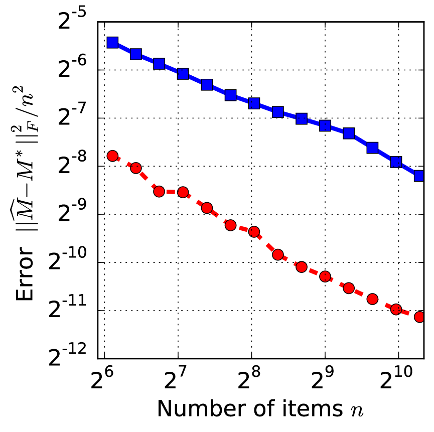
(a) Uniform

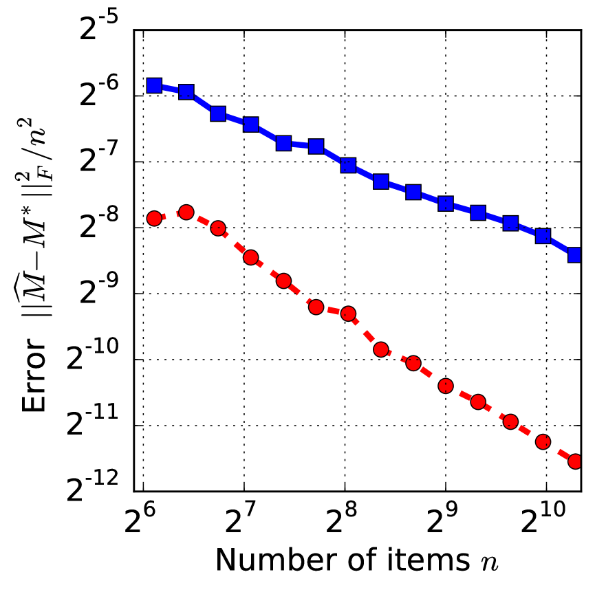
(b) Thurstone

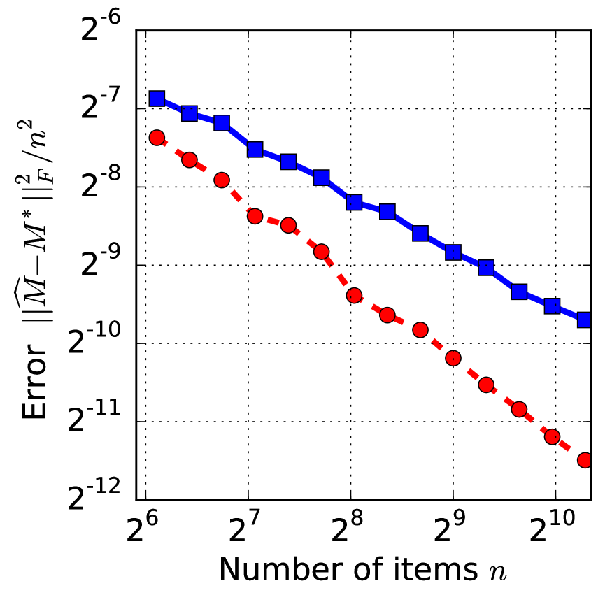
(c) BTL

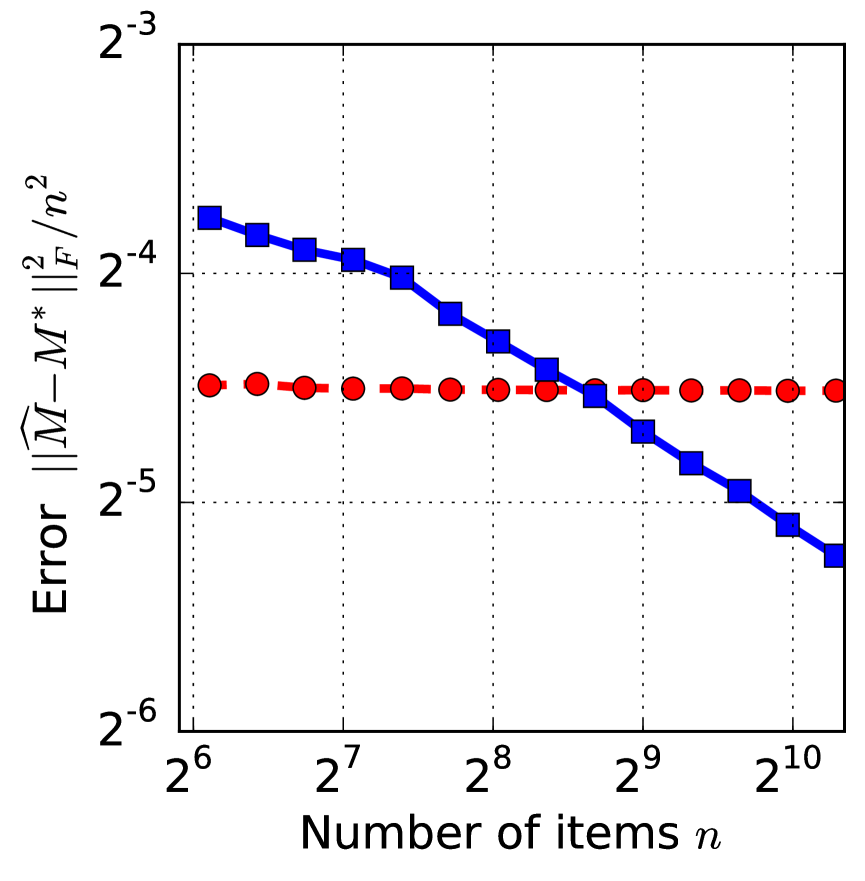
(d) High SNR

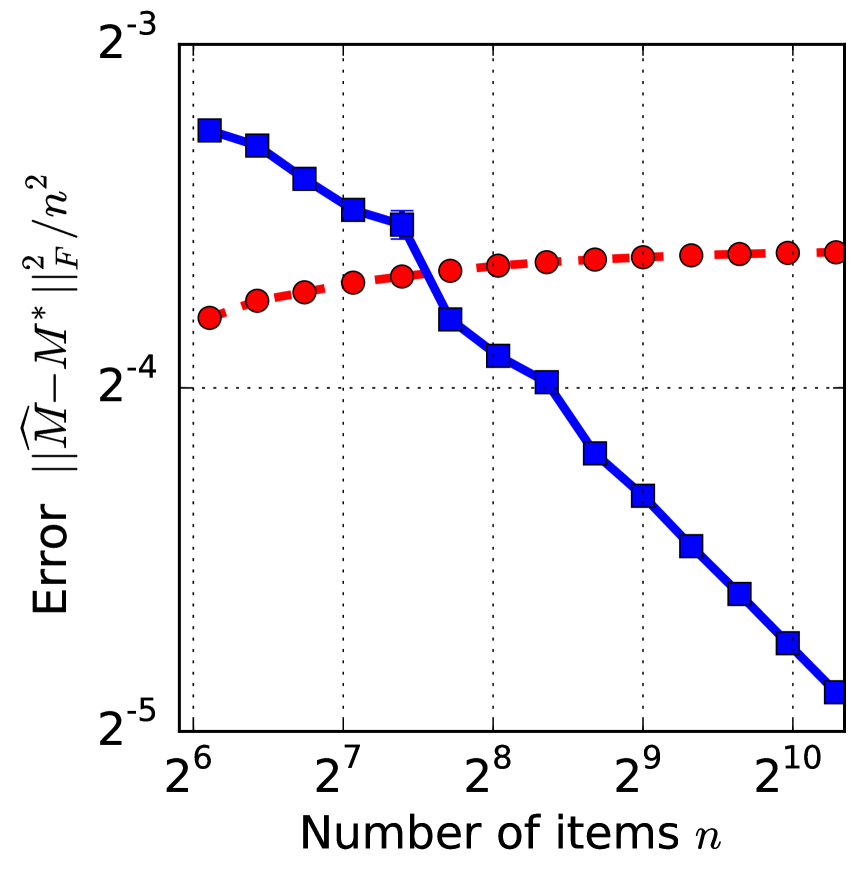
(e) Independent bands

Figure 2: Errors of singular value thresholding (SVT) estimator and the Thurstone MLE under different methods to generate $M^{*}$.

Figure 2 depicts the results of the simulations based on observations of the entire matrix $Y$. Each point is an average across $20$ trials. The error bars in most cases are too small and hence not visible. We see that the uniform case (Figure 2(a)) is favorable for both estimators, with the error scaling as $\mathcal{O}(\frac{1}{\sqrt{n}})$. With data generated from the Thurstone model, both estimators continue to perform well, and the Thurstone MLE yields an error of the order $\frac{1}{n}$ (Figure 2(b)). Interestingly, the Thurstone model also fits relatively well when data is generated via the BTL model (Figure 2(c)). This behavior is likely a result of operating in the near-linear regime of the logistic and the Gaussian CDF where the two curves are similar. In these two parametric settings, the SVT estimator has squared error strictly worse than order $\frac{1}{n}$ but better than $\frac{1}{\sqrt{n}}$. The Thurstone model, however, yields a poor fit for the model in the high-SNR (Figure 2(d)) and the independent bands (Figure 2(e)) cases, incurring a constant error as compared to an error scaling as $\mathcal{O}(\frac{1}{\sqrt{n}})$ for the SVT estimator. We recall that the poor performance of the Thurstone estimator was also described previously in Proposition 1 and Figure 1.

In summary, we see that while the Thurstone MLE estimator gives minimax optimal rates of estimation when the underlying model is parametric, it can be inconsistent when the parametric assumptions are violated. On the other hand, the SVT estimator is robust to violations of parametric assumptions, and while it does not necessarily give minimax-optimal rates, it remains consistent across the entire SST class. Finally, we remark that our theory predicts that the least squares estimator, if implementable, would outperform both these estimators in terms of statistical error.

5 Proofs of main results

This section is devoted to the proofs of our main results–namely, Theorems 1 through 5. Throughout these and other proofs, we use the notation $\{c,c^{\prime},c_{0},C,C^{\prime}\}$ and so on to denote positive constants whose values may change from line to line. In addition, we assume throughout that $n$ is lower bounded by a universal constant so as to avoid degeneracies. For any square matrix $A\in\mathbb{R}^{n\times n}$, we let $\{\sigma_{1}(A),\ldots,\sigma_{n}(A)\}$ denote its singular values (ordered from largest to smallest), and similarly, for any symmetric matrix $M\in\mathbb{R}^{n\times n}$, we let $\{\lambda_{1}(M),\ldots,\lambda_{n}(M)\}$ denote its ordered eigenvalues. The identity permutation is one where item $i$ is the $i^{th}$ most preferred item, for every $i\in[n]$.

5.1 Proof of Theorem 1

This section is devoted to the proof of Theorem 1, including both the upper and lower bounds on the minimax risk in squared Frobenius norm.

5.1.1 Proof of upper bound

Define the difference matrix $\widehat{\Delta}$$:\,=$$\widehat{M}$- $M^{*}$ between $M^{*}$ and the optimal solution $\widehat{M}$ to the constrained least-squares problem. Since $\widehat{M}$ is optimal and $M^{*}$ is feasible, we must have $|\!|\!|Y-\widehat{M}|\!|\!|_{{\mbox{\tiny{F}}}}^{2}\leq|\!|\!|Y-M^{*}|\!|\!|_{{\mbox{\tiny{F}}}}^{2}$, and hence following some algebra, we arrive at the basic inequality

$$\frac{1}{2}|\!|\!|\widehat{\Delta}|\!|\!|_{{\mbox{\tiny{F}}}}^{2}\leq\langle\!\langle{\widehat{\Delta}},\;{W}\rangle\!\rangle,$$ (19)

where $W\in\mathbb{R}^{n\times n}$ is the noise matrix in the observation model (1), and $\langle\!\langle{A},\;{B}\rangle\!\rangle:\,=\operatorname{trace}(A^{T}B)$ denotes the trace inner product.

We introduce some additional objects that are useful in our analysis. The class of bivariate isotonic matrices $\mathbb{C}_{\mbox{\scalebox{0.5}{{BISO}}}}$ is defined as

$$\mathbb{C}_{\mbox{\scalebox{0.5}{{BISO}}}}:\,=\big{\{}M\in[0,1]^{n\times n}\mid\mbox{$M_{k\ell}\geq M_{ij}$ whenever $k\leq i$ and $\ell\geq j$}\big{\}}.$$ (20)

For a given permutation $\pi$ and matrix $M$, we let $\pi(M)$ denote the matrix obtained by applying $\pi$ to its rows and columns. We then define the set

$$\mathbb{C}_{\mbox{\scalebox{0.5}{{DIFF}}}} :\,=\Big{\{}\pi_{1}(M_{1})-\pi_{2}(M_{2})\mid\mbox{for some }M_{1},\;M_{2}\in\mathbb{C}_{\mbox{\scalebox{0.5}{{BISO}}}},\mbox{ and perm. $\pi_{1}$ and $\pi_{2}$}\Big{\}}.$$ (21)

corresponding to the set of difference matrices. Note that $\mathbb{C}_{\mbox{\scalebox{0.5}{{DIFF}}}}\subset[-1,1]^{n\times n}$ by construction. One can verify that for any $M^{*}\in\mathbb{C}_{\mbox{\scalebox{0.5}{{SST}}}}$, we are guaranteed the inclusion

$$\{M-M^{*}\mid M\in\mathbb{C}_{\mbox{\scalebox{0.5}{{SST}}}},~{}|\!|\!|M-M^{*}|\!|\!|_{{\mbox{\tiny{F}}}}\leq t\}\subset\mathbb{C}_{\mbox{\scalebox{0.5}{{DIFF}}}}\cap\{|\!|\!|D|\!|\!|_{{\mbox{\tiny{F}}}}\leq t\}.$$

Consequently, the error matrix $\widehat{\Delta}$ must belong to $\mathbb{C}_{\mbox{\scalebox{0.5}{{DIFF}}}}$, and so must satisfy the properties defining this set. Moreover, as we discuss below, the set $\mathbb{C}_{\mbox{\scalebox{0.5}{{DIFF}}}}$ is star-shaped, and this property plays an important role in our analysis.

For each choice of radius $t>0$, define the random variable

$$Z(t) :\,=\sup_{D\in\mathbb{C}_{\mbox{\scalebox{0.5}{{DIFF}}}},|\!|\!|D|\!|\!|_{{\mbox{\tiny{F}}}}\leq t}\langle\!\langle{D},\;{W}\rangle\!\rangle.$$ (22)

Using our earlier basic inequality (19), the Frobenius norm error $|\!|\!|\widehat{\Delta}|\!|\!|_{{\mbox{\tiny{F}}}}$ then satisfies the bound

$$\frac{1}{2}|\!|\!|\widehat{\Delta}|\!|\!|_{{\mbox{\tiny{F}}}}^{2} \leq\langle\!\langle{\widehat{\Delta}},\;{W}\rangle\!\rangle\;\leq\;Z\big{(}|\!|\!|\widehat{\Delta}|\!|\!|_{{\mbox{\tiny{F}}}}\big{)}.$$ (23)

Thus, in order to obtain a high probability bound, we need to understand the behavior of the random quantity $Z(\delta)$.

One can verify that the set $\mathbb{C}_{\mbox{\scalebox{0.5}{{DIFF}}}}$ is star-shaped, meaning that $\alpha D\in\mathbb{C}_{\mbox{\scalebox{0.5}{{DIFF}}}}$ for every $\alpha\in[0,1]$ and every $D\in\mathbb{C}_{\mbox{\scalebox{0.5}{{DIFF}}}}$. Using this star-shaped property, we are guaranteed that there is a non-empty set of scalars $\delta_{n}>0$ satisfying the critical inequality

$$\mathbb{E}[Z(\delta_{n})] \leq\frac{\delta_{n}^{2}}{2}.$$ (24)

Our interest is in the smallest (strictly) positive solution $\delta_{n}$ to the critical inequality (24), and moreover, our goal is to show that for every $t\geq\delta_{n}$, we have $|\!|\!|\widehat{\Delta}|\!|\!|_{{\mbox{\tiny{F}}}}\leq c\sqrt{t\delta_{n}}$ with probability at least $1-c_{1}e^{-c_{2}nt\delta_{n}}$.

For each $t>0$, define the “bad” event $\mathcal{A}_{t}$ as

$$\mathcal{A}_{t} =\big{\{}\exists\Delta\in\mathbb{C}_{\mbox{\scalebox{0.5}{{DIFF}}}}\mid|\!|\!|\Delta|\!|\!|_{{\mbox{\tiny{F}}}}\geq\sqrt{t\delta_{n}}\quad\mbox{and}\quad\langle\!\langle{\Delta},\;{W}\rangle\!\rangle\geq 2|\!|\!|\Delta|\!|\!|_{{\mbox{\tiny{F}}}}\sqrt{t\delta_{n}}\big{\}}.$$ (25)

Using the star-shaped property of $\mathbb{C}_{\mbox{\scalebox{0.5}{{DIFF}}}}$, it follows by a rescaling argument that

$$\mathbb{P}[\mathcal{A}_{t}]\leq\mathbb{P}\big{[}Z(\delta_{n})\geq 2\delta_{n}\sqrt{t\delta_{n}}\big{]}\qquad\mbox{for all $t\geq\delta_{n}$.}$$

The entries of $W$ lie in $[-1,1]$, are i.i.d. on and above the diagonal, are zero-mean, and satisfy skew-symmetry. Moreover, the function $W\mapsto Z(t)$ is convex and Lipschitz with parameter $t$. Consequently, from known concentration bounds(e.g., [Led01, Theorem 5.9], [Sam00]) for convex Lipschitz functions, we have

$$\mathbb{P}\big{[}Z(\delta_{n})\geq\mathbb{E}[Z(\delta_{n})]+\sqrt{t\delta_{n}}\delta_{n}\big{]} \leq 2e^{-c_{1}t\delta_{n}}\qquad\mbox{for all $t\geq\delta_{n}$.}$$

By the definition of $\delta_{n}$, we have $\mathbb{E}[Z(\delta_{n})]\leq\delta_{n}^{2}\leq\delta_{n}\sqrt{t\delta_{n}}$ for any $t\geq\delta_{n}$, and consequently

$$\mathbb{P}[\mathcal{A}_{t}] \leq\mathbb{P}[Z(\delta_{n})\geq 2\delta_{n}\sqrt{t\delta_{n}}\big{]}\;\leq\;2e^{-c_{1}t\delta_{n}}\quad\mbox{for all $t\geq\delta_{n}$.}$$

Consequently, either $|\!|\!|\widehat{\Delta}|\!|\!|_{{\mbox{\tiny{F}}}}\leq\sqrt{t\delta_{n}}$, or we have $|\!|\!|\widehat{\Delta}|\!|\!|_{{\mbox{\tiny{F}}}}>\sqrt{t\delta_{n}}$. In the latter case, conditioning on the complement $\mathcal{A}_{t}^{c}$, our basic inequality implies that $\frac{1}{2}|\!|\!|\widehat{\Delta}|\!|\!|_{{\mbox{\tiny{F}}}}^{2}\leq 2|\!|\!|\widehat{\Delta}|\!|\!|_{{\mbox{\tiny{F}}}}\sqrt{t\delta_{n}}$, and hence $|\!|\!|\widehat{\Delta}|\!|\!|_{{\mbox{\tiny{F}}}}\leq 4\sqrt{t\delta_{n}}$ with probability at least $1-2e^{-c_{1}t\delta_{n}}$. Putting together the pieces yields that

$$|\!|\!|\widehat{\Delta}|\!|\!|_{{\mbox{\tiny{F}}}}\leq c_{0}\sqrt{t\delta_{n}}$$ (26)

with probability at least $1-2e^{-c_{1}t\delta_{n}}$ for every $t\geq\delta_{n}$.

In order to determine a feasible $\delta_{n}$ satisfying the critical inequality (24), we need to bound the expectation $\mathbb{E}[Z(\delta_{n})]$. We do using Dudley’s entropy integral and bounding the metric entropies of certain sub-classes of matrices. In particular, the remainder of this section is devoted to proving the following claim:

Lemma 1.

There is a universal constant $C$ such that

$$\mathbb{E}[Z(t)] \leq C\,\Big{\{}n\log^{2}(n)+t\,\sqrt{n\log n}\Big{\}},$$ (27)

for all $t\in[0,2n]$.

Given this lemma, we see that the critical inequality (24) is satisfied with $\delta_{n}=C^{\prime}\sqrt{n}\log n$. Consequently, from our bound (26), there are universal positive constants $C^{\prime\prime}$ and $c_{1}$ such that

$$\frac{|\!|\!|\widehat{\Delta}|\!|\!|_{{\mbox{\tiny{F}}}}^{2}}{n^{2}} \leq C^{\prime\prime}\frac{\log^{2}(n)}{n},$$

with probability at least $1-2e^{-c_{1}n(\log n)^{2}}$, which completes the proof.

Proof of Lemma 1: It remains to prove Lemma 1, and we do so by using Dudley’s entropy integral, as well as some auxiliary results on metric entropy. We use the notation $\log N(\epsilon,\mathbb{C},\rho)$ to denote the $\epsilon$ metric entropy of the class $\mathbb{C}$ in the metric $\rho$. Our proof requires the following auxiliary lemma:

Lemma 2.

For every $\epsilon>0$, we have the metric entropy bound

$$\log N(\epsilon,\mathbb{C}_{\mbox{\scalebox{0.5}{{DIFF}}}},|\!|\!|.|\!|\!|_{{\mbox{\tiny{F}}}}) \leq 9\frac{n^{2}}{\epsilon^{2}}\big{(}\log\frac{n}{\epsilon}\big{)}^{2}+9n\log n.$$

See the end of this section for the proof of this claim. Letting $\mathbb{B}_{F}(t)$ denote the Frobenius norm ball of radius $t$, the truncated form of Dudley’s entropy integral inequality (e.g., [VDVW96, Corollary 2.2.8]) yields that the mean $\mathbb{E}[Z(t)]$ is upper bounded as

$$\mathbb{E}[Z(t)]] \leq c\;\inf_{\delta\in[0,n]}\Big{\{}n\delta+\int_{\frac{\delta}{2}}^{t}\sqrt{\log N(\epsilon,\mathbb{C}_{\mbox{\scalebox{0.5}{{DIFF}}}}\cap\mathbb{B}_{F}(t),|\!|\!|.|\!|\!|_{{\mbox{\tiny{F}}}})}d\epsilon\Big{\}}$$

$$\leq c\;\Big{\{}n^{-8}+\int_{\frac{1}{2}n^{-9}}^{t}\sqrt{\log N(\epsilon,\mathbb{C}_{\mbox{\scalebox{0.5}{{DIFF}}}},|\!|\!|.|\!|\!|_{{\mbox{\tiny{F}}}})}d\epsilon\Big{\}},$$ (28)

where the second step follows by setting $\delta=n^{-9}$, and making use of the set inclusion $(\mathbb{C}_{\mbox{\scalebox{0.5}{{DIFF}}}}\cap\mathbb{B}_{F}(t))\subseteq\mathbb{C}_{\mbox{\scalebox{0.5}{{DIFF}}}}$. For any $\epsilon\geq\frac{1}{2}n^{-9}$, applying Lemma 2 yields the upper bound

$$\sqrt{\log N(\epsilon,\mathbb{C}_{\mbox{\scalebox{0.5}{{DIFF}}}},|\!|\!|.|\!|\!|_{{\mbox{\tiny{F}}}})}\leq c\Big{\{}\frac{n}{\epsilon}\log\frac{n}{\epsilon}+\sqrt{n\log n}\Big{\}}.$$

Over the range $\epsilon\geq n^{-9}/2$, we have $\log\frac{n}{\epsilon}\leq c\log n$, and hence

$$\sqrt{\log N(\epsilon,\mathbb{C}_{\mbox{\scalebox{0.5}{{DIFF}}}},|\!|\!|.|\!|\!|_{{\mbox{\tiny{F}}}})}\leq c\Big{\{}\frac{n}{\epsilon}\log n+\sqrt{n\log n}\Big{\}}.$$

Substituting this bound into our earlier inequality (28) yields

$$\mathbb{E}[Z(t)] \leq c\Big{\{}n^{-8}+\big{(}n\log n\big{)}\log(nt)+t\sqrt{n\log n}\Big{\}}$$

$$\stackrel{{\scriptstyle(i)}}{{\leq}}c\Big{\{}\big{(}n\log n\big{)}\log(n^{2})+t\sqrt{n\log n}\Big{\}}$$

$$\leq c\Big{\{}n\log^{2}(n)+t\sqrt{n\log n}\Big{\}},$$

where step (i) uses the upper bound $t\leq 2n$.

The only remaining detail is to prove Lemma 2.

Proof of Lemma 2:

We first derive an upper bound on the metric entropy of the class $\mathbb{C}_{\mbox{\scalebox{0.5}{{BISO}}}}$ defined previously in equation (20). In particular, we do so by relating it to the set of all bivariate monotonic functions on the square $[0,1]\times[0,1]$. Denoting this function class by ${\cal F}$, for any matrix $M\in\mathbb{C}_{\mbox{\scalebox{0.5}{{BISO}}}}$, we define a function $g_{M}\in{\cal F}$ via

$$g_{M}(x,y)=M_{\lceil n(1-x)\rceil,\lceil ny\rceil}.$$

In order to handle corner conditions, we set $M_{0,i}=M_{1,i}$ and $M_{i,0}=M_{i,1}$ for all $i$. With this definition, we have

$$\|g_{M}\|_{2}^{2}=\int_{x=0}^{1}\int_{y=0}^{1}(g_{M}(x,y))^{2}dxdy=\frac{1}{n^{2}}\sum_{i=1}^{n}\sum_{j=1}^{n}M_{i,j}^{2}=\frac{1}{n^{2}}|\!|\!|M|\!|\!|_{{\mbox{\tiny{F}}}}^{2}.$$

As a consequence, the metric entropy can be upper bounded as

$$\log N(\epsilon,\mathbb{C}_{\mbox{\scalebox{0.5}{{BISO}}}},|\!|\!|.|\!|\!|_{{\mbox{\tiny{F}}}}) \leq\;\log N\left(\frac{\epsilon}{n},{\cal F},\|.\|_{2}\right)$$

$$\stackrel{{\scriptstyle(i)}}{{\leq}}\;\frac{n^{2}}{\epsilon^{2}}\big{(}\log\frac{n}{\epsilon}\big{)}^{2},$$ (29)

where inequality (i) follows from Theorem 1.1 of Gao and Wellner [GW07].

We now bound the metric entropy of $\mathbb{C}_{\mbox{\scalebox{0.5}{{DIFF}}}}$ in terms of the metric entropy of $\mathbb{C}_{\mbox{\scalebox{0.5}{{BISO}}}}$. For any $\epsilon>0$, let $\mathbb{C}_{\mbox{\scalebox{0.5}{{BISO}}}}^{\epsilon}$ denote an $\epsilon$-covering set in $\mathbb{C}_{\mbox{\scalebox{0.5}{{BISO}}}}$ that satisfies the inequality (29). Consider the set

$$\mathbb{C}_{\mbox{\scalebox{0.5}{{DIFF}}}}^{\epsilon}:\,=\{\pi_{1}(M_{1})-\pi_{2}(M_{2})\mid\mbox{for some permutations $\pi_{1}$, $\pi_{2}$ and some $M_{1},M_{2}\in\mathbb{C}_{\mbox{\scalebox{0.5}{{BISO}}}}^{\epsilon/{2}}$}\}.$$

For any $D\in\mathbb{C}_{\mbox{\scalebox{0.5}{{DIFF}}}}$, we can write $D=\pi_{1}(M_{1}^{\prime})-\pi_{2}(M_{2}^{\prime})$ for some permutations $\pi_{1}$ and $\pi_{2}$ and some matrices $M_{1}^{\prime}$ and $M_{2}^{\prime}\in\mathbb{C}_{\mbox{\scalebox{0.5}{{BISO}}}}$. We know there exist matrices $M_{1},M_{2}\in\mathbb{C}_{\mbox{\scalebox{0.5}{{BISO}}}}^{\epsilon/{2}}$ such that $|\!|\!|M_{1}^{\prime}-M_{1}|\!|\!|_{{\mbox{\tiny{F}}}}\leq\epsilon/{2}$ and $|\!|\!|M_{2}^{\prime}-M_{2}|\!|\!|_{{\mbox{\tiny{F}}}}\leq\epsilon/{2}$. With these choices, we have $\pi_{1}(M_{1})-\pi_{2}(M_{2})\in\mathbb{C}_{\mbox{\scalebox{0.5}{{DIFF}}}}^{\epsilon}$, and moreover

$$|\!|\!|D-(\pi_{1}(M_{1})-\pi_{2}(M_{2}))|\!|\!|_{{\mbox{\tiny{F}}}}^{2} \leq 2|\!|\!|\pi_{1}(M_{1})-\pi_{1}(M_{1}^{\prime})|\!|\!|_{{\mbox{\tiny{F}}}}^{2}+2|\!|\!|\pi_{2}(M_{2})-\pi_{1}(M_{2}^{\prime})|\!|\!|_{{\mbox{\tiny{F}}}}^{2}$$

$$\leq\epsilon^{2}.$$

Thus the set $\mathbb{C}_{\mbox{\scalebox{0.5}{{DIFF}}}}^{\epsilon}$ forms an $\epsilon$-covering set for the class $\mathbb{C}_{\mbox{\scalebox{0.5}{{DIFF}}}}$. One can now count the number of elements in this set to find that

$$N(\epsilon,\mathbb{C}_{\mbox{\scalebox{0.5}{{DIFF}}}},|\!|\!|.|\!|\!|_{{\mbox{\tiny{F}}}})\leq\big{(}n!N(\epsilon/{2},\mathbb{C}_{\mbox{\scalebox{0.5}{{BISO}}}},|\!|\!|.|\!|\!|_{{\mbox{\tiny{F}}}})\big{)}^{2}.$$

Some straightforward algebraic manipulations yield the claimed result.

5.1.2 Proof of lower bound

We now turn to the proof of the lower bound in Theorem 1. We may assume that the correct row/column ordering is fixed and known to be the identity permutation. Here we are using the fact that revealing the knowledge of this ordering cannot make the estimation problem any harder. Recalling the definition (20) of the bivariate isotonic class $\mathbb{C}_{\mbox{\scalebox{0.5}{{BISO}}}}$, consider the subclass

$$\mathbb{C}_{\mbox{\scalebox{0.5}{{SST}}}}^{\prime}:\,=\{M\in\mathbb{C}_{\mbox{\scalebox{0.5}{{BISO}}}}\mid\mbox{$M_{i,j}=1$ when $j>i+1$ and $M_{i,j}=1-M_{j,i}$ when $j\leq i$}\}$$

Any matrix $M$ is this subclass can be identified with the vector $q=q(M)\in\mathbb{R}^{n-1}$ with elements $q_{i}:\,=M_{i,i+1}$. The only constraint imposed on $q(M)$ by the inclusion $M\in\mathbb{C}_{\mbox{\scalebox{0.5}{{SST}}}}$ is that $q_{i}\in[\frac{1}{2},1]$ for all $i=1,\ldots,n-1$.

In this way, we have shown that the difficulty of estimating $M^{*}\in\mathbb{C}_{\mbox{\scalebox{0.5}{{SST}}}}^{\prime}$ is at least as hard as that of estimating a vector $q\in[\frac{1}{2},1]^{n-1}$ based on observing the random vector $Y=\{Y_{1,2},\ldots,Y_{n-1,n}\}$ with independent coordinates, and such that each $Y_{i,i+1}\sim\operatorname{Ber}(q_{i})$. For this problem, it is easy to show that there is a universal constant $c_{\ell}>0$ such that

$$\inf_{\widehat{q}}\sup_{q\in[\frac{1}{2},1]^{n-1}}\mathbb{E}\Big{[}\|\widehat{q}-q\|_{2}^{2}\Big{]} \geq\frac{c_{\ell}}{2}n,$$

where the infimum is taken over all measurable functions $Y\mapsto\widehat{q}$. Putting together the pieces, we have shown that

$$\inf_{\widehat{M}}\sup_{M^{*}\in\mathbb{C}_{\mbox{\scalebox{0.5}{{SST}}}}}\frac{1}{n^{2}}\mathbb{E}[|\!|\!|\hat{M}-M^{*}|\!|\!|_{{\mbox{\tiny{F}}}}^{2}] \geq\frac{2}{n^{2}}\inf_{\widehat{q}}\sup_{q\in[0.5,1]^{n-1}}\mathbb{E}[\|\widehat{q}-q\|_{2}^{2}]\geq\frac{c_{\ell}}{n},$$

as claimed.

5.2 Proof of Theorem 2

Recall from equation (1) that we can write our observation model as $Y=M^{*}+W$, where $W\in\mathbb{R}^{n\times n}$ is a zero-mean matrix with entries that are drawn independently (except for the skew-symmetry condition) from the interval $[-1,1]$.

5.2.1 Proof of upper bound

Our proof of the upper bound hinges upon the following two lemmas.

Lemma 3.

If $\lambda_{n}\geq 1.01|\!|\!|W|\!|\!|_{{\mbox{\tiny{op}}}}$, then

$$|\!|\!|T_{\lambda_{n}}(Y)-M^{*}|\!|\!|_{{\mbox{\tiny{F}}}}^{2} \leq c\sum_{j=1}^{n}\min\big{\{}\lambda^{2}_{n},\sigma_{j}^{2}(M^{*})\big{\}},$$

where $c$ is a positive universal constant.

Our second lemma is an approximation-theoretic result:

Lemma 4.

For any matrix $M^{*}\in\mathbb{C}_{\mbox{\scalebox{0.5}{{SST}}}}$ and any $s\in\{1,2,\ldots,n-1\}$, we have

$$\frac{1}{n^{2}}\sum_{j=s+1}^{n}\sigma^{2}_{j}(M^{*}) \leq\frac{1}{s}.$$

See the end of this section for the proofs of these two auxiliary results.

Based on these two lemmas, it is easy to complete the proof of the theorem. The entries of $W$ are zero-mean with entries in the interval $[-1,1]$, are i.i.d. on and above the diagonal, and satisfy skew-symmetry. Consequently, we may apply Theorem 3.4 of Chatterjee [Cha14], which guarantees that

$$\mathbb{P}\Big{[}|\!|\!|W|\!|\!|_{{\mbox{\tiny{op}}}}>(2+t)\sqrt{n}\Big{]} \leq ce^{-f(t)n},$$

where $c$ is a universal constant, and the quantity $f(t)$ is strictly positive for each $t>0$. Thus, the choice $\lambda_{n}=2.1\sqrt{n}$ guarantees that $\lambda_{n}\geq 1.01|\!|\!|W|\!|\!|_{{\mbox{\tiny{op}}}}$ with probability at least $1-ce^{-cn}$, as is required for applying Lemma 3. Applying this lemma guarantees that the upper bound

$$|\!|\!|T_{\lambda_{n}}(Y)-M^{*}|\!|\!|_{{\mbox{\tiny{F}}}}^{2} \leq c\sum_{j=1}^{n}\min\big{\{}n,\sigma_{j}^{2}(M^{*})\big{\}}$$

hold with probability at least $1-c_{1}e^{-c_{2}n}$. From Lemma 4, with probability at least $1-c_{1}e^{-c_{2}n}$, we have

$$\frac{1}{n^{2}}|\!|\!|T_{\lambda_{n}}(Y)-M^{*}|\!|\!|_{{\mbox{\tiny{F}}}}^{2} \leq c\Big{\{}\frac{s}{n}+\frac{1}{s}\Big{\}}$$

for all $s\in\{1,\ldots,n\}$. Setting $s=\lceil\sqrt{n}\rceil$ and performing some algebra shows that

$$\mathbb{P}\Big{[}\frac{1}{n^{2}}|\!|\!|T_{\lambda_{n}}(Y)-M^{*}|\!|\!|_{{\mbox{\tiny{F}}}}^{2}>\frac{c_{u}}{\sqrt{n}}\Big{]} \leq c_{1}e^{-c_{2}n},$$

as claimed. Since $\frac{1}{n^{2}}|\!|\!|T_{\lambda_{n}}(Y)-M^{*}|\!|\!|_{{\mbox{\tiny{F}}}}^{2}\leq 1$, we are also guaranteed that

$$\frac{1}{n^{2}}\mathbb{E}[|\!|\!|T_{\lambda_{n}}(Y)-M^{*}|\!|\!|_{{\mbox{\tiny{F}}}}^{2}] \leq\frac{c_{u}}{\sqrt{n}}+c_{1}e^{-c_{2}n}\;\leq\frac{c_{u}^{\prime}}{\sqrt{n}}.$$

Proof of Lemma 3

Fix $\delta=0.01$. Let $b$ be the number of singular values of $M^{*}$ above $\frac{\delta}{1+\delta}\lambda_{n}$, and let $M^{*}_{b}$ be the version of $M^{*}$ truncated to its top $b$ singular values. We then have

$$|\!|\!|T_{\lambda_{n}}(Y)-M^{*}|\!|\!|_{{\mbox{\tiny{F}}}}^{2} \leq 2|\!|\!|T_{\lambda_{n}}(Y)-M^{*}_{b}|\!|\!|_{{\mbox{\tiny{F}}}}^{2}+2|\!|\!|M^{*}_{b}-M^{*}|\!|\!|_{{\mbox{\tiny{F}}}}^{2}$$

$$\leq 2\operatorname{rank}(T_{\lambda_{n}}(Y)-M^{*}_{b})|\!|\!|T_{\lambda_{n}}(Y)-M^{*}_{b}|\!|\!|_{{\mbox{\tiny{op}}}}^{2}+2\sum_{j=b+1}^{n}\sigma_{j}^{2}(M^{*}).$$

We claim that $T_{\lambda_{n}}(Y)$ has rank at most $b$. Indeed, for any $j\geq b+1$, we have

$$\sigma_{j}(Y) \leq\sigma_{j}(M^{*})+|\!|\!|W|\!|\!|_{{\mbox{\tiny{op}}}}\;\leq\;\lambda_{n},$$

where we have used the facts that $\sigma_{j}(M^{*})\leq\frac{\delta}{1+\delta}\lambda_{n}$ for every $j\geq b+1$ and $\lambda_{n}\geq(1+\delta)|\!|\!|W|\!|\!|_{{\mbox{\tiny{op}}}}$. As a consequence we have $\sigma_{j}(T_{\lambda_{n}}(Y))=0$, and hence $\operatorname{rank}(T_{\lambda_{n}}(Y)-M^{*}_{b})\leq 2b$. Moreover, we have

$$|\!|\!|T_{\lambda_{n}}(Y)-M^{*}_{b}|\!|\!|_{{\mbox{\tiny{op}}}} \leq|\!|\!|T_{\lambda_{n}}(Y)-Y|\!|\!|_{{\mbox{\tiny{op}}}}+|\!|\!|Y-M^{*}|\!|\!|_{{\mbox{\tiny{op}}}}+|\!|\!|M^{*}-M^{*}_{b}|\!|\!|_{{\mbox{\tiny{op}}}}$$

$$\leq\lambda_{n}+|\!|\!|W|\!|\!|_{{\mbox{\tiny{op}}}}+\frac{\delta}{1+\delta}\lambda_{n}$$

$$\leq 2\lambda_{n}.$$

Putting together the pieces, we conclude that

$$|\!|\!|T_{\lambda_{n}}(Y)-M^{*}|\!|\!|_{{\mbox{\tiny{F}}}}^{2} \leq 16b\lambda_{n}^{2}+2\sum_{j=b+1}^{n}\sigma_{j}^{2}(M^{*})\;\stackrel{{\scriptstyle(i)}}{{\leq}}\;C\sum_{j=1}^{n}\min\{\sigma_{j}^{2}(M^{*}),\lambda_{n}^{2}\},$$

for some constant $C$. Here inequality (i) follows since $\sigma_{j}(M^{*})\leq\frac{\delta}{1+\delta}\lambda_{n}$ whenever $j\geq b+1$ and $\sigma_{j}(M^{*})>\frac{\delta}{1+\delta}\lambda_{n}$ whenever $j\leq b$.

Proof of Lemma 4

In this proof, we make use of a construction due to Chatterjee [Cha14]. For a given matrix $M^{*}$, we can define the vector $t\in\mathbb{R}^{n}$ of row sums—namely, with entries $t_{i}=\sum_{j=1}^{n}M^{*}_{ij}$ for $i\in[n]$. Using this vector, we can define a rank $s$ approximation $M$ to the original matrix $M^{*}$ by grouping the rows according to the vector $t$ according to the following procedure:

• Observing that each $t_{i}\in[0,n]$, let us divide the full interval $[0,n]$ into $s$ groups—say of the form $[0,n/s),[n/s,2n/s),\ldots[(s-1)n/s,n]$. If $t_{i}$ falls into the interval $\alpha$ for some $\alpha\in[s]$, we then map row $i$ to the group $G_{\alpha}$ of indices.

• For each group $G_{\alpha}$, we choose a particular row index $k=k(\alpha)\in G_{\alpha}$ in an arbitrary fashion. For every other row index $i\in G_{\alpha}$, we set $M_{ij}=M_{kj}$ for all $j\in[n]$.

By construction, the matrix $M$ has at most $s$ distinct rows, and hence rank at most $s$. Let us now bound the Frobenius norm error in this rank $s$ approximation. Fixing an arbitrary group index $\alpha\in[s]$ and an arbitrary row in $i\in G_{\alpha}$, we then have

$$\sum_{j=1}^{n}(M^{*}_{ij}-M_{ij})^{2}\leq\sum_{j=1}^{n}|M^{*}_{ij}-M_{ij}|.$$

By construction, we either have $M^{*}_{ij}\geq M_{ij}$ for every $j\in[n]$, or $M^{*}_{ij}\leq M_{ij}$ for every $j\in[n]$. Thus, letting $k\in G_{\alpha}$ denote the chosen row, we are guaranteed that

$$\sum_{j=1}^{n}|M^{*}_{ij}-M_{ij}|\leq|t_{i}-t_{k}|\leq\frac{n}{s},$$

where we have used the fact the pair $(t_{i},t_{k})$ must lie in an interval of length at most $n/s$. Putting together the pieces yields the claim.

5.2.2 Proof of lower bound

We now turn to the proof of the lower bound in Theorem 2. We split our analysis into two cases, depending on the magnitude of $\lambda_{n}$.

Case 1:

First suppose that $\lambda_{n}\leq\frac{\sqrt{n}}{3}$. In this case, we consider the matrix $M^{*}:\,={\frac{1}{2}}11^{T}$ in which all items are equally good, so any comparison is simply a fair coin flip. Let the observation matrix $Y\in\{0,1\}^{n\times n}$ be arbitrary. By definition of the singular value thresholding operation, we have $|\!|\!|Y-T_{\lambda_{n}}(Y)|\!|\!|_{{\mbox{\tiny{op}}}}\leq\lambda_{n}$, and hence the SVT estimator ${\widehat{M}}_{\lambda_{n}}=T_{\lambda_{n}}(Y)$ has Frobenius norm at most

$$|\!|\!|Y-{\widehat{M}}_{\lambda_{n}}|\!|\!|_{{\mbox{\tiny{F}}}}^{2}\leq n\lambda_{n}^{2} \leq\frac{n^{2}}{9}.$$

Since $M^{*}\in\{{\frac{1}{2}}\}^{n\times n}$ and $Y\in\{0,1\}^{n\times n}$, we are guaranteed that $|\!|\!|M^{*}-Y|\!|\!|_{{\mbox{\tiny{F}}}}=\frac{n}{2}$. Applying the triangle inequality yields the lower bound

$$|\!|\!|{\widehat{M}}_{\lambda_{n}}-M^{*}|\!|\!|_{{\mbox{\tiny{F}}}}\;\geq\>|\!|\!|M^{*}-Y|\!|\!|_{{\mbox{\tiny{F}}}}-|\!|\!|{\widehat{M}}_{\lambda_{n}}-Y|\!|\!|_{{\mbox{\tiny{F}}}}\;\geq\frac{n}{2}-\frac{n}{3}\;=\;\frac{n}{6}.$$

Case 2:

Otherwise, we may assume that $\lambda_{n}>\frac{\sqrt{n}}{3}$. Consider the matrix $M^{*}\in\mathbb{R}^{n\times n}$ with entries

$$[M^{*}]_{ij}=\begin{cases}1&\mbox{if~{}}i>j\\ {\frac{1}{2}}&\mbox{if~{}}i=j\\ 0&\mbox{if~{}}i<j.\end{cases}$$ (30)

By construction, the matrix $M^{*}$ corresponds to the degenerate case of noiseless comparisons.

Consider the matrix $Y\in\mathbb{R}^{n\times n}$ generated according to the observation model (1). (To be clear, all of its off-diagonal entries are deterministic, whereas the diagonal is population with i.i.d. Bernoulli variates.) Our proof requires the following auxiliary result regarding the singular values of $Y$:

Lemma 5.

The singular values of the observation matrix $Y\in\mathbb{R}^{n\times n}$ generated by the noiseless comparison matrix $M^{*}$ satisfy the bounds

$$\frac{n}{4\pi(i+1)}-{\frac{1}{2}}\leq\sigma_{n-i-1}(Y)\leq\frac{n}{\pi(i-1)}+{\frac{1}{2}}\qquad\mbox{for all integers $i\in[1,\frac{n}{6}-1]$.}$$

We prove this lemma at the end of this section.

Taking it as given, we get that $\sigma_{n-i-1}(Y)\leq\frac{\sqrt{n}}{3}$ for every integer $i\geq 2\sqrt{n}$, and $\sigma_{n-i}(Y)\geq\frac{n}{50i}$ for every integer $i\in[1,\frac{n}{25}]$. It follows that

$$\sum_{i=1}^{n}(\sigma_{i}(Y))^{2}\mathbf{1}\{\sigma_{i}(Y)\leq\frac{\sqrt{n}}{3}\} \geq\frac{n^{2}}{2500}\sum_{i=2\sqrt{n}}^{\frac{n}{25}}\frac{1}{i^{2}}\;\geq\;cn^{\frac{3}{2}},$$

for some universal constant $c>0$. Recalling that $\lambda_{n}\geq\frac{\sqrt{n}}{3}$, we have the lower bound $|\!|\!|Y-{\widehat{M}}_{\lambda_{n}}|\!|\!|_{{\mbox{\tiny{F}}}}^{2}\geq cn^{\frac{3}{2}}$. Furthermore, since the observations (apart from the diagonal entries) are noiseless, we have $|\!|\!|Y-M^{*}|\!|\!|_{{\mbox{\tiny{F}}}}^{2}\leq\frac{n}{4}$. Putting the pieces together yields the lower bound

$$|\!|\!|{\widehat{M}}_{\lambda_{n}}-M^{*}|\!|\!|_{{\mbox{\tiny{F}}}}\;\geq|\!|\!|{\widehat{M}}_{\lambda_{n}}-Y|\!|\!|_{{\mbox{\tiny{F}}}}-|\!|\!|M^{*}-Y|\!|\!|_{{\mbox{\tiny{F}}}} \geq\;cn^{\frac{3}{4}}-\frac{\sqrt{n}}{2}\;\geq\;c^{\prime}n^{\frac{3}{4}},$$

where the final step holds when $n$ is large enough (i.e., larger than a universal constant).

Proof of Lemma 5:

Instead of working with the original observation matrix $Y$, it is convenient to work with a transformed version. Define the matrix $\bar{Y}:\,=Y-\mbox{diag}(Y)+I_{n}$, so that the matrix $\bar{Y}$ is identical to $Y$ except that all its diagonal entries are set to $1$. Using this intermediate object, define the $(n\times n)$ matrix

$$\widetilde{Y} :\,=(\bar{Y}(\bar{Y})^{T})^{-1}-e_{n}e_{n}^{T},$$ (31)

where $e_{n}$ denotes the $n^{\rm th}$ standard basis vector. One can verify that this matrix has entries

$$[\widetilde{Y}]_{ij}=\begin{cases}1&\mbox{if~{}}i=j=1\mbox{~{}or~{}}i=j=n\\ 2&\mbox{if~{}}1<i=j<n\\ -1&\mbox{if~{}}i=j+1\mbox{~{}or~{}}i=j-1\\ 0&\mbox{otherwise}.\end{cases}$$

Consequently, it is equal to the graph Laplacian of an undirected chain graph on $n$ nodes. Consequently, from standard results in spectral graph theory [BH11], the eigenvalues of $\widetilde{Y}$ are given by $\{4\sin^{2}(\frac{\pi i}{n})\}_{i=0}^{n-1}$. Recall the elementary sandwich relationship $\frac{x}{2}\leq\sin x\leq x$, valid for every $x\in[0,\frac{\pi}{6}]$. Using this fact, we are guaranteed that

$$\frac{\pi^{2}i^{2}}{n^{2}}\leq\lambda_{i+1}(\widetilde{Y})\leq\frac{4\pi^{2}i^{2}}{n^{2}}\quad\mbox{for all integers $i\in[1,\frac{n}{6}]$.}$$ (32)

We now use this intermediate result to establish the claimed bounds on the singular values of $Y$. Observe that the matrices $\widetilde{Y}$ and $(\bar{Y}(\bar{Y})^{T})^{-1}$ differ only by the rank one matrix $e_{n}e_{n}^{T}$. Standard results in matrix perturbation theory [Tho76] guarantee that a rank-one perturbation can shift the position (in the large-to-small ordering) of any eigenvalue by at most one. Consequently, the eigenvalues of the matrix $(\bar{Y}(\bar{Y})^{T})^{-1}$ must be sandwiched as

$$\frac{\pi^{2}(i-1)^{2}}{n^{2}}\leq\lambda_{i+1}((\bar{Y}(\bar{Y})^{T})^{-1})\leq\frac{4\pi^{2}(i+1)^{2}}{n^{2}}\qquad\mbox{for all integers $i\in[1,\frac{n}{6}-1]$.}$$

It follows that the singular values of $\bar{Y}$ are sandwiched as

$$\frac{n}{4\pi(i+1)}\leq\sigma_{n-i-1}(\bar{Y})\leq\frac{n}{\pi(i-1)}\qquad\mbox{for all integers $i\in[1,\frac{n}{6}-1]$.}$$

Observe that $\bar{Y}-Y$ is a $\{0,{\frac{1}{2}}\}$-valued diagonal matrix, and hence $|\!|\!|\bar{Y}-Y|\!|\!|_{{\mbox{\tiny{op}}}}\leq\frac{1}{2}$. Consequently, we have $\max_{i=1,\ldots,n}|\sigma_{i}(Y)-\sigma_{i}(\bar{Y})|\leq{\frac{1}{2}}$, from which it follows that

$$\frac{n}{4\pi(i+1)}-{\frac{1}{2}}\leq\sigma_{n-i-1}(Y)\leq\frac{n}{\pi(i-1)}+{\frac{1}{2}}$$

as claimed.

5.3 Proof of Theorem 3

We now prove our results on the high SNR subclass of $\mathbb{C}_{\mbox{\scalebox{0.5}{{SST}}}}$, in particular establishing a lower bound and then analyzing the two-stage estimator described in Section 3.3 so as to obtain the upper bound.

5.3.1 Proof of lower bound

In order to prove the lower bound, we follow the proof of the lower bound of Theorem 1, with the only difference being that the vector $q\in\mathbb{R}^{n-1}$ is restricted to lie in the interval $[{\frac{1}{2}}+\gamma,1]^{n-1}$.

5.3.2 Proof of upper bound

Without loss of generality, assume that the true matrix $M^{*}$ is associated to the identity permutation. Recall that the second step of our procedure involves performing constrained regression over the set $\mathbb{C}_{\mbox{\scalebox{0.5}{{BISO}}}}(\widehat{\pi}_{\mbox{\tiny{FAS}}})$. The error in such an estimate is necessarily of two types: the usual estimation error induced by the noise in our samples, and in addition, some form of approximation error that is induced by the difference between $\widehat{\pi}_{\mbox{\tiny{FAS}}}$ and the correct identity permutation.

In order to formalize this notion, for any fixed permutation $\pi$, consider the constrained least-squares estimator

$$\widehat{M}_{\pi}\in\operatornamewithlimits{arg~{}min}_{M\in\mathbb{C}_{\mbox{\scalebox{0.5}{{BISO}}}}(\pi)}|\!|\!|Y-M|\!|\!|_{{\mbox{\tiny{F}}}}^{2}.$$ (33)

Our first result provides an upper bound on the error matrix $\widehat{M}_{\pi}-M^{*}$ that involves both approximation and estimation error terms.

Lemma 6.

There is a universal constant $c_{0}>0$ such that error in the constrained LS estimate (33) satisfies the upper bound

$$\frac{|\!|\!|\widehat{M}_{\pi}-M^{*}|\!|\!|_{{\mbox{\tiny{F}}}}^{2}}{c_{0}} \leq\underbrace{|\!|\!|M^{*}-\pi(M^{*})|\!|\!|_{{\mbox{\tiny{F}}}}^{2}}_{\mbox{Approx. error}}+\underbrace{n\log^{2}(n)}_{\mbox{Estimation error}}$$ (34)

with probability at least $1-c_{1}e^{-c_{2}n}$.

There are two remaining challenges in the proof. Since the second step of our estimator involves the FAS-minimizing permutation $\widehat{\pi}_{\mbox{\tiny{FAS}}}$, we cannot simply apply Lemma 6 to it directly. (The permutation $\widehat{\pi}_{\mbox{\tiny{FAS}}}$ is random, whereas this lemma applies to any fixed permutation). Consequently, we first need to extend the bound (34) to one that is uniform over a set that includes $\widehat{\pi}_{\mbox{\tiny{FAS}}}$ with high probability. Our second challenge is to upper bound the approximation error term $|\!|\!|M^{*}-\widehat{\pi}_{\mbox{\tiny{FAS}}}(M^{*})|\!|\!|_{{\mbox{\tiny{F}}}}^{2}$ that is induced by using the permutation $\widehat{\pi}_{\mbox{\tiny{FAS}}}$ instead of the correct identity permutation.

In order to address these challenges, for any constant $c>0$, define the set

$$\widehat{\Pi}(c):\,=\{\pi\mid\max_{i\in[n]}|i-\pi(i)|\leq c\log n\}.$$

This set corresponds to permutations that are relatively close to the identity permutation in the sup-norm sense. Our second lemma shows that any permutation in $\widehat{\Pi}(c)$ is “good enough” in the sense that the approximation error term in the upper bound (34) is well-controlled:

Lemma 7.

For any $M^{*}\in\mathbb{C}_{\mbox{\scalebox{0.5}{{BISO}}}}$ and any permutation $\pi\in\widehat{\Pi}(c)$, we have

$$|\!|\!|M^{*}-\pi(M^{*})|\!|\!|_{{\mbox{\tiny{F}}}}^{2}\leq 2c^{\prime\prime}n\log n,$$ (35)

where $c^{\prime\prime}$ is a positive constant that may depend only on $c$.

Taking these two lemmas as given, let us now complete the proof of Theorem 3. (We return to prove these lemmas at the end of this section.) Braverman and Mossel [BM08] showed that for the class $\mathbb{C}_{\mbox{\scalebox{0.5}{{HIGH}}}}(\gamma)$, there exists a positive constant $c$—depending on $\gamma$ but independent of $n$—such that

$$\mathbb{P}\Big{[}\widehat{\pi}_{\mbox{\tiny{FAS}}}\in\widehat{\Pi}(c)\Big{]} \geq 1-\frac{c_{3}}{n^{2}}.$$ (36)

From the definition of class $\widehat{\Pi}(c)$, there is a positive constant $c^{\prime}$ (whose value may depend only on $c$) such that its cardinality is upper bounded as

$$\operatorname{card}(\widehat{\Pi}(c))\leq n^{2c^{\prime}\log n}\stackrel{{\scriptstyle(i)}}{{\leq}}e^{.5c_{2}n},$$

where the inequality (i) is valid once the number of items $n$ is larger than some universal constant. Consequently, by combining the union bound with Lemma 6 we conclude that, with probability at least $1-c_{1}^{\prime}e^{-c_{2}^{\prime}n}-\frac{c_{3}}{n^{2}}$, the error matrix $\widehat{\Delta}_{\mbox{\tiny{FAS}}}:\,=\widehat{M}_{\widehat{\pi}_{\mbox{\tiny{FAS}}}}-M^{*}$ satisfies the upper bound (34). Combined with the approximation-theoretic guarantee from Lemma 7, we find that

$$\frac{|\!|\!|\widehat{\Delta}_{\mbox{\tiny{FAS}}}|\!|\!|_{{\mbox{\tiny{F}}}}^{2}}{c_{0}} \leq|\!|\!|M^{*}-\widehat{\pi}_{\mbox{\tiny{FAS}}}(M^{*})|\!|\!|_{{\mbox{\tiny{F}}}}^{2}+n\log^{2}(n)$$

$$\leq c^{\prime\prime}n\log n++n\log^{2}(n),$$

from which the claim follows.

It remains to prove the two auxiliary lemmas, and we do so in the following subsections.

Proof of Lemma 6:

The proof of this lemma involves a slight generalization of the proof of the upper bound in Theorem 1 (see Section 5.1.1 for this proof). From the optimality of $\widehat{M}_{\pi}$ and feasibility of $\pi(M^{*})$ for the constrained least-squares program (33), we are guaranteed that $|\!|\!|Y-\widehat{M}_{\pi}|\!|\!|_{{\mbox{\tiny{F}}}}^{2}\leq|\!|\!|Y-\pi(M^{*})|\!|\!|_{{\mbox{\tiny{F}}}}^{2}$. Introducing the error matrix $\widehat{\Delta}_{\pi}:\,=\widehat{M}_{\pi}-M^{*}$, some algebraic manipulations yield the modified basic inequality

$$|\!|\!|\widehat{\Delta}_{\pi}|\!|\!|_{{\mbox{\tiny{F}}}}^{2}\leq|\!|\!|M^{*}-\pi(M^{*})|\!|\!|_{{\mbox{\tiny{F}}}}^{2}+2\langle\!\langle{W},\;{\widehat{M}_{\pi}-\pi(M^{*})}\rangle\!\rangle.$$

Let us define $\widehat{\Delta}:\,=\widehat{M}_{\pi}-\pi(M^{*})$. Further, for each choice of radius $t>0$, recall the definitions of the random variable $Z(t)$ and event $\mathcal{A}_{t}$ from equations (22) and (25), respectively. With these definitions, we have the upper bound

$$|\!|\!|\widehat{\Delta}_{\pi}|\!|\!|_{{\mbox{\tiny{F}}}}^{2}\leq|\!|\!|M^{*}-\pi(M^{*})|\!|\!|_{{\mbox{\tiny{F}}}}^{2}+2Z\big{(}|\!|\!|\widehat{\Delta}|\!|\!|_{{\mbox{\tiny{F}}}}\big{)}.$$ (37)

Lemma 2 proved earlier shows that the inequality $\mathbb{E}[Z(\delta_{n})]\leq\frac{\delta_{n}^{2}}{2}$ is satisfied by $\delta_{n}=c\sqrt{n}\log n$. In a manner identical to the proof in Section 5.1.1, one can show that

$$\mathbb{P}[\mathcal{A}_{t}] \leq\mathbb{P}[Z(\delta_{n})\geq 2\delta_{n}\sqrt{t\delta_{n}}\big{]}\;\leq\;2e^{-c_{1}t\delta_{n}}\quad\mbox{for all $t\geq\delta_{n}$.}$$

Given these results, we break the next step into two cases depending on the magnitude of $\widehat{\Delta}$. Case I: Suppose $|\!|\!|\widehat{\Delta}|\!|\!|_{{\mbox{\tiny{F}}}}\leq\sqrt{t\delta_{n}}$. In this case, we have

$$|\!|\!|\widehat{\Delta}_{\pi}|\!|\!|_{{\mbox{\tiny{F}}}}^{2}\leq 2|\!|\!|M^{*}-\pi(M^{*})|\!|\!|_{{\mbox{\tiny{F}}}}^{2}+2|\!|\!|\widehat{\Delta}|\!|\!|_{{\mbox{\tiny{F}}}}^{2}$$

$$\leq 2|\!|\!|M^{*}-\pi(M^{*})|\!|\!|_{{\mbox{\tiny{F}}}}^{2}+t\delta_{n}.$$

Case II: Otherwise, we must have $|\!|\!|\widehat{\Delta}|\!|\!|_{{\mbox{\tiny{F}}}}>\sqrt{t\delta_{n}}$. Conditioning on the complement $\mathcal{A}_{t}^{c}$, our basic inequality (37) implies that

$$|\!|\!|\widehat{\Delta}_{\pi}|\!|\!|_{{\mbox{\tiny{F}}}}^{2} \leq|\!|\!|M^{*}-\pi(M^{*})|\!|\!|_{{\mbox{\tiny{F}}}}^{2}+4|\!|\!|\widehat{\Delta}|\!|\!|_{{\mbox{\tiny{F}}}}\sqrt{t\delta_{n}}$$

$$\leq|\!|\!|M^{*}-\pi(M^{*})|\!|\!|_{{\mbox{\tiny{F}}}}^{2}+\frac{|\!|\!|\widehat{\Delta}|\!|\!|_{{\mbox{\tiny{F}}}}^{2}}{8}+32t\delta_{n},$$

$$\leq|\!|\!|M^{*}-\pi(M^{*})|\!|\!|_{{\mbox{\tiny{F}}}}^{2}+\frac{2|\!|\!|\widehat{\Delta}_{\pi}|\!|\!|_{{\mbox{\tiny{F}}}}^{2}+2|\!|\!|M^{*}-\pi(M^{*})|\!|\!|_{{\mbox{\tiny{F}}}}^{2}}{8}+32t\delta_{n},$$

with probability at least $1-2e^{-c_{1}t\delta_{n}}$.

Finally, setting $t=\delta_{n}=c\sqrt{n}\log(n)$ in either case and re-arranging yields the bound (34).

Proof of Lemma 7:

For any matrix $M$ and any value $i$, let $M_{i}$ denote its $i^{\rm th}$ row. Also define the clipping function $b:\mathbb{Z}\rightarrow[n]$ via $b(x)=\min\{\max\{1,x\},n\}$. Using this notation, we have

$$|\!|\!|M^{*}-\pi(M^{*})|\!|\!|_{{\mbox{\tiny{F}}}}^{2} =\sum_{i=1}^{n}\|M^{*}_{i}-M^{*}_{\pi^{-1}(i)}\|_{2}^{2}$$

$$\leq\;\sum_{i=1}^{n}\max_{0\leq j\leq c\log n}\{\|M^{*}_{i}-M^{*}_{b(i-j)}\|_{2}^{2},\|M^{*}_{i}-M^{*}_{b(i+j)}\|_{2}^{2}\},$$

where we have used the definition of the set $\widehat{\Pi}(c)$ to obtain the final inequality. Since $M^{*}$ corresponds to the identity permutation, we have $M^{*}_{1}\geq M^{*}_{2}\geq\cdots\geq M^{*}_{n}$, where the inequalities are in the pointwise sense. Consequently, we have

$$|\!|\!|M^{*}-\pi(M^{*})|\!|\!|_{{\mbox{\tiny{F}}}}^{2} \leq\sum_{i=1}^{n}\max\Big{\{}\|M^{*}_{i}-M^{*}_{b(i-c\log n)}\|_{2}^{2},\|M^{*}_{i}-M^{*}_{b(i+c\log n)}\|_{2}^{2}\Big{\}}$$

$$\leq 2\sum_{i=1}^{n-c\log n}\|M^{*}_{i}-M^{*}_{i+c\log n}\|_{2}^{2}.$$

One can verify that the inequality $\sum_{i=1}^{k-1}(a_{i}-a_{i+1})^{2}\leq(a_{1}-a_{k})^{2}$ holds for all ordered sequences of real numbers $a_{1}\geq a_{2}\geq\cdots\geq a_{k}$. As stated earlier, the rows of $M^{*}$ dominate each other pointwise, and hence we conclude that

$$|\!|\!|M^{*}-\pi(M^{*})|\!|\!|_{{\mbox{\tiny{F}}}}^{2} \leq 2c\log n\|M^{*}_{1}-M^{*}_{n}\|_{2}^{2}\;\leq\;2cn\log n,$$

which establishes the claim (35).

5.4 Proof of Theorem 4

We now turn to our theorem giving upper and lower bounds on estimating pairwise probability matrices for parametric models. Let us begin with a proof of the claimed lower bound.

5.4.1 Lower bound

We prove our lower bound by constructing a set of matrices that are well-separated in Frobenius norm. Using this set, we then use an argument based on Fano’s inequality to lower bound the minimax risk. Underlying our construction of the matrix collection is a collection of Boolean vectors. For any two Boolean vectors $b,b^{\prime}\in\{0,1\}^{n}$, let $d_{\mbox{\tiny{H}}}(b,b^{\prime})=\sum_{j=1}^{n}\mathbf{1}[b_{j}\neq b^{\prime}_{j}]$ denote the Hamming distance between them.

Lemma 8.

For any fixed $\alpha\in(0,1/4)$, there is a collection of Boolean vectors $\{b^{1},\ldots,b^{T}\}$ such that

$$\min\big{\{}d_{\mbox{\tiny{H}}}(b^{j},b^{k}),d_{\mbox{\tiny{H}}}(b^{j},0)\big{\}} \geq\lceil\alpha n\rceil\qquad\mbox{for all distinct $j\neq k\in\{1,\ldots,T\}$, and}$$ (38a)

$$T\equiv T(\alpha) \geq\exp\Big{\{}(n-1)\,D_{\mathrm{KL}}(2\alpha\|\frac{1}{2})\Big{\}}-1.$$ (38b)

Given the collection $\{b^{j},j\in[T(\alpha)]\}$ guaranteed by this lemma, we then define the collection of real vectors $\{w^{j},j\in[T(\alpha)]\}$ via

$$w^{j}=\delta\Big{(}I-\frac{1}{n}11^{T}\Big{)}b^{j}\qquad\mbox{for each $j\in[T(\alpha)]$},$$

where $\delta\in(0,1)$ is a parameter to be specified later in the proof. By construction, for each index $j\in[T(\alpha)]$, we have $\langle 1,\,w^{j}\rangle=0$ and $\|w^{j}\|_{\infty}\leq\delta$. Based on these vectors, we then define the collection of matrices $\big{\{}M^{j},j\in[T(\alpha)]\big{\}}$ via

$$[M^{k}]_{ij}:\,=F([w^{k}]_{i}-[w^{k}]_{j}).$$

By construction, this collection of matrices is contained within our parametric family. We also claim that they are well-separated in Frobenius norm:

Lemma 9.

For any distinct pair $j,k\in[T(\alpha)]$, we have

$$\frac{|\!|\!|M^{j}-M^{k}|\!|\!|_{{\mbox{\tiny{F}}}}^{2}}{n^{2}} \geq\frac{\alpha^{2}}{4}(F(\delta)-F(0))^{2}.$$ (39)

In order to apply Fano’s inequality, our second requirement is an upper bound on the mutual information $I(Y;J)$, where $J$ is a random index uniformly distributed over the index set $[T]=\{1,\ldots,T\}$. By Jensen’s inequality, we have $I(Y;J)\leq\frac{1}{{T\choose 2}}\sum_{j\neq k}D_{\mathrm{KL}}(\mathbb{P}^{j}\|\mathbb{P}^{k})$, where $\mathbb{P}^{j}$ denotes the distribution of $Y$ when the true underlying matrix is $M^{j}$. Let us upper bound these KL divergences.

For any pair of distinct indices $u,v\in[n]^{2}$, let $x_{uv}$ be a differencing vector—that is, a vector whose components $u$ and $v$ are set as $1$ and $-1$, respectively, with all remaining components equal to $0$. We are then guaranteed that

$$\langle x_{uv},\,w^{j}\rangle=\delta\langle x_{uv},\,b^{j}\rangle,\quad\mbox{and}\quad F(\langle x_{uv},\,w^{j}\rangle)\in\big{\{}F(-\delta),F(0),F(\delta)\big{\}},$$

where $F(\delta)\geq F(0)\geq F(-\delta)$ by construction. Using these facts, we have

$$D_{\mathrm{KL}}(\mathbb{P}^{j}\|\mathbb{P}^{k}) \stackrel{{\scriptstyle(i)}}{{\leq}}2\sum_{u,v\in[n]}\frac{\big{(}F(\langle x_{uv},\,w^{j}\rangle)-F(\langle x_{uv},\,w^{k}\rangle)\big{)}^{2}}{\min\{F(\langle x_{uv},\,w^{k}\rangle),1-F(\langle x_{uv},\,w^{k}\rangle)\}}$$

$$\leq 2n^{2}\frac{(F(\delta)-F(-\delta))^{2}}{F(-\delta)}$$

$$\leq 8n^{2}\frac{(F(\delta)-F(0))^{2}}{F(-\delta)},$$ (40)

where the bound $(i)$ follows from the elementary inequality $a\log\frac{a}{b}\leq(a-b)\frac{a}{b}$ for any two numbers $a,b\in(0,1)$.

This upper bound on the KL divergence (40) and lower bound on the Frobenius norm (39), when combined with Fano’s inequality, imply that any estimator $\widehat{M}$ has its worst-case risk over our family lower bounded as

$$\sup_{j\in[T(\alpha)]}\frac{1}{n^{2}}\mathbb{E}\big{[}|\!|\!|\widehat{M}-M(w^{j})|\!|\!|_{{\mbox{\tiny{F}}}}^{2}\big{]} \geq\frac{1}{8}\alpha^{2}(F(\delta)-F(0))^{2}\Big{(}1-\frac{\frac{8}{F(-\delta)}n^{2}(F(\delta)-F(0))^{2}+\log 2}{n}\Big{)}.$$

Choosing a value of $\delta>0$ such that $(F(\delta)-F(0))^{2}=\frac{F(-\delta)}{80n}$ gives the claimed result. (Such a value of $\delta$ is guaranteed to exist with $F(-\delta)\in[\frac{1}{4},\frac{1}{2}]$ given our assumption that $F$ is continuous and strictly increasing.)

The only remaining details are to prove Lemmas 8 and 9.

Proof of Lemma 8:

The Gilbert-Varshamov bound [Gil52, Var57] guarantees the existence of a collection of vectors $\{b^{0},\ldots,b^{\bar{T}-1}\}$ contained with the Boolean hypercube $\{0,1\}^{n}$ such that

$$\bar{T} \geq 2^{n-1}\;\big{(}\sum_{\ell=0}^{\lceil\alpha n\rceil-1}{n-1\choose\ell}\big{)}^{-1},\qquad\mbox{and}$$

$$d_{\mbox{\tiny{H}}}(b^{j},b^{k}) \geq\lceil\alpha n\rceil\qquad\mbox{for all $j\neq k$, $j,k\in[\bar{T}-1]$}.$$

Moreover, their construction allows loss of generality that the all-zeros vector is a member of the set—say $b^{0}=0$. We are thus guaranteed that $d_{\mbox{\tiny{H}}}(b^{j},0)\geq\lceil\alpha n\rceil$ for all $j\in\{1,\ldots,\bar{T}-1\}$.

Since $n\geq 2$ and $\alpha\in(0,\frac{1}{4})$, we have $\frac{\lceil\alpha n\rceil-1}{n-1}\leq 2\alpha\leq\frac{1}{2}$. Applying standard bounds on the tail of the binomial distribution yields

$$\frac{1}{2^{n-1}}\sum_{\ell=0}^{\lceil\alpha n\rceil-1}{n-1\choose\ell}\leq\exp\Big{(}-(n-1)D_{\mathrm{KL}}(\frac{\lceil\alpha n\rceil-1}{n-1}\|\frac{1}{2})\Big{)}\leq\exp\Big{(}-(n-1)D_{\mathrm{KL}}(2\alpha\|\frac{1}{2})\Big{)}.$$

Consequently, the number of non-zero code words $T:\,=\bar{T}-1$ is at least

$$T(\alpha):\,=\exp\Big{(}(n-1)D_{\mathrm{KL}}(2\alpha\|\frac{1}{2})\Big{)}-1.$$

Thus, the collection $\{b^{1},\ldots,b^{T}\}$ has the desired properties.

Proof of Lemma 9:

By definition of the matrix ensemble, we have

$$|\!|\!|M(w^{j})-M(w^{k})|\!|\!|_{{\mbox{\tiny{F}}}}^{2}= \sum_{u,v\in[n]}(F(\langle x_{uv},\,w^{j}\rangle)-F(\langle x_{uv},\,w^{k}\rangle))^{2}.$$ (41)

By construction, the Hamming distances between the triplet of vectors $\{w^{j},w^{k},0\}$ are lower bounded $d_{\mbox{\tiny{H}}}(w^{j},0)\geq\alpha n$, $d_{\mbox{\tiny{H}}}(w^{k},0)\geq\alpha n$ and $d_{\mbox{\tiny{H}}}(w^{j},w^{k})\geq\alpha n$. We claim that this implies that

$$\operatorname{card}\Big{\{}u\neq v\in[n]^{2}\,\mid\langle x_{uv},\,w^{j}\rangle\neq\langle x_{uv},\,w^{k}\rangle\Big{\}} \geq\frac{\alpha^{2}}{4}\,n^{2}.$$ (42)

Taking this auxiliary claim as given for the moment, applying it to Equation (41) yields the lower bound $|\!|\!|M(w^{1})-M(w^{2})|\!|\!|_{{\mbox{\tiny{F}}}}^{2}\;\geq\;\frac{1}{4}\alpha^{2}n^{2}(F(\delta)-F(0))^{2}$, as claimed.

It remains to prove the auxiliary claim (42). We relabel $j=1$ and $k=2$ for simplicity in notation. For $(y,z)\in\{0,1\}\times\{0,1\}$, let set ${\cal I}_{yz}\subseteq[n]$ denote the set of indices on which $w^{1}$ takes value $y$ and $w^{2}$ takes value $z$. We then split the proof into two cases:

Case 1: Suppose $\mid{\cal I}_{00}\cup{\cal I}_{11}\mid\geq\frac{\alpha n}{2}$. The minimum distance condition $d_{\mbox{\tiny{H}}}(w^{1},w^{2})\geq\alpha n$ implies that $\mid{\cal I}_{01}\cup{\cal I}_{10}\mid\geq\alpha n$. For any $i\in{\cal I}_{00}\cup{\cal I}_{11}$ and any $j\in{\cal I}_{01}\cup{\cal I}_{10}$, it must be that $\langle x_{uv},\,w^{1}\rangle\neq\langle x_{uv},\,w^{2}\rangle$. Thus there are at least $\frac{\alpha^{2}}{2}n^{2}$ such pairs of indices.

Case 2: Otherwise, we may assume that $\mid{\cal I}_{00}\cup{\cal I}_{11}\mid<\frac{\alpha n}{2}$. This condition, along with the minimum Hamming weight conditions $d_{\mbox{\tiny{H}}}(w^{1},0)\geq\alpha n$ and $d_{\mbox{\tiny{H}}}(w^{2},0)\geq\alpha n$, gives ${\cal I}_{10}\geq\frac{\alpha n}{2}$ and ${\cal I}_{01}\geq\frac{\alpha n}{2}$. For any $i\in{\cal I}_{01}$ and any $j\in{\cal I}_{10}$, it must be that $\langle x_{uv},\,w^{1}\rangle\neq\langle x_{uv},\,w^{2}\rangle$. Thus there are at least $\frac{\alpha^{2}}{4}n^{2}$ such pairs of indices.

5.4.2 Upper bound

In our earlier work [SBB⁺16, Theorem 2b] we prove that when $F$ is strongly log-concave and twice differentiable, then there is a universal constant $c_{u}$ such that the maximum likelihood estimator $\widehat{w}_{\mbox{\tiny{ML}}}$ has mean squared error at most

$$\sup_{w^{*}\in[-1,1]^{n},\langle w^{*},\,1\rangle=0}\mathbb{E}[\|\widehat{w}_{\mbox{\tiny{ML}}}-w^{*}\|_{2}^{2}] \leq c_{u}.$$ (43)

Moreover, given the log-concavity assumption, the MLE is computable in polynomial-time. Let $M(\widehat{w}_{\mbox{\tiny{ML}}})$ and $M(w^{*})$ denote the pairwise comparison matrices induced, via Equation (4), by $\widehat{w}_{\mbox{\tiny{ML}}}$ and $w^{*}$. It suffices to bound the Frobenius norm $|\!|\!|M(\widehat{w}_{\mbox{\tiny{ML}}})-M(w^{*})|\!|\!|_{{\mbox{\tiny{F}}}}$.

Consider any pair of vectors $w^{1}$ and $w^{2}$ that lie in the hypercube $[-1,1]^{n}$. For any pair of indices $(i,j)\in[n]^{2}$, we have

$$((M(w^{1}))_{ij}-(M(w^{2}))_{ij})^{2} =(F(w^{1}_{i}-w^{1}_{j})-F(w^{2}_{i}-w^{2}_{j}))^{2}\;\leq\;\zeta^{2}((w^{1}_{i}-w^{1}_{j})-(w^{2}_{i}-w^{2}_{j}))^{2},$$

where we have defined $\zeta:\,=\max\limits_{z\in[-1,1]}F^{\prime}(z)$. Putting together the pieces yields

$$|\!|\!|M(w^{1})-M(w^{2})|\!|\!|_{{\mbox{\tiny{F}}}}^{2} \leq\zeta^{2}(w^{1}-w^{2})^{T}(nI-11^{T})(w^{1}-w^{2})\;=\;n\zeta^{2}\|w^{1}-w^{2}\|_{2}^{2}.$$ (44)

Applying this bound with $w^{1}=\widehat{w}_{\mbox{\tiny{ML}}}$ and $w^{2}=w^{*}$ and combining with the bound (43) yields the claim.

5.5 Proof of Theorem 5

We now turn to the proof of Theorem 5, which characterizes the behavior of different estimators for the partially observed case.

5.5.1 Proof of part (a)

In this section, we prove the lower and upper bounds stated in part (a).

Proof of lower bound:

We begin by proving the lower bound in equation (17a). The Gilbert-Varshamov bound [Gil52, Var57] guarantees the existence of a set of vectors $\{b^{1},\ldots,b^{T}\}$ in the Boolean cube $\{0,1\}^{\frac{n}{2}}$ with cardinality at least $T:\,=2^{cn}$ such that

$$d_{\mbox{\tiny{H}}}(b^{j},b^{k}) \geq\lceil 0.1n\rceil\qquad\mbox{for all distinct pairs $j,k\in[T]:\,=\{1,\ldots,T\}$.}$$

Fixing some $\delta\in(0,\frac{1}{4})$ whose value is to be specified later, for each $k\in[T]$, we define a matrix $M^{k}\in\mathbb{C}_{\mbox{\scalebox{0.5}{{SST}}}}$ with entries

$$[M^{k}]_{uv}=\begin{cases}{\frac{1}{2}}+\delta&\quad\mbox{if }u\leq\frac{n}{2},[b^{k}]_{u}=1\mbox{ and }v\geq\frac{n}{2}\\ {\frac{1}{2}}&\quad\mbox{otherwise},\end{cases}$$

for every pair of indices $u\leq v$. We complete the matrix by setting $[M^{k}]_{vu}=1-[M^{k}]_{uv}$ for all indices $u>v$.

By construction, for each distinct pair $j,k\in[T]$, we have the lower bound

$$|\!|\!|M^{j}-M^{k}|\!|\!|_{{\mbox{\tiny{F}}}}^{2} =n\delta^{2}\|b^{j}-b^{k}\|_{2}^{2}\;\geq\;c_{0}n^{2}\delta^{2}.$$

Let $\mathbb{P}^{j}$ and $\mathbb{P}^{j}_{uv}$ denote (respectively) the distributions of the matrix $Y$ and entry $Y_{uv}$ when the underlying matrix is $M^{j}$. Since the entries of $Y$ are generated independently, we have $D_{\mathrm{KL}}(\mathbb{P}^{j}\|\mathbb{P}^{k})=\sum\limits_{1\leq u<v\leq n}D_{\mathrm{KL}}(\mathbb{P}^{j}_{uv}\|\mathbb{P}^{k}_{uv})$. The matrix entry $Y_{uv}$ is generated according to the model

$$Y_{uv}=\begin{cases}1&\quad\mbox{w.p. }p_{\mathrm{obs}}M^{*}_{uv}\\ 0&\quad\mbox{w.p. }p_{\mathrm{obs}}(1-M^{*}_{uv})\\ \mbox{not observed}&\quad\mbox{w.p. }1-p_{\mathrm{obs}}.\end{cases}$$

Consequently, the KL divergence can be upper bounded as

$$D_{\mathrm{KL}}(\mathbb{P}^{j}_{uv}\|\mathbb{P}^{k}_{uv})$$

$$=p_{\mathrm{obs}}\Big{(}M^{j}_{uv}\log\frac{M^{j}_{uv}}{M^{k}_{uv}}+(1-M^{j}_{uv})\log\frac{(1-M^{j}_{uv})}{(1-M^{k}_{uv})}\Big{)}$$

$${\leq}p_{\mathrm{obs}}\Big{\{}\!M^{j}_{uv}\big{(}\frac{M^{j}_{uv}-M^{k}_{uv}}{M^{k}_{uv}}\big{)}+(1-M^{j}_{uv})\big{(}\frac{M^{k}_{uv}-M^{j}_{uv}}{1-M^{k}_{uv}}\big{)}\!\Big{\}}$$ (45a)

$$=p_{\mathrm{obs}}\;\frac{(M^{j}_{uv}-M^{k}_{uv})^{2}}{M^{k}_{uv}(1-M^{k}_{uv})}$$ (45b)

$${\leq}16p_{\mathrm{obs}}\;(M^{j}_{uv}-M^{k}_{uv})^{2},$$ (45c)

where inequality (45a) follows from the fact that $\log(t)\leq t-1$ for all $t>0$; and inequality (45c) follows since the numbers $\{M^{j}_{uv},M^{k}_{uv}\}$ both lie in the interval $[\frac{1}{4},\frac{3}{4}]$. Putting together the pieces, we conclude that

$$D_{\mathrm{KL}}(\mathbb{P}^{j}\|\mathbb{P}^{k})\leq c_{1}p_{\mathrm{obs}}|\!|\!|M^{j}-M^{k}|\!|\!|_{{\mbox{\tiny{F}}}}^{2}\;\leq c_{1}^{\prime}p_{\mathrm{obs}}n^{2}\delta^{2}.$$

Thus, applying Fano’s inequality to the packing set $\{M^{1},\ldots,M^{T}\}$ yields that any estimator $\widehat{M}$ has mean squared error lower bounded by

$$\sup_{k\in[T]}\frac{1}{n^{2}}\mathbb{E}[|\!|\!|\widehat{M}-M^{k}|\!|\!|_{{\mbox{\tiny{F}}}}^{2}]\geq c_{0}\delta^{2}\Big{(}1-\frac{c_{1}^{\prime}p_{\mathrm{obs}}n^{2}\delta^{2}+\log 2}{cn}\Big{)}.$$

Finally, choosing $\delta^{2}=\frac{c_{2}}{2c_{1}p_{\mathrm{obs}}n}$ yields the lower bound $\sup_{k\in[T]}\frac{1}{n^{2}}\mathbb{E}[|\!|\!|\widehat{M}-M^{k}|\!|\!|_{{\mbox{\tiny{F}}}}^{2}]\geq c_{3}\frac{1}{np_{\mathrm{obs}}}$. Note that in order to satisfy the condition $\delta\leq\frac{1}{4}$, we must have $p_{\mathrm{obs}}\geq\frac{16c_{2}}{2c_{1}n}$.

Proof of upper bound:

For this proof, recall the linearized form of the observation model given in equations (16a), (18a), and (18b). We begin by introducing some additional notation. Letting $\Pi$ denote the set of all permutations of $n$ items. For each $\pi\in\Pi$, we define the set

$$\pi(\mathbb{C}_{\mbox{\scalebox{0.5}{{BISO}}}}):\,=\big{\{}M\in[0,1]^{n\times n}\mid\mbox{$M_{k\ell}\geq M_{ij}$ whenever $\pi(k)\leq\pi(i)$ and $\pi(\ell)\geq\pi(j)$}\big{\}},$$

corresponding to the subset of SST matrices that are faithful to the permutation $\pi$. We then define the estimator $M_{\pi}\in\operatornamewithlimits{arg~{}min}\limits_{M\in\pi(\mathbb{C}_{\mbox{\scalebox{0.5}{{BISO}}}})}|\!|\!|Y^{\prime}-M|\!|\!|_{{\mbox{\tiny{F}}}}^{2}$, in terms of which the least squares estimator (16b) can be rewritten as

$$\widehat{M}\in\operatornamewithlimits{arg~{}min}\limits_{\pi\in\Pi}|\!|\!|Y^{\prime}-M_{\pi}|\!|\!|_{{\mbox{\tiny{F}}}}^{2}.$$

Define a set of permutations $\Pi^{\prime}\subseteq\Pi$ as

$$\Pi^{\prime}:\,=\{\pi\in\Pi\mid|\!|\!|Y^{\prime}-M_{\pi}|\!|\!|_{{\mbox{\tiny{F}}}}^{2}\leq|\!|\!|Y^{\prime}-M^{*}|\!|\!|_{{\mbox{\tiny{F}}}}^{2}\}.$$

Note that the set $\Pi^{\prime}$ is guaranteed to be non-empty since the permutation corresponding to $\widehat{M}$ always lies in $\Pi^{\prime}$. We claim that for any $\pi\in\Pi^{\prime}$, we have

$$\mathbb{P}\big{(}|\!|\!|M_{\pi}-M^{*}|\!|\!|_{{\mbox{\tiny{F}}}}^{2}\leq c_{u}\frac{n}{p_{\mathrm{obs}}}\log^{2}n\big{)}\geq 1-e^{-3n\log n},$$ (46)

for some positive universal constant $c_{u}$. Given this bound, since there are at most $e^{n\log n}$ permutations in the set $\Pi^{\prime}$, a union bound over all these permutations applied to (46) yields

$$\mathbb{P}\Big{(}\max_{\pi\in\Pi^{\prime}}|\!|\!|M_{\pi}-M^{*}|\!|\!|_{{\mbox{\tiny{F}}}}^{2}>c_{u}\frac{n}{p_{\mathrm{obs}}}\log^{2}n\Big{)}\leq e^{-2n\log n}.$$

Since $\widehat{M}$ is equal to $M_{\pi}$ for some $\pi\in\Pi^{\prime}$, this tail bound yields the claimed result.

The remainder of our proof is devoted to proving the bound (46). By definition, any permutation $\pi\in\Pi^{\prime}$ must satisfy the inequality

$$|\!|\!|Y-M_{\pi}|\!|\!|_{{\mbox{\tiny{F}}}}^{2}\leq|\!|\!|Y-M^{*}|\!|\!|_{{\mbox{\tiny{F}}}}^{2}.$$

Letting $\widehat{\Delta}_{\pi}:\,=M_{\pi}-M^{*}$ denote the error matrix, and using the linearized form (18a) of the observation model, some algebraic manipulations yield the basic inequality

$$\frac{1}{2}|\!|\!|\widehat{\Delta}_{\pi}|\!|\!|_{{\mbox{\tiny{F}}}}^{2} \leq\frac{1}{p_{\mathrm{obs}}}\langle\!\langle{W^{\prime}},\;{\widehat{\Delta}_{\pi}}\rangle\!\rangle.$$ (47)

Now consider the set of matrices

$$\mathbb{C}_{\mbox{\scalebox{0.5}{{DIFF}}}}(\pi):\,=\Big{\{}\alpha(M-M^{*})\mid \ M\in\pi(\mathbb{C}_{\mbox{\scalebox{0.5}{{BISO}}}}),\ \alpha\in[0,1]\Big{\}},$$ (48)

and note that $\mathbb{C}_{\mbox{\scalebox{0.5}{{DIFF}}}}(\pi)\subseteq[-1,1]^{n\times n}$. (To be clear, the set $\mathbb{C}_{\mbox{\scalebox{0.5}{{DIFF}}}}(\pi)$ also depends on the value of $M^{*}$, but considering $M^{*}$ as fixed, we omit this dependence from the notation for brevity.) For each choice of radius $t>0$, define the random variable

$$Z_{\pi}(t) :\,=\sup_{\begin{subarray}{c}D\in\mathbb{C}_{\mbox{\scalebox{0.5}{{DIFF}}}}(\pi),\\ |\!|\!|D|\!|\!|_{{\mbox{\tiny{F}}}}\leq t\end{subarray}}~{}~{}\frac{1}{p_{\mathrm{obs}}}\langle\!\langle{D},\;{W^{\prime}}\rangle\!\rangle.$$ (49)

Using the basic inequality (47), the Frobenius norm error $|\!|\!|\widehat{\Delta}_{\pi}|\!|\!|_{{\mbox{\tiny{F}}}}$ then satisfies the bound

$$\frac{1}{2}|\!|\!|\widehat{\Delta}_{\pi}|\!|\!|_{{\mbox{\tiny{F}}}}^{2} \leq\frac{1}{p_{\mathrm{obs}}}\langle\!\langle{W^{\prime}},\;{\widehat{\Delta}_{\pi}}\rangle\!\rangle\;\leq\;Z_{\pi}\big{(}|\!|\!|\widehat{\Delta}_{\pi}|\!|\!|_{{\mbox{\tiny{F}}}}\big{)}.$$ (50)

Thus, in order to obtain a high probability bound, we need to understand the behavior of the random quantity $Z_{\pi}(t)$.

One can verify that the set $\mathbb{C}_{\mbox{\scalebox{0.5}{{DIFF}}}}(\pi)$ is star-shaped, meaning that $\alpha D\in\mathbb{C}_{\mbox{\scalebox{0.5}{{DIFF}}}}(\pi)$ for every $\alpha\in[0,1]$ and every $D\in\mathbb{C}_{\mbox{\scalebox{0.5}{{DIFF}}}}(\pi)$. Using this star-shaped property, we are guaranteed that there is a non-empty set of scalars $\delta_{n}>0$ satisfying the critical inequality

$$\mathbb{E}[Z_{\pi}(\delta_{n})] \leq\frac{\delta_{n}^{2}}{2}.$$ (51)

Our interest is in an upper bound to the smallest (strictly) positive solution $\delta_{n}$ to the critical inequality (51), and moreover, our goal is to show that for every $t\geq\delta_{n}$, we have $|\!|\!|\widehat{\Delta}|\!|\!|_{{\mbox{\tiny{F}}}}\leq c\sqrt{t\delta_{n}}$ with high probability.

For each $t>0$, define the “bad” event

$$\mathcal{A}_{t} =\big{\{}\exists\Delta\in\mathbb{C}_{\mbox{\scalebox{0.5}{{DIFF}}}}(\pi)\mid|\!|\!|\Delta|\!|\!|_{{\mbox{\tiny{F}}}}\geq\sqrt{t\delta_{n}}\quad\mbox{and}\quad\frac{1}{p_{\mathrm{obs}}}\langle\!\langle{\Delta},\;{W^{\prime}}\rangle\!\rangle\geq 2|\!|\!|\Delta|\!|\!|_{{\mbox{\tiny{F}}}}\sqrt{t\delta_{n}}\big{\}}.$$ (52)

Using the star-shaped property of $\mathbb{C}_{\mbox{\scalebox{0.5}{{DIFF}}}}(\pi)$, it follows by a rescaling argument that

$$\mathbb{P}[\mathcal{A}_{t}]\leq\mathbb{P}[Z_{\pi}(\delta_{n})\geq 2\delta_{n}\sqrt{t\delta_{n}}]\qquad\mbox{for all $t\geq\delta_{n}$.}$$

The following lemma helps control the behavior of the random variable $Z_{\pi}(\delta_{n})$.

Lemma 10.

For any $\delta>0$, the mean of $Z_{\pi}(\delta)$ is bounded as

$$\mathbb{E}[Z_{\pi}(\delta)]\leq c_{u}\frac{n}{p_{\mathrm{obs}}}\log^{2}n,$$

and for every $u>0$, its tail probability is bounded as

$$\mathbb{P}\Big{(}Z_{\pi}(\delta)>\mathbb{E}[Z_{\pi}(\delta)]+u\Big{)}\leq\exp\Big{(}\frac{-cu^{2}p_{\mathrm{obs}}}{\delta^{2}+\mathbb{E}[Z_{\pi}(\delta)]+u}\Big{)},$$

where $c_{u}$ and $c$ are positive universal constants.

From this lemma, we have the tail bound

$$\mathbb{P}\Big{(}Z_{\pi}(\delta_{n})>\mathbb{E}[Z_{\pi}(\delta_{n})]+\delta_{n}\sqrt{t\delta_{n}}\Big{)}\leq\exp\Big{(}\frac{-c(\delta_{n}\sqrt{t\delta_{n}})^{2}p_{\mathrm{obs}}}{\delta_{n}^{2}+\mathbb{E}[Z_{\pi}(\delta_{n})]+(\delta_{n}\sqrt{t\delta_{n}})}\Big{)},\quad\mbox{for all $t\geq\delta_{n}$.}$$

By the definition of $\delta_{n}$ in equation (51), we have $\mathbb{E}[Z(\delta_{n})]\leq\delta_{n}^{2}\leq\delta_{n}\sqrt{t\delta_{n}}$ for any $t\geq\delta_{n}$, and consequently

$$\mathbb{P}[\mathcal{A}_{t}] \leq\mathbb{P}[Z(\delta_{n})\geq 2\delta_{n}\sqrt{t\delta_{n}}\big{]}\;\leq\;\exp\Big{(}\frac{-c(\delta_{n}\sqrt{t\delta_{n}})^{2}p_{\mathrm{obs}}}{3\delta_{n}\sqrt{t\delta_{n}}}\Big{)},\quad\mbox{for all $t\geq\delta_{n}$.}$$

Consequently, either $|\!|\!|\widehat{\Delta}_{\pi}|\!|\!|_{{\mbox{\tiny{F}}}}\leq\sqrt{t\delta_{n}}$, or we have $|\!|\!|\widehat{\Delta}_{\pi}|\!|\!|_{{\mbox{\tiny{F}}}}>\sqrt{t\delta_{n}}$. In the latter case, conditioning on the complement $\mathcal{A}_{t}^{c}$, our basic inequality implies that $\frac{1}{2}|\!|\!|\widehat{\Delta}_{\pi}|\!|\!|_{{\mbox{\tiny{F}}}}^{2}\leq 2|\!|\!|\widehat{\Delta}_{\pi}|\!|\!|_{{\mbox{\tiny{F}}}}\sqrt{t\delta_{n}}$ and hence $|\!|\!|\widehat{\Delta}_{\pi}|\!|\!|_{{\mbox{\tiny{F}}}}\leq 4\sqrt{t\delta_{n}}$. Putting together the pieces yields that

$$\mathbb{P}\big{(}|\!|\!|\widehat{\Delta}_{\pi}|\!|\!|_{{\mbox{\tiny{F}}}}\leq 4\sqrt{t\delta_{n}}\big{)}\geq 1-\exp\big{(}-c^{\prime}\delta_{n}\sqrt{t\delta_{n}}p_{\mathrm{obs}}\big{)},\quad\mbox{for all $t\geq\delta_{n}$.}$$ (53)

Finally, from the bound on the expected value of $Z_{\pi}(t)$ in Lemma 10, we see that the critical inequality (51) is satisfied for $\delta_{n}=\sqrt{\frac{c_{u}n}{p_{\mathrm{obs}}}}\log n$. Setting $t=\delta_{n}=\sqrt{\frac{c_{u}n}{p_{\mathrm{obs}}}}\log n$ in (53) yields

$$\mathbb{P}\Big{(}|\!|\!|\widehat{\Delta}_{\pi}|\!|\!|_{{\mbox{\tiny{F}}}}\leq 4\frac{c_{u}n}{p_{\mathrm{obs}}}\log^{2}n\Big{)}\geq 1-\exp\Big{(}-3n\log n\Big{)},$$ (54)

for some universal constant $c_{u}>0$, thus proving the bound (46).

It remains to prove Lemma 10.

Proof of Lemma 10

Bounding $\mathbb{E}[Z_{\pi}(\delta)]$: We establish an upper bound on $\mathbb{E}[Z_{\pi}(\delta)]$ by using Dudley’s entropy integral, as well as some auxiliary results on metric entropy. We use the notation $\log N(\epsilon,\mathbb{C},\rho)$ to denote the $\epsilon$ metric entropy of the class $\mathbb{C}$ in the metric $\rho$. Introducing the random variable $\widetilde{Z}_{\pi}:\,=\sup\limits_{D\in\mathbb{C}_{\mbox{\scalebox{0.5}{{DIFF}}}}(\pi)}\langle\!\langle{D},\;{W^{\prime}}\rangle\!\rangle$, note that we have $\mathbb{E}[Z_{\pi}(\delta)]\leq\frac{1}{p_{\mathrm{obs}}}\mathbb{E}[\widetilde{Z}_{\pi}]$. The truncated form of Dudley’s entropy integral inequality yields

$$\mathbb{E}[\widetilde{Z}_{\pi}] \leq c\;\Big{\{}n^{-8}+\int_{\frac{1}{2}n^{-9}}^{2n}\sqrt{\log N(\epsilon,\mathbb{C}_{\mbox{\scalebox{0.5}{{DIFF}}}}(\pi),|\!|\!|.|\!|\!|_{{\mbox{\tiny{F}}}})}d\epsilon\Big{\}},$$ (55)

where we have used the fact that the diameter of the set $\mathbb{C}_{\mbox{\scalebox{0.5}{{DIFF}}}}(\pi)$ is at most $2n$ in the Frobenius norm.

From our earlier bound (29), we are guaranteed that for each $\epsilon>0$, the metric entropy is upper bounded as

$$\log N\Big{(}\epsilon,\{\alpha M\mid M\in\mathbb{C}_{\mbox{\scalebox{0.5}{{BISO}}}},\alpha\in[0,1]\},|\!|\!|\cdot|\!|\!|_{{\mbox{\tiny{F}}}}\Big{)} \leq 8\frac{n^{2}}{\epsilon^{2}}\big{(}\log\frac{n}{\epsilon}\big{)}^{2}.$$

Consequently, we have

$$\log N(\epsilon,\mathbb{C}_{\mbox{\scalebox{0.5}{{DIFF}}}}(\pi),|\!|\!|.|\!|\!|_{{\mbox{\tiny{F}}}})\leq 16\frac{n^{2}}{\epsilon^{2}}\big{(}\log\frac{n}{\epsilon}\big{)}^{2}.$$

Substituting this bound on the metric entropy of $\mathbb{C}_{\mbox{\scalebox{0.5}{{DIFF}}}}(\pi)$ and the inequality $\epsilon\geq{\frac{1}{2}}n^{-9}$ into the Dudley bound (55) yields

$$\mathbb{E}[\widetilde{Z}_{\pi}] \leq cn(\log n)^{2}.$$

The inequality $\mathbb{E}[Z_{\pi}(\delta)]\leq\frac{1}{p_{\mathrm{obs}}}\mathbb{E}[\widetilde{Z}_{\pi}]$ then yields the claimed result. 

Bounding the tail probability of $Z_{\pi}(\delta)$: In order to establish the claimed tail bound, we use a Bernstein-type bound on the supremum of empirical processes due to Klein and Rio [KR05, Theorem 1.1c], which we state in a simplified form here.

Lemma 11.

Let $X:\,=(X_{1},\ldots,X_{m})$ be any sequence of zero-mean, independent random variables, each taking values in $[-1,1]$. Let $\mathcal{V}\subset[-1,1]^{m}$ be any measurable set of $m$-length vectors. Then for any $u>0$, the supremum $X^{\dagger}=\sup_{v\in\mathcal{V}}\langle X,\,v\rangle$ satisfies the upper tail bound

$$\mathbb{P}\big{(}X^{\dagger}>\mathbb{E}[X^{\dagger}]+u\big{)}\leq\exp\Big{(}\frac{-u^{2}}{2\sup_{v\in\mathcal{V}}\mathbb{E}[\langle v,\,X\rangle^{2}]+4\mathbb{E}[X^{\dagger}]+3u}\Big{)}.$$

We now invoke Lemma 11 with the choices $\mathcal{V}=\mathbb{C}_{\mbox{\scalebox{0.5}{{DIFF}}}}(\pi)\cap\mathbb{B}(\delta)$, $m=(n\times n)$, $X=W^{\prime}$, and $X^{\dagger}=p_{\mathrm{obs}}Z_{\pi}(\delta)$. The matrix $W^{\prime}$ has zero-mean entries belonging to the interval $[-1,+1]$, and are independent on and above the diagonal (with the entries below determined by the skew-symmetry condition). Then we have $\mathbb{E}[X^{\dagger}]\leq p_{\mathrm{obs}}\mathbb{E}[Z_{\pi}(\delta)]$ and $\mathbb{E}[\langle\!\langle{D},\;{W^{\prime}}\rangle\!\rangle^{2}]\leq 4p_{\mathrm{obs}}|\!|\!|D|\!|\!|_{{\mbox{\tiny{F}}}}^{2}\leq 4p_{\mathrm{obs}}\delta^{2}$ for every $D\in\mathcal{V}$. With these assignments, and some algebraic manipulations, we obtain that for every $u>0$,

$$\mathbb{P}\Big{[}Z_{\pi}(\delta)>\mathbb{E}[Z_{\pi}(\delta)]+u\Big{]}\leq\exp\Big{(}\frac{-u^{2}p_{\mathrm{obs}}}{8\delta^{2}+4\mathbb{E}[Z_{\pi}(\delta)]+3u}\Big{)},$$

as claimed.

5.5.2 Proof of part (b)

In order to prove the bound (17b), we analyze the SVT estimator $T_{\lambda_{n}}(Y^{\prime})$ with the threshold $\lambda_{n}=3\sqrt{\frac{n}{p_{\mathrm{obs}}}}$. Naturally then, our analysis is similar to that of complete observations case from Section 5.2. Recall our formulation of the problem in terms of the observation matrix $Y^{\prime}$ along with the noise matrix $W^{\prime}$ from equations (16a), (18a) and (18b). The result of Lemma 3 continues to hold in this case of partial observations, translated to this setting. In particular, if $\lambda_{n}\geq\frac{1.01}{p_{\mathrm{obs}}}|\!|\!|W^{\prime}|\!|\!|_{{\mbox{\tiny{op}}}}$, then

$$|\!|\!|T_{\lambda_{n}}(Y^{\prime})-M^{*}|\!|\!|_{{\mbox{\tiny{F}}}}^{2} \leq c_{1}\sum_{j=1}^{n}\min\big{\{}\lambda_{n}^{2},\sigma_{j}^{2}(M^{*})\big{\}},$$

where $c_{1}>0$ is a universal constant.

We now upper bound the operator norm of the noise matrix $W^{\prime}$. Define a $(2n\times 2n)$ matrix

$$W^{\prime\prime}=\begin{bmatrix}0&W^{\prime}\\ (W^{\prime})^{T}&0\end{bmatrix}.$$

From equation (18b) and the construction above, we have that the matrix $W^{\prime\prime}$ is symmetric, with mutually independent entries above the diagonal that have a mean of zero and are bounded in absolute value by $1$. Consequently, known results in random matrix theory (e.g., see [Tao12, Theorem 2.3.21]) yield the bound $|\!|\!|W^{\prime\prime}|\!|\!|_{{\mbox{\tiny{op}}}}\leq 2.01\sqrt{2n}$ with probability at least $1-n^{-c_{2}}$, for some universal constant $c_{2}>1$. One can also verify that $|\!|\!|W^{\prime\prime}|\!|\!|_{{\mbox{\tiny{op}}}}=|\!|\!|W^{\prime}|\!|\!|_{{\mbox{\tiny{op}}}}$, thereby yielding the bound

$$\mathbb{P}\Big{[}|\!|\!|W^{\prime}|\!|\!|_{{\mbox{\tiny{op}}}}>2.01\sqrt{2np_{\mathrm{obs}}}\Big{]} \leq n^{-c_{2}}.$$

With our choice $\lambda_{n}=3\sqrt{\frac{n}{p_{\mathrm{obs}}}}$, the event $\{\lambda_{n}\geq\frac{1.01}{p_{\mathrm{obs}}}|\!|\!|W^{\prime}|\!|\!|_{{\mbox{\tiny{op}}}}\}$ holds with probability at least $1-n^{-c_{2}}$. Conditioned on this event, the approximation-theoretic result from Lemma 4 gives

$$\frac{1}{n^{2}}|\!|\!|T_{\lambda_{n}}(Y^{\prime})-M^{*}|\!|\!|_{{\mbox{\tiny{F}}}}^{2} \leq c\Big{(}\frac{s\lambda_{n}^{2}}{n^{2}}+\frac{1}{s}\Big{)}$$

with probability at least $1-n^{-c_{2}}$. Substituting $\lambda_{n}=3\sqrt{\frac{n}{p_{\mathrm{obs}}}}$ in this bound and setting $s=\sqrt{p_{\mathrm{obs}}n}$ yields the claimed result.

5.5.3 Proof of part (c)

As in our of proof of the fully observed case from Section 5.4.2, we consider the two-stage estimator based on first computing the MLE $\widehat{w}_{\mbox{\tiny{ML}}}$ of $w^{*}$ from the observed data, and then constructing the matrix estimate $M(\widehat{w}_{\mbox{\tiny{ML}}})$ via Equation (4). Let us now upper bound the mean-squared error associated with this estimator.

Our observation model can be (re)described in the following way. Consider an Erdős-Rényi graph on $n$ vertices with each edge drawn independently with a probability $p_{\mathrm{obs}}$. For each edge in this graph, we obtain one observation of the pair of vertices at the end-points of that edge. Let $L$ be the (random) Laplacian matrix of this graph, that is, $L=D-A$ where $D$ is an $(n\times n)$ diagonal matrix with $[D]_{ii}$ being the degree of item $i$ in the graph (equivalently, the number of pairwise comparison observations that involve item $i$) and $A$ is the $(n\times n)$ adjacency matrix of the graph. Let $\lambda_{2}(L)$ denote the second largest eigenvalue of $L$. From Theorem 2(b) of our paper [SBB⁺16] on estimating parametric models, for this graph, there is a universal constant $c_{1}$ such that the maximum likelihood estimator $\widehat{w}_{\mbox{\tiny{ML}}}$ has mean squared error upper bounded as

$$\mathbb{E}[\|\widehat{w}_{\mbox{\tiny{ML}}}-w^{*}\|_{2}^{2}\mid L]\leq c_{1}\frac{n}{\lambda_{2}(L)}.$$

The estimator $\widehat{w}_{\mbox{\tiny{ML}}}$ is computable in a time polynomial in $n$.

Since $p_{\mathrm{obs}}\geq c_{0}\frac{(\log n)^{2}}{n}$, known results on the eigenvalues of random graphs [Oli09, CR11, KOVB14] imply that

$$\mathbb{P}\Big{[}\lambda_{2}(L)\geq c_{2}np_{\mathrm{obs}}\Big{]} \geq 1-\frac{1}{n^{4}}$$ (56)

for a universal constant $c_{2}$ (that may depend on $c_{0}$). As shown earlier in Equation (44), for any valid score vectors $w^{1}$, $w^{2}$, we have $|\!|\!|M(w^{1})-M(w^{2})|\!|\!|_{{\mbox{\tiny{F}}}}^{2}\leq n\zeta^{2}\|w^{1}-w^{2}\|_{2}^{2}$ where $\zeta:\,=\max_{z\in[-1,1]}F^{\prime}(z)$ is a constant independent of $n$ and $p_{\mathrm{obs}}$. Putting these results together and performing some simple algebraic manipulations leads to the upper bound

$$\frac{1}{n^{2}}\mathbb{E}\Big{[}|\!|\!|M(\widehat{w}_{\mbox{\tiny{ML}}})-M^{*}|\!|\!|_{{\mbox{\tiny{F}}}}^{2}\Big{]} \leq\frac{c_{3}\zeta^{2}}{np_{\mathrm{obs}}},$$

which establishes the claim.

6 Discussion

In this paper, we analyzed a flexible model for pairwise comparison data that includes various parametric models, including the BTL and Thurstone models, as special cases. We analyzed various estimators for this broader matrix family, ranging from optimal estimators to various polynomial-time estimators, including forms of singular value thresholding, as well as a multi-stage method based on a noisy sorting routine. We show that this SST model permits far more robust estimation as compared to popular parametric models, while surprisingly, incurring little penalty for this significant generality. Our results thus present a strong motivation towards the use of such general stochastic transitivity based models.

All of the results in this paper focused on estimation of the matrix of pairwise comparison probabilities in the Frobenius norm. Estimation of probabilities in other metrics, such as the KL divergence or estimation of the ranking in the Spearman’s footrule or Kemeny distance, follow as corollaries of our results (see Appendix A). Establishing the best possible rates for polynomial-time algorithms over the full class $\mathbb{C}_{\mbox{\scalebox{0.5}{{SST}}}}$ is a challenging open problem.

We evaluated a computationally efficient estimator based on thresholding the singular values of the observation matrix that is consistent, but achieves a suboptimal rate. In our analysis of this estimator, we have so far been conservative in our choice of the regularization parameter, in that it is a fixed choice. Such a fixed choice has been prescribed in various theoretical works on the soft or hard-thresholded singular values (see, for instance, the papers [Cha14, GD14]). In practice, the entries of the effective noise matrix $W$ have variances that depend on the unknown matrix, and the regularization parameter may be obtained via cross-validation. The effect of allowing a data-dependent choice of the regularization parameter remains to be studied, although we suspect it may improve the minimax risk by a constant factor at best.

Finally, in some applications, choices can be systematically intransitive, for instance when objects have multiple features and different features dominate different pairwise comparisons. In these situations, the SST assumption may be weakened to one where the underlying pairwise comparison matrix is a mixture of a small number of SST matrices. The results of this work may form building blocks to address this general setting; we defer a detailed analysis to future work.

Acknowledgments:

This work was partially supported by ONR-MURI grant DOD-002888, AFOSR grant FA9550-14-1-0016, NSF grant CIF-31712-23800, and ONR MURI grant N00014-11-1-0688. The work of NBS was also supported in part by a Microsoft Research PhD fellowship.

APPENDICES

Appendix A Relation to other error metrics

In this section, we show how estimation of the pairwise-comparison-probability matrix $M^{*}$ under the squared Frobenius norm implies estimates and bounds under other error metrics. In particular, we investigate relations between estimation of the true underlying ordering under the Spearman’s footrule and the Kemeny metrics, and estimation of the matrix $M^{*}$ under the Kullback-Leibler divergence metric.

A.1 Recovering the true ordering

Recall that the SST class assumes the existence of some true ordering of the $n$ items. The pairwise-comparison probabilities are then assumed to be faithful to this ordering. In this section, we investigate the problem of estimating this underlying ordering.

In order to simplify notation, we assume without loss of generality that this true underlying ordering is the identity permutation of the $n$ items, and denote the identity permutation as $\pi_{\mbox{\tiny id}}$. Recall the set $\mathbb{C}_{\mbox{\scalebox{0.5}{{BISO}}}}$ of bivariate isotonic matrices, that is, SST matrices that are faithful to the identity permutation:

$$\mathbb{C}_{\mbox{\scalebox{0.5}{{BISO}}}}=\{M\in[0,1]^{n\times n}\mid M_{ij}=1-M_{ji}\mbox{ for all $(i,j)\in[n]^{2}$, and $M_{i\ell}\geq M_{j\ell}$ whenever $i<j$.}\}$$

Then we have that $M^{*}\in\mathbb{C}_{\mbox{\scalebox{0.5}{{BISO}}}}$. Let $\pi$ be any permutation of the $n$ items. For any matrix $M\in\mathbb{R}^{n\times n}$ and any integer $i\in[n]$ we let $M_{i}$ denote the $i^{th}$ row of $M$.

Two of the most popular metrics of measuring the error between two such orderings are the Spearman’s footrule and the Kemeny (or Kendall tau) distance, defined as follows. Spearman’s footrule measures the total displacement of all items in $\pi$ as compared to $\pi_{\mbox{\tiny id}}$, namely

$$\mbox{Spearman's footrule}(\pi,\pi_{\mbox{\tiny id}}):\,=\sum_{i=1}^{n}\mid\pi(i)-i\mid.$$

On the other hand, the Kemeny distance equals the total number of pairs whose relative positions are different in the two orderings, namely,

$$\mbox{Kemeny}(\pi,\pi_{\mbox{\tiny id}}):\,=\sum_{1\leq i<j\leq n}\mathbf{1}\{\mbox{sign}(\pi(i)-\pi(j))\neq\mbox{sign}(i-j)\},$$

where “sign” denotes the sign function, that is, $\mbox{sign}(x)=1$ if $x>0$, $\mbox{sign}(x)=-1$ if $x<0$ and $\mbox{sign}(x)=0$ if $x=0$. The Kemeny distance is also known as the Kendall tau metric.

Before investigating the two aforementioned metrics, we remark on one important aspect of the problem of estimating the order of the items. Observe that if the rows of $M^{*}$ corresponding to some pair of items $(i,j)$ are very close to each other (say, in a pointwise sense), then it is hard to estimate the relative position of item $i$ with respect to item $j$. On the other hand, if the two rows are far apart then differentiating between the two items is easier. Consequently, it is reasonable to consider a metric that penalizes errors in the inferred permutation based on the relative values of the rows of $M^{*}$. To this end, we define a reweighted version of Spearman’s footrule as

$$\mbox{Matrix-reweighted Spearman's footrule}_{M^{*}}(\pi,\pi_{\mbox{\tiny id}}):\,=|\!|\!|\pi(M^{*})-M^{*}|\!|\!|_{{\mbox{\tiny{F}}}}^{2}=\sum_{i=1}^{n}|\!|\!|M^{*}_{\pi(i)}-M^{*}_{i}|\!|\!|_{{\mbox{\tiny{2}}}}^{2}.$$

Given these definitions, the following proposition now relates the squared Frobenius norm metric to the other aforementioned metrics.

Proposition 2.A.

Any two matrices $M^{*}\in\mathbb{C}_{\mbox{\scalebox{0.5}{{BISO}}}}$, and $M\in\mathbb{C}_{\mbox{\scalebox{0.5}{{SST}}}}$ with $\pi$ as its underlying permutation, must satisfy the following bound on the matrix-reweighted Spearman’s footrule:

$$|\!|\!|M^{*}-\pi(M^{*})|\!|\!|_{{\mbox{\tiny{F}}}}^{2}\leq 4|\!|\!|M^{*}-M|\!|\!|_{{\mbox{\tiny{F}}}}^{2}.$$

Proposition 2.B.

Consider any matrix $M^{*}\in\mathbb{C}_{\mbox{\scalebox{0.5}{{BISO}}}}$ that satisfies $|\!|\!|M^{*}_{i}-M^{*}_{i+1}|\!|\!|_{{\mbox{\tiny{2}}}}^{2}\geq\gamma^{2}$ for some constant $\gamma>0$ and for every $i\in[n-1]$. Then for any permutation $\pi$, the Spearman’s footrule distance from the identity permutation is upper bounded as

$$\sum_{i=1}^{n}\mid i-\pi(i)\mid\leq\frac{1}{\gamma^{2}}|\!|\!|M^{*}-\pi(M^{*})|\!|\!|_{{\mbox{\tiny{F}}}}^{2}.$$

Conversely, there exists a matrix $M^{*}\in\mathbb{C}_{\mbox{\scalebox{0.5}{{BISO}}}}$ that satisfies $|\!|\!|M^{*}_{i}-M^{*}_{i+1}|\!|\!|_{{\mbox{\tiny{2}}}}^{2}=\gamma^{2}$ for every $i\in[n-1]$ such that for every permutation $\pi$, the Spearman’s footrule distance from the identity permutation is lower bounded as

$$\sum_{i=1}^{n}\mid i-\pi(i)\mid\geq\frac{1}{4\gamma^{2}}|\!|\!|M^{*}-\pi(M^{*})|\!|\!|_{{\mbox{\tiny{F}}}}^{2}.$$

Proposition 2.C ([DG77]).

The Kemeny distance of any permutation $\pi$ from the identity permutation $\pi_{\mbox{\tiny id}}$ is sandwiched as

$${\frac{1}{2}}\sum_{i=1}^{n}\mid i-\pi(i)\mid\leq\sum_{1\leq i<j\leq n}\mathbf{1}\{\mbox{sign}(\pi(i)-\pi(j))\neq\mbox{sign}(i-j)\}\leq\sum_{i=1}^{n}\mid i-\pi(i)\mid.$$

As a consequence of this proposition, an upper bound on the error in estimation of $M^{*}$ under the squared Frobenius norm yields identical upper bounds (with some constant factors) under the other three metrics.

A few remarks are in order:

1. Treating $M^{*}$ as the true pairwise comparison probability matrix and $M$ as its estimate, Proposition 2.A assumes that $M$ also lies in the matrix class $\mathbb{C}_{\mbox{\scalebox{0.5}{{SST}}}}$. This set-up is known as proper learning in some of the machine learning literature.

2. The $\gamma$-separation condition of Proposition 2.B is satisfied in the models assumed in several earlier works [BM08, WJJ13].

The remainder of this subsection is devoted to the proof of these claims.

A.1.1 Proof of Proposition 2.A

For any matrix $M$ and any permutation $\pi$ of $n$ items, let $\pi(M)$ denote the matrix resulting from permuting the rows of $M$ by $\pi$. With this notation, we have

$$|\!|\!|\pi(M^{*})-M^{*}|\!|\!|_{{\mbox{\tiny{F}}}}^{2}\;\leq 2|\!|\!|\pi(M^{*})-M|\!|\!|_{{\mbox{\tiny{F}}}}^{2}+2|\!|\!|M-M^{*}|\!|\!|_{{\mbox{\tiny{F}}}}^{2} =2|\!|\!|M^{*}-\pi^{-1}(M)|\!|\!|_{{\mbox{\tiny{F}}}}^{2}+2|\!|\!|M-M^{*}|\!|\!|_{{\mbox{\tiny{F}}}}^{2}.$$

We now show that

$$|\!|\!|M^{*}-\pi^{-1}(M)|\!|\!|_{{\mbox{\tiny{F}}}}^{2}\leq|\!|\!|M^{*}-M|\!|\!|_{{\mbox{\tiny{F}}}}^{2},$$ (57)

which would then imply the claimed result. As shown below, the inequality (57) is a consequence of the fact that $M^{*}$ and $\pi^{-1}(\widehat{M})$ both lie in the SST class and have the same underlying ordering of the rows. More generally, we claim that for any two matrices $M\in\mathbb{C}_{\mbox{\scalebox{0.5}{{BISO}}}}$ and $M^{\prime}\in\mathbb{C}_{\mbox{\scalebox{0.5}{{BISO}}}}$,

$$\pi_{\mbox{\tiny id}}\in\operatornamewithlimits{arg~{}min}_{\widetilde{\pi}}|\!|\!|M-\widetilde{\pi}(M^{\prime})|\!|\!|_{{\mbox{\tiny{F}}}}^{2},$$ (58)

where the minimization is carried out over all permutations of $n$ items. To see this, consider any two matrices $M$ and $M^{\prime}$ in $\mathbb{C}_{\mbox{\scalebox{0.5}{{BISO}}}}$ and let $\pi^{\prime}$ be a minimizer of $|\!|\!|M-\pi(M^{\prime})|\!|\!|_{{\mbox{\tiny{F}}}}^{2}$. If $\pi^{\prime}\neq\pi_{\mbox{\tiny id}}$, then there must exist some item $i\in[n-1]$ such that item $(i+1)$ is ranked higher than item $i$ in $\pi^{\prime}$. Consequently,

$$|\!|\!|M_{i}-M^{\prime}_{i+1}|\!|\!|_{{\mbox{\tiny{2}}}}^{2}+|\!|\!|M_{i+1}-M^{\prime}_{i}|\!|\!|_{{\mbox{\tiny{2}}}}^{2}-|\!|\!|M_{i} -M^{\prime}_{i}|\!|\!|_{{\mbox{\tiny{2}}}}^{2}-|\!|\!|M_{i+1}-M^{\prime}_{i+1}|\!|\!|_{{\mbox{\tiny{2}}}}^{2}$$

$$=2\langle\!\langle{M_{i}-M_{i+1}},\;{M^{\prime}_{i}-M^{\prime}_{i+1}}\rangle\!\rangle\geq 0,$$

where the final inequality follows from the fact that $M\in\mathbb{C}_{\mbox{\scalebox{0.5}{{BISO}}}}$ and $M^{\prime}\in\mathbb{C}_{\mbox{\scalebox{0.5}{{BISO}}}}$. It follows that the new permutation obtained by swapping the positions of items $i$ and $(i+1)$ in $\pi^{\prime}$ (which now ranks item $i$ higher than item $(i+1)$) is also a minimizer of $|\!|\!|M-\pi(M^{\prime})|\!|\!|_{{\mbox{\tiny{F}}}}^{2}$. A recursive application of this argument yields that $\pi_{\mbox{\tiny id}}$ is also a minimizer of $|\!|\!|M-\pi(M^{\prime})|\!|\!|_{{\mbox{\tiny{F}}}}^{2}$.

A.1.2 Proof of Proposition 2.B

We first prove the upper bound on the Spearman’s footrule metric. Due to the monotonicity of the rows and the columns of $M^{*}$, we have the lower bound

$$|\!|\!|M^{*}-\pi(M^{*})|\!|\!|_{{\mbox{\tiny{F}}}}^{2}\geq\sum_{\ell=1}^{n}|\!|\!|M^{*}_{\ell}-M^{*}_{\pi(\ell)}|\!|\!|_{{\mbox{\tiny{2}}}}^{2}.$$

Now consider any $\ell\in[n]$ such that $\pi(\ell)>\ell$. Then we have

$$|\!|\!|M^{*}_{\ell}-M^{*}_{\pi(\ell)}|\!|\!|_{{\mbox{\tiny{2}}}}^{2}=|\!|\!|\sum_{i=\ell}^{\pi(\ell)-1}(M^{*}_{i}-M^{*}_{i+1})|\!|\!|_{{\mbox{\tiny{2}}}}^{2}\stackrel{{\scriptstyle(i)}}{{\geq}}\sum_{i=\ell}^{\pi(\ell)-1}|\!|\!|M^{*}_{i}-M^{*}_{i+1}|\!|\!|_{{\mbox{\tiny{2}}}}^{2}\stackrel{{\scriptstyle(ii)}}{{\geq}}\gamma^{2}|\pi(i)-i|,$$

where the inequality (i) is a consequence of the fact that for every $i\in[n-1]$, every entry of the vector $(M^{*}_{i}-M^{*}_{i+1})$ is non-negative, and the inequality (ii) results from the assumed $\gamma$-separation condition on the rows of $M^{*}$. An identical argument holds when $\pi(\ell)<\ell$. This argument completes the proof of the upper bound.

We now move on to the lower bound on Spearman’s footrule. To this end, consider the matrix $M^{*}\in\mathbb{C}_{\mbox{\scalebox{0.5}{{BISO}}}}$ with its entries given as:

$$[M^{*}]_{ij}=\begin{cases}\frac{1}{2}+\frac{\gamma}{\sqrt{2}}&\quad\mbox{if $i<j$}\\ \frac{1}{2}&\quad\mbox{if $i=j$}\\ \frac{1}{2}-\frac{\gamma}{\sqrt{2}}&\quad\mbox{if $i>j$}.\end{cases}$$

One can verify that this matrix $M^{*}$ satisfies the required condition $|\!|\!|M^{*}_{i}-M^{*}_{i+1}|\!|\!|_{{\mbox{\tiny{2}}}}^{2}=\gamma^{2}$ for every $i\in[n-1]$. One can also compute that this matrix also satisfies the condition $|\!|\!|M^{*}-\pi(M^{*})|\!|\!|_{{\mbox{\tiny{F}}}}=4\gamma^{2}\sum_{\ell=1}^{n}|\ell-\pi(\ell)|$, thereby yielding the claim.

A.1.3 Proof of Proposition 2.C

It is well known [DG77] that the Kemeny distance and Spearman’s footrule distance between two permutation lie within a factor of $2$ of each other.

A.2 Estimating comparison probabilities under Kullback-Leibler divergence

Let $\mathbb{P}_{M}$ denote the probability distribution of the observation matrix $Y\sim\{0,1\}^{n\times n}$ obtained by independently sampling entry $Y_{ij}$ from a Bernoulli distribution with parameter $M_{ij}$. The Kullback-Leibler (KL) divergence between $\mathbb{P}_{M}$ and $\mathbb{P}_{M^{\prime}}$ is given by

$$D_{\mathrm{KL}}(\mathbb{P}_{M}\|\mathbb{P}_{M^{\prime}})=M_{ij}\log\frac{M_{ij}}{M^{\prime}_{ij}}+(1-M_{ij})\log\frac{1-M_{ij}}{1-M^{\prime}_{ij}}.$$

Before we establish the connection with the squared Frobenius norm, we make one assumption on the pairwise comparison probabilities that is standard in the literature on estimation from pairwise comparisons [NOS12, HOX14, SBB⁺16, CS15]. We assume that every entry of $M^{*}$ is bounded away from $\{0,1\}$. In other words, we assume the existence of some known constant-valued parameter $\epsilon\in(0,{\frac{1}{2}}]$ whose value is independent of $n$, such that $M^{*}_{ij}\in(\epsilon,1-\epsilon)$ for every pair $(i,j)$. Given this assumption, for any estimator $M$ of $M^{*}$, we clip each of its entries and force them to lie in the interval $(\epsilon,1-\epsilon)$. The following proposition then relates the Kullback-Leibler divergence metric to estimation under the squared Frobenius norm.

Proposition 3.

The probability distributions induced by any two probability matrices $M^{*}$ and $M$ must satisfy the sandwich inequalities:

$$|\!|\!|M-M^{*}|\!|\!|_{{\mbox{\tiny{F}}}}^{2}\leq D_{\mathrm{KL}}(\mathbb{P}_{M}\|\mathbb{P}_{M^{*}})\leq\frac{1}{\epsilon(1-\epsilon)}|\!|\!|M-M^{*}|\!|\!|_{{\mbox{\tiny{F}}}}^{2},$$

where for the upper bound we have assumed that every entry of the matrices lies in $(\epsilon,1-\epsilon)$.

The proof of the proposition follows from standard upper and lower bounds on the natural logarithm (45b). As a consequence of this result, any upper or lower bound on $|\!|\!|M-M^{*}|\!|\!|_{{\mbox{\tiny{F}}}}^{2}$ therefore automatically implies an identical upper or lower bound on $D_{\mathrm{KL}}(\mathbb{P}_{M}\|\mathbb{P}_{M^{*}})$ up to constant factors.

Appendix B Proof of Proposition 1

We show that the matrix $M^{*}$ specified in Figure 1a satisfies the conditions required by the proposition. It is easy to verify that $M^{*}\in\mathbb{C}_{\mbox{\scalebox{0.5}{{SST}}}}$, so that it remains to prove the approximation-theoretic lower bound (6). In order to do so, we require the following auxiliary result:

Lemma 12.

Consider any matrix $M$ that belongs to $\mathbb{C}_{\mbox{\scalebox{0.5}{{PAR}}}}(F)$ for a valid function $F$. Suppose for some collection of four distinct items $\{i_{1},\ldots,i_{4}\}$, the matrix $M$ satisfies the inequality $M_{i_{1}i_{2}}>M_{i_{3}i_{4}}$. Then it must also satisfy the inequality $M_{i_{1}i_{3}}\geq M_{i_{2}i_{4}}$.

We return to prove this lemma at the end of this section. Taking it as given, let us now proceed to prove the lower bound (6). For any valid $F$, fix an arbitrary member $M$ of a class $\mathbb{C}_{\mbox{\scalebox{0.5}{{PAR}}}}(F)$, and let $w\in\mathbb{R}^{n}$ be the underlying weight vector (see the definition (4)).

Pick any item in the set of first $\frac{n}{4}$ items (corresponding to the first $\frac{n}{4}$ rows of $M^{*}$) and call this item as “$1$”; pick an item from the next set of $\frac{n}{4}$ items (rows) and call it item “$2$”; item “$3$” from the next set and item “$4$” from the final set. Our analysis proceeds by developing some relations between the pairwise comparison probabilities for these four items that must hold for every parametric model, that are strongly violated by $M^{*}$. We divide our analysis into two possible relations between the entries of $M$.

Case I: First suppose that $M_{12}\leq M_{34}$. Since $M^{*}_{12}=6/8$ and $M^{*}_{34}=5/8$ in our construction, it follows that

$$(M_{12}-M^{*}_{12})^{2}+(M_{34}-M^{*}_{34})^{2}\geq\frac{1}{256}.$$

Case II: Otherwise, we may assume that $M_{12}>M_{34}$. Then Lemma 12 implies that $M_{13}\geq M_{24}$. Moreover, since $M^{*}_{13}=7/8$ and $M^{*}_{24}=1$ in our construction, it follows that

$$(M_{13}-M^{*}_{13})^{2}+(M_{24}-M^{*}_{24})^{2}\geq\frac{1}{256}.$$

Aggregating across these two exhaustive cases, we find that

$$\sum\limits_{(u,v)\in\{1,2,3,4\}}(M_{uv}-M^{*}_{uv})^{2}\geq\frac{1}{256}.$$

Since this bound holds for any arbitrary selection of items from the four sets, we conclude that $\frac{1}{n^{2}}|\!|\!|M-M^{*}|\!|\!|_{{\mbox{\tiny{F}}}}^{2}$ is lower bounded by a universal constant $c>0$ as claimed.

Finally, it is easy to see that upon perturbation of any of the entries of $M^{*}$ by at most $\frac{1}{32}$—while still ensuring that the resulting matrix lies in $\mathbb{C}_{\mbox{\scalebox{0.5}{{SST}}}}$—the aforementioned results continue to hold, albeit with a worse constant. Every matrix in this class satisfies the claim of this proposition.

Proof of Lemma 12:

It remains to prove Lemma 12. Since $M$ belongs to the parametric family, there must exist some valid function $F$ and some vector $w$ that induce $M$ (see Equation (4)). Since $F$ is non-decreasing, the condition $M_{i_{1}i_{2}}>M_{i_{3}i_{4}}$ implies that

$$w_{i_{1}}-w_{i_{2}}>w_{i_{3}}-w_{i_{4}}.$$

Adding $w_{i_{2}}-w_{i_{3}}$ to both sides of this inequality yields $w_{i_{1}}-w_{i_{3}}>w_{i_{2}}-w_{i_{4}}$. Finally, applying the non-decreasing function $F$ to both sides of this inequality gives yields $M_{i_{1}i_{3}}\geq M_{i_{2}i_{4}}$ as claimed, thereby completing the proof.

Appendix C Minimizing feedback arc set over entire SST class

Our analysis in Theorem 3 shows that the two-step estimator proposed in Section 3.3 works well under the stated bounds on the entries of $M^{*}$, i.e., for $M^{*}\in\mathbb{C}_{\mbox{\scalebox{0.5}{{HIGH}}}}(\gamma)$ for a fixed $\gamma$. This two-step estimator is based on finding a minimum feedback arc set (FAS) in the first step. In this section, we investigate the efficacy of estimators based on minimum FAS over the full class $\mathbb{C}_{\mbox{\scalebox{0.5}{{SST}}}}$. We show that minimizing the FAS does not work well over $\mathbb{C}_{\mbox{\scalebox{0.5}{{SST}}}}$.

The intuition is that although minimizing the feedback arc set appears to minimize disagreements at a global scale, it makes only local decisions: if it is known that items $i$ and $j$ are in adjacent positions, the order among these two items is decided based solely on the outcome of the comparison between items $i$ and $j$, and is independent of the outcome of the comparisons of $i$ and $j$ with all other items.

Here is a concrete example to illustrate this property. Suppose $n$ is divisible by $3$, and consider the following $(n\times n)$ block matrix $M\in\mathbb{C}_{\mbox{\scalebox{0.5}{{SST}}}}$:

$$M=\begin{bmatrix}~{}{\frac{1}{2}}~{}&{\frac{1}{2}}&1\\ {\frac{1}{2}}&{\frac{1}{2}}&\frac{3}{4}\\ 0&\frac{1}{4}&~{}{\frac{1}{2}}~{}\end{bmatrix},$$

where each block is of size $(\frac{n}{3}\times\frac{n}{3})$. Let $\pi^{1}$ be the identity permutation, and let $\pi^{2}$ be the permutation $[\frac{n}{3}+1,\ldots,\frac{2n}{3},1,\ldots,\frac{n}{3},\frac{2n}{3}+1,\ldots,n]$, that is, $\pi^{2}$ swaps the second block of $\frac{n}{3}$ items with the first block. For any permutation $\pi$ of the $n$ items and any $M\in\mathbb{C}_{\mbox{\scalebox{0.5}{{SST}}}}$, let $\pi(M)$ denote the $(n\times n)$ matrix resulting from permuting both the rows and the columns by $\pi$.

One can verify that $|\!|\!|\pi^{1}(M)-\pi^{2}(M)|\!|\!|_{{\mbox{\tiny{F}}}}^{2}\geq cn^{2}$, for some universal constant $c>0$. Now suppose an observation $Y$ is generated from $\pi^{1}(M)$ as per the model (1). Then the distribution of the size of the feedback arc set of $\pi^{1}$ is identical to the distribution of the size of the feedback arc set of $\pi^{2}$. Minimizing FAS cannot distinguish between $\pi^{1}(M)$ and $\pi^{2}(M)$ at least $50\%$ of the time, and consequently, any estimator based on the minimum FAS output cannot perform well over the SST class.

Appendix D Relation to other models

We put things in perspective to the other models considered in the literature. We begin with two weaker versions of stochastic transitivity that are also investigated in the literature on psychology and social science.

D.1 Moderate and weak stochastic transitivity

The model $\mathbb{C}_{\mbox{\scalebox{0.5}{{SST}}}}$ that we consider is called strong stochastic transitivity in the literature on psychology and social science [Fis73, DM59]. The two other popular (and weaker) models are those of moderate stochastic transitivity $\mathbb{C}_{\mbox{\scalebox{0.5}{{MST}}}}$ defined as

$$\mathbb{C}_{\mbox{\scalebox{0.5}{{MST}}}}:\,=\left\{M\in[0,1]^{n\times n}~{}|~{}\mbox{$M_{ik}\geq\min\{M_{ij},M_{jk}\}$ for every $(i,j,k)$ satisfying $M_{ij}\geq{\frac{1}{2}}$ and $M_{jk}\geq{\frac{1}{2}}$}\right\},$$

and weak stochastic transitivity $\mathbb{C}_{\mbox{\scalebox{0.5}{{WST}}}}$ defined as

$$\mathbb{C}_{\mbox{\scalebox{0.5}{{WST}}}}:\,=\left\{M\in[0,1]^{n\times n}~{}|~{}\mbox{$M_{ik}\geq{\frac{1}{2}}$ for every $(i,j,k)$ satisfying $M_{ij}\geq{\frac{1}{2}}$ and $M_{jk}\geq{\frac{1}{2}}$}\right\}.$$

Clearly, we have the inclusions $\mathbb{C}_{\mbox{\scalebox{0.5}{{SST}}}}\subseteq\mathbb{C}_{\mbox{\scalebox{0.5}{{MST}}}}\subseteq\mathbb{C}_{\mbox{\scalebox{0.5}{{WST}}}}$.

In Theorem 1, we prove that the minimax rates of estimation under the strong stochastic transitivity assumption are $\tilde{\Theta}(n^{-1})$. It turns out, however, that the two weaker transitivity conditions do not permit meaningful estimation.

Proposition 4.

There exists a universal constant $c>0$ such that under the moderate $\mathbb{C}_{\mbox{\scalebox{0.5}{{MST}}}}$ stochastic transitivity model,

$$\inf_{\widetilde{M}}\sup_{M^{*}\in\mathbb{C}_{\mbox{\scalebox{0.5}{{MST}}}}}\frac{1}{n^{2}}\mathbb{E}[|\!|\!|\widetilde{M}-M^{*}|\!|\!|_{{\mbox{\tiny{F}}}}^{2}]>c.$$

where the infimum is taken over all measurable mappings from the observations $Y$ to $[0,1]^{n\times n}$. Consequently, for the weak stochastic transitivity model $\mathbb{C}_{\mbox{\scalebox{0.5}{{WST}}}}$, we also have

$$\inf_{\widetilde{M}}\sup_{M^{*}\in\mathbb{C}_{\mbox{\scalebox{0.5}{{WST}}}}}\frac{1}{n^{2}}\mathbb{E}[|\!|\!|\widetilde{M}-M^{*}|\!|\!|_{{\mbox{\tiny{F}}}}^{2}]>c,$$

The minimax risk over these two classes is clearly the worst possible (up to a universal constant) since for any two arbitrary matrices $M$ and $M^{\prime}$ in $[0,1]^{n\times n}$, we have $\frac{1}{n^{2}}|\!|\!|M-M^{\prime}|\!|\!|_{{\mbox{\tiny{F}}}}^{2}\leq 1$. For this reason, in the paper we restrict our analysis to the strong stochastic transitivity condition.

D.2 Comparison with statistical models

Let us now investigate relationship of the strong stochastic transitivity model considered in this paper with two other popular models in the literature on statistical learning from comparative data. Perhaps the most popular model in this regard is the class of parametric models $\mathbb{C}_{\mbox{\scalebox{0.5}{{PAR}}}}$: recall that this class is defined as

$$\mathbb{C}_{\mbox{\scalebox{0.5}{{PAR}}}}:\,=\{M\mid M_{ij}=F(w^{*}_{i}-w^{*}_{j})~{}~{} \mbox{for some non-decreasing function }F:\mathbb{R}\rightarrow[0,1],$$

$$\mbox{ and vector }w^{*}\in\mathbb{R}^{n}\}.$$

The parametric class of models assumes that the function $F$ is fixed and known. Statistical estimation under the parametric class is studied in several recent papers [NOS12, HOX14, SBB⁺16]. The setting where the function $F$ is fixed, but unknown leads to a semi-parametric variant. The results presented in this section also readily apply to the semi-parametric class.

The second class is that generated from distributions over complete rankings [Dia89, FJS13, DIS15]. Specifically, every element in this class is generated as the pairwise marginal of an arbitrary probability distribution over all possible permutations of the $n$ items. We denote this class as $\mathbb{C}_{\mbox{\scalebox{0.5}{{FULL}}}}$.

The following result characterizes the relation between the classes.

Proposition 5.

Consider any value of $n>10$. The parametric class $\mathbb{C}_{\mbox{\scalebox{0.5}{{PAR}}}}$ is a strict subset of the strong stochastic transitivity class $\mathbb{C}_{\mbox{\scalebox{0.5}{{SST}}}}$. The class $\mathbb{C}_{\mbox{\scalebox{0.5}{{FULL}}}}$ of marginals of a distribution on total rankings is neither a subset nor a superset of either of the classes $\mathbb{C}_{\mbox{\scalebox{0.5}{{SST}}}}$, $\mathbb{C}_{\mbox{\scalebox{0.5}{{PAR}}}}$, and $\mathbb{C}_{\mbox{\scalebox{0.5}{{SST}}}}\backslash\mathbb{C}_{\mbox{\scalebox{0.5}{{PAR}}}}$.

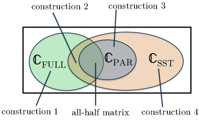
Figure 3: Relations between various models of pairwise comparisons. The constructions proving these relations are presented as a part of the proof of Proposition 5.

The various relationships in Proposition 5 are depicted pictorially in Figure 3. These relations are derived by first establishing certain conditions that matrices in the classes considered must satisfy, and then constructing matrices that satisfy or violate one or more of these conditions. The conditions on $\mathbb{C}_{\mbox{\scalebox{0.5}{{FULL}}}}$ arise from the observation that the class is the convex hull of all SST matrices that have their non-diagonal elements in $\{0,1\}$; we derive conditions on this convex hull that leads to properties of the $\mathbb{C}_{\mbox{\scalebox{0.5}{{FULL}}}}$ class. To handle the parametric class $\mathbb{C}_{\mbox{\scalebox{0.5}{{PAR}}}}$, we employ a necessary condition discussed earlier in Section 2.4 and defined formally in Lemma 12. The SST class $\mathbb{C}_{\mbox{\scalebox{0.5}{{SST}}}}$ is characterized using the insights derived throughout the paper.

D.3 Proof of Proposition 4

We will derive an order one lower bound under the moderate stochastic transitivity condition. This result automatically implies the order one lower bound for weak stochastic transitivity.

The proof imposes a certain structure on a subset of the entries of $M^{*}$ in a manner that $\Theta(n^{2})$ remaining entries are free to take arbitrary values within the interval $[{\frac{1}{2}},1]$. This flexibility then establishes a minimax error of $\Theta(1)$ as claimed.

Let us suppose $M^{*}$ corresponds to the identity permutation of the $n$ items, and that this information is public knowledge. Set the entries of $M^{*}$ above the diagonal in the following manner. For every $i\in[n]$ and every odd $j\in[n]$, set $M^{*}_{ij}={\frac{1}{2}}$. For every $i\in[n]$ and every even $j\in[n]$, set $M^{*}_{ji}={\frac{1}{2}}$. This information is also assumed to be public knowledge. Let $\mathcal{S}\subset[n]^{2}$ denote the set of all entries of $M^{*}$ above the diagonal whose values were not assigned in the previous step. Let $|\mathcal{S}|$ denote the size of set $\mathcal{S}$. The entries below the diagonal are governed by the skew-symmetry constraints.

We first argue that every entry in $\mathcal{S}$ can take arbitrary values in the interval $[{\frac{1}{2}},1]$, and are not constrained by each other under the moderate stochastic transitivity condition. To this end, consider any entry $(i,k)\in\mathcal{S}$. Recall that the moderate stochastic transitivity condition imposes the following set of restrictions in $M^{*}_{ik}$: for every $j$, $M^{*}_{ik}\geq\min\{M^{*}_{ij},M^{*}_{jk}\}$. From our earlier construction we have that for every odd value of $j$, $M^{*}_{ij}={\frac{1}{2}}$ and hence the restriction simply reduces to $M^{*}_{ik}\geq{\frac{1}{2}}$. On the other hand, for every even value of $j$, our construction gives $M^{*}_{jk}={\frac{1}{2}}$, and hence the restriction again reduces to $M^{*}_{ik}\geq{\frac{1}{2}}$. Given the absence of any additional restrictions, the error $\mathbb{E}[|\!|\!|\widehat{M}-M^{*}|\!|\!|_{{\mbox{\tiny{F}}}}^{2}]\geq c|\mathcal{S}|$. Finally, observe that every entry $(i,k)$ where $i<k$, $i$ is odd and $k$ is even belongs to the set $\mathcal{S}$. It follows that $|\mathcal{S}|\geq\frac{n^{2}}{8}$, thus proving our claim.

D.4 Proof of Proposition 5

The constructions governing the claimed relations are enumerated in Figure 3 and the details are provided below.

It is easy to see that since $F$ is non-decreasing, the parametric class $\mathbb{C}_{\mbox{\scalebox{0.5}{{PAR}}}}$ is contained in the strong stochastic transitivity class $\mathbb{C}_{\mbox{\scalebox{0.5}{{SST}}}}$. We provide a formal proof of this statement for the sake of completeness. Suppose without loss of generality that $w_{1}\geq\cdots\geq w_{n}$. Then we claim that the distribution of pairwise comparisons generated through this model result in a matrix, say $M$, that lies in the SST model with the ordering following the identity permutation. This is because for any $i>j>k$,

$$w_{i}-w_{k} \geq w_{i}-w_{j}$$

$$F(w_{i}-w_{k}) \geq F(w_{i}-w_{j})$$

$$M_{ik} \geq M_{ij}.$$

We now show the remaining relations with the four constructions indicated in Figure 3. While these constructions target some specific value of $n$, the results hold for any value $n$ greater than that specific value. To see this, suppose we construct a matrix $M$ for some $n=n_{0}$, and show that it lies inside (or outside) one of these classes. Consider any $n>n_{0}$, and define a $(n\times n)$ matrix $M^{\prime}$ as having $M$ as the top-left $(n_{0}\times n_{0})$ block, ${\frac{1}{2}}$ on the remaining diagonal entries, $1$ on the remaining entries above the diagonal and $0$ on the remaining entries below the diagonal. This matrix $M^{\prime}$ will retain the properties of $M$ in terms of lying inside (or outside, respectively) the claimed class.

In this proof, we use the notation $i\succ j$ to represent a greater preference for $i$ as compared to $j$.

D.4.1 Construction 1

We construct a matrix $M$ such that $M\in\mathbb{C}_{\mbox{\scalebox{0.5}{{FULL}}}}$ but $M\notin\mathbb{C}_{\mbox{\scalebox{0.5}{{SST}}}}$. Let $n=3$. Consider the following distribution over permutations of $3$ items $(1,2,3)$:

$$\mathbb{P}(1\succ 2\succ 3) =\frac{2}{5},$$

$$\mathbb{P}(3\succ 1\succ 2) =\frac{1}{5},$$

$$\mathbb{P}(2\succ 3\succ 1) =\frac{2}{5}.$$

This distribution induces the pairwise marginals

$$\mathbb{P}(1\succ 2) =\frac{3}{5},$$

$$\mathbb{P}(2\succ 3) =\frac{4}{5},$$

$$\mathbb{P}(3\succ 1) =\frac{3}{5}.$$

Set $M_{ij}=\mathbb{P}(i\succ j)$ for every pair. By definition of the class $\mathbb{C}_{\mbox{\scalebox{0.5}{{FULL}}}}$, we have $M\in\mathbb{C}_{\mbox{\scalebox{0.5}{{FULL}}}}$.

A necessary condition for a matrix $M$ to belong to the class $\mathbb{C}_{\mbox{\scalebox{0.5}{{SST}}}}$ is that there must exist at least one item, say item $i$, such that $M_{ij}\geq{\frac{1}{2}}$ for every item $j$. One can verify that the pairwise marginals enumerated above do not satisfy this condition, and hence $M\notin\mathbb{C}_{\mbox{\scalebox{0.5}{{SST}}}}$.

D.4.2 Construction 2

We construct a matrix $M$ such that $M\in\mathbb{C}_{\mbox{\scalebox{0.5}{{SST}}}}\cap\mathbb{C}_{\mbox{\scalebox{0.5}{{FULL}}}}$ but $M\notin\mathbb{C}_{\mbox{\scalebox{0.5}{{PAR}}}}$. Let $n=4$ and consider the following distribution over permutations of $4$ items $(1,2,3,4)$:

$$\mathbb{P}(3\succ 1\succ 2\succ 4)=\frac{1}{8}, \qquad\mathbb{P}(1\succ 2\succ 4\succ 3)=\frac{1}{8}$$

$$\mathbb{P}(2\succ 1\succ 4\succ 3)=\frac{2}{8} \quad\mbox{and}\quad\mathbb{P}(1\succ 2\succ 3\succ 4)=\frac{4}{8}.$$

One can verify that this distribution leads to the following pairwise comparison matrix $M$ (with the ordering of the rows and columns respecting the permutation $1\succ 2\succ 3\succ 4$):

$$M:\,=\frac{1}{8}\begin{bmatrix}4&6&7&8\\ 2&4&7&8\\ 1&1&4&5\\ 0&0&3&4\end{bmatrix}.$$

It is easy to see that this matrix $M\in\mathbb{C}_{\mbox{\scalebox{0.5}{{SST}}}}$, and by construction $M\in\mathbb{C}_{\mbox{\scalebox{0.5}{{FULL}}}}$. Finally, the proof of Proposition 4 shows that $M\notin\mathbb{C}_{\mbox{\scalebox{0.5}{{PAR}}}}$, thereby completing the proof.

D.4.3 Construction 3

We construct a matrix $M$ such that $M\in\mathbb{C}_{\mbox{\scalebox{0.5}{{PAR}}}}$ (and hence $M\in\mathbb{C}_{\mbox{\scalebox{0.5}{{SST}}}}$) but $M\notin\mathbb{C}_{\mbox{\scalebox{0.5}{{FULL}}}}$. First observe that any total ordering on $n$ items can be represented as an $(n\times n)$ matrix in the SST class such that all its off-diagonal entries take values in $\{0,1\}$. The class $\mathbb{C}_{\mbox{\scalebox{0.5}{{FULL}}}}$ is precisely the convex hull of all such binary SST matrices.

Let $B^{1},\ldots,B^{n!}$ denote all $(n\times n)$ matrices in $\mathbb{C}_{\mbox{\scalebox{0.5}{{SST}}}}$ whose off-diagonal elements are restricted to take values in the set $\{0,1\}$. The following lemma derives a property that any matrix in the convex hull of $B^{1},\ldots,B^{n!}$ must satisfy.

Lemma 13.

Consider any $M\in\mathbb{C}_{\mbox{\scalebox{0.5}{{SST}}}}$, and consider three items $i,j,k\in[n]$ such that $M$ respects the ordering $i\succ j\succ k$. Suppose $M_{ij}=M_{jk}={\frac{1}{2}}$ and $M_{ik}=1$. Further suppose that $M$ can be written as

$$M=\sum_{\ell\in[n!]}\alpha^{\ell}B^{\ell},$$ (59)

where $\alpha^{\ell}\geq 0~{}\forall~{}\ell$ and $\sum_{\ell=1}^{n!}\alpha^{\ell}=1$. Then for any $\ell\in[n!]$ such that $\alpha^{\ell}>0$, it must be that $B_{ij}^{\ell}\neq B_{jk}^{\ell}$.

The proof of the lemma is provided at the end of this section.

Now consider the following $(7\times 7)$ matrix $M\in\mathbb{C}_{\mbox{\scalebox{0.5}{{SST}}}}$:

$$M:\,=\left[\begin{array}[]{ccccccc}\pagecolor{black!50}{\frac{1}{2}}&{\frac{1}{2}}&1&1&1&1&1\\ {\frac{1}{2}}&\pagecolor{black!50}{\frac{1}{2}}&{\frac{1}{2}}&{\frac{1}{2}}&1&1&1\\ 0&{\frac{1}{2}}&\pagecolor{black!50}{\frac{1}{2}}&{\frac{1}{2}}&{\frac{1}{2}}&1&1\\ 0&{\frac{1}{2}}&{\frac{1}{2}}&\pagecolor{black!50}{\frac{1}{2}}&{\frac{1}{2}}&{\frac{1}{2}}&1\\ 0&0&{\frac{1}{2}}&{\frac{1}{2}}&\pagecolor{black!50}{\frac{1}{2}}&{\frac{1}{2}}&1\\ 0&0&0&{\frac{1}{2}}&{\frac{1}{2}}&\pagecolor{black!50}{\frac{1}{2}}&{\frac{1}{2}}\\ 0&0&0&0&0&{\frac{1}{2}}&\pagecolor{black!50}{\frac{1}{2}}\end{array}\right].$$ (67)

We will now show via proof by contradiction that $M$ cannot be represented as a convex combination of the matrices $B^{1},\ldots,B^{n!}$. We will then show that $M\in\mathbb{C}_{\mbox{\scalebox{0.5}{{PAR}}}}$.

Suppose one can represent $M$ as a convex combination $M=\sum_{\ell\in[n!]}\alpha^{\ell}B^{\ell}$, where $\alpha^{1},\ldots,\alpha^{n!}$ are non-negative scalars that sum to one. Consider any $\ell$ such that $\alpha^{\ell}\neq 0$. Let $B^{\ell}_{12}=b\in\{0,1\}$. Let us derive some more constraints on $B^{\ell}$. Successively applying Lemma 13 for the following values of $i,j,k$ implies that $B^{\ell}$ must necessarily have the form (75) shown below. Here $\bar{b}:\,=1-b$ and ‘$*$’ denotes some arbitrary value that is irrelevant to the discussion at hand.

• $i=1,j=2,k=3$ gives $B^{\ell}_{23}=\bar{b}$

• $i=1,j=2,k=4$ gives $B^{\ell}_{24}=\bar{b}$

• $i=2,j=3,k=5$ gives $B^{\ell}_{35}={b}$

• $i=2,j=4,k=6$ gives $B^{\ell}_{46}={b}$

• $i=3,j=5,k=6$ gives $B^{\ell}_{56}=\bar{b}$

• $i=4,j=6,k=7$ gives $B^{\ell}_{67}=\bar{b}$.

Thus $B^{\ell}$ must be of the form

$$B^{\ell}=\left[\begin{array}[]{ccccccc}\pagecolor{black!50}{\frac{1}{2}}&b&1&1&1&1&1\\ {\frac{1}{2}}&\pagecolor{black!50}{\frac{1}{2}}&\bar{b}&\bar{b}&1&1&1\\ 0&b&\pagecolor{black!50}{\frac{1}{2}}&*&b&1&1\\ 0&b&*&\pagecolor{black!50}{\frac{1}{2}}&*&b&1\\ 0&0&\bar{b}&*&\pagecolor{black!50}{\frac{1}{2}}&\bar{b}&1\\ 0&0&0&\bar{b}&b&\pagecolor{black!50}{\frac{1}{2}}&\bar{b}\\ 0&0&0&0&0&b&\pagecolor{black!50}{\frac{1}{2}}\end{array}\right].$$ (75)

Finally, applying Lemma 13 with $i=5$, $j=6$ and $k=7$ implies that $B^{\ell}_{67}=b$, which contradicts the necessary condition in equation (75). We have thus shown that $M\notin\mathbb{C}_{\mbox{\scalebox{0.5}{{FULL}}}}$.

We now show that the matrix $M$ constructed in equation (67) is contained in the class $\mathbb{C}_{\mbox{\scalebox{0.5}{{PAR}}}}$. Consider the following function $F:[-1,1]\rightarrow[0,1]$ in the definition of a parametric class:

$$F(x)=\begin{cases}0&\qquad\mbox{if $x<-0.25$}\\ {\frac{1}{2}}&\qquad\mbox{if $-0.25\leq x\leq 0.25$}\\ 1&\qquad\mbox{if $x>0.25$}.\end{cases}$$

Let $n=7$ with $w_{1}=.9$, $w_{2}=.7$, $w_{3}=.6$, $w_{4}=.5$, $w_{5}=.4$, $w_{6}=.3$ and $w_{7}=.1$. One can verify that under this construction, the matrix of pairwise comparisons is identical to that in equation (67).

Proof of Lemma 13

In what follows, we show that $\sum_{\ell:B_{ij}^{\ell}=1,B_{jk}^{\ell}=1}\alpha^{\ell}=\sum_{\ell:B_{ij}^{\ell}=1,B_{jk}^{\ell}=1}\alpha^{\ell}=0$. The result then follows immediately.

Consider some $\ell^{\prime}\in[n!]$ such that $\alpha^{\ell^{\prime}}>0$ and $B_{ij}^{\ell^{\prime}}=0$. Since $M_{ik}=1$, we must have $B_{ik}^{\ell^{\prime}}=1$. Given that $B^{\ell^{\prime}}$ represents a total ordering of the $n$ items, that is, $B^{\ell^{\prime}}$ is an SST matrix with boolean-valued its off-diagonal elements, $B_{ij}^{\ell^{\prime}}=0$ and $B_{ik}^{\ell^{\prime}}=1$ imply that $B_{jk}^{\ell^{\prime}}=1$. We have thus shown that $B_{jk}^{\ell^{\prime}}=1$ whenever $B_{ij}^{\ell^{\prime}}=0$. This result has two consequences. The first consequence is that $\sum_{\ell:B_{ij}^{\ell}=0,B_{jk}^{\ell}=0}\alpha^{\ell}=0$. The second consequence employs the additional fact that $M_{ij}={\frac{1}{2}}$ and hence $\sum_{\ell:B_{ij}^{\ell}=0}\alpha^{\ell}={\frac{1}{2}}$, and then gives $\sum_{\ell:B_{ij}^{\ell}=0,B_{jk}^{\ell}=1}\alpha^{\ell}={\frac{1}{2}}$. Building on, we have

$${\frac{1}{2}}=M_{jk}=\sum_{\ell:B_{ij}^{\ell}=0,B_{jk}^{\ell}=1}\alpha^{\ell}+\sum_{\ell:B_{ij}^{\ell}=1,B_{jk}^{\ell}=1}\alpha^{\ell},$$

and hence we have $\sum_{\ell:B_{ij}^{\ell}=1,B_{jk}^{\ell}=1}\alpha^{\ell}=0$, thus completing the proof.

D.4.4 Construction 4

We construct a matrix $M$ such that $M\in\mathbb{C}_{\mbox{\scalebox{0.5}{{SST}}}}$ but $M\notin\mathbb{C}_{\mbox{\scalebox{0.5}{{FULL}}}}$ and $M\notin\mathbb{C}_{\mbox{\scalebox{0.5}{{PAR}}}}$. Consider $n=11$. Let $M_{2}$ denote the $(4\times 4)$ matrix of Construction 2 and let $M_{3}$ denote the $(7\times 7)$ matrix of construction $3$. Consider the $(11\times 11)$ matrix $M$ of the form

$$M:\,=\begin{bmatrix}M_{2}&1\\ 0&M_{3}\end{bmatrix}.$$

Since $M_{2}\in\mathbb{C}_{\mbox{\scalebox{0.5}{{SST}}}}$ and $M_{3}\in\mathbb{C}_{\mbox{\scalebox{0.5}{{SST}}}}$, it is easy to see that $M\in\mathbb{C}_{\mbox{\scalebox{0.5}{{SST}}}}$. Since $M_{2}\notin\mathbb{C}_{\mbox{\scalebox{0.5}{{PAR}}}}$ and $M\notin\mathbb{C}_{\mbox{\scalebox{0.5}{{FULL}}}}$, it follows that $M\notin\mathbb{C}_{\mbox{\scalebox{0.5}{{PAR}}}}$ and $M\notin\mathbb{C}_{\mbox{\scalebox{0.5}{{FULL}}}}$. This construction completes the proof of Proposition 5.

References

• [ACN08] N. Ailon, M. Charikar, and A. Newman. Aggregating inconsistent information: ranking and clustering. Journal of the ACM (JACM), 55(5):23, 2008.
• [Alo06] N. Alon. Ranking tournaments. SIAM Journal on Discrete Mathematics, 20(1):137–142, 2006.
• [BH11] A. E. Brouwer and W. H. Haemers. Spectra of graphs. Springer, 2011.
• [BM08] M. Braverman and E. Mossel. Noisy sorting without resampling. In Proc. ACM-SIAM symposium on Discrete algorithms, pages 268–276, 2008.
• [BT52] R. A. Bradley and M. E. Terry. Rank analysis of incomplete block designs: I. The method of paired comparisons. Biometrika, pages 324–345, 1952.
• [BW97] T. P. Ballinger and N. T. Wilcox. Decisions, error and heterogeneity. The Economic Journal, 107(443):1090–1105, 1997.
• [Cat12] M. Cattelan. Models for paired comparison data: A review with emphasis on dependent data. Statistical Science, 27(3):412–433, 2012.
• [CGS15] S. Chatterjee, A. Guntuboyina, and B. Sen. On matrix estimation under monotonicity constraints. arXiv:1506.03430, 2015.
• [Cha14] S. Chatterjee. Matrix estimation by universal singular value thresholding. The Annals of Statistics, 43(1):177–214, 2014.
• [CR11] F. Chung and M. Radcliffe. On the spectra of general random graphs. The electronic journal of combinatorics, 18(1):P215, 2011.
• [CS15] Y. Chen and C. Suh. Spectral MLE: Top-$k$ rank aggregation from pairwise comparisons. In International Conference on Machine Learning, 2015.
• [DG77] P. Diaconis and R. L. Graham. Spearman’s footrule as a measure of disarray. Journal of the Royal Statistical Society. Series B (Methodological), pages 262–268, 1977.
• [Dia89] P. Diaconis. A generalization of spectral analysis with application to ranked data. The Annals of Statistics, 17(3):949–979, 1989.
• [DIS15] W. Ding, P. Ishwar, and V. Saligrama. A topic modeling approach to ranking. International Conference on Artificial Intelligence and Statistics, 2015.
• [DM59] D. Davidson and J. Marschak. Experimental tests of a stochastic decision theory. Measurement: Definitions and theories, pages 233–69, 1959.
• [Fis73] P. C. Fishburn. Binary choice probabilities: on the varieties of stochastic transitivity. Journal of Mathematical psychology, 10(4):327–352, 1973.
• [FJS13] V. F. Farias, S. Jagabathula, and D. Shah. A nonparametric approach to modeling choice with limited data. Management Science, 59(2):305–322, 2013.
• [FV93] M. A. Fligner and J. S. Verducci. Probability models and statistical analyses for ranking data, volume 80. Springer, 1993.
• [GD14] M. Gavish and D. L. Donoho. The optimal hard threshold for singular values is. IEEE Transactions on Information Theory, 60(8):5040–5053, 2014.
• [Gil52] E. N. Gilbert. A comparison of signalling alphabets. Bell System Technical Journal, 31(3):504–522, 1952.
• [GW07] F. Gao and J. A. Wellner. Entropy estimate for high-dimensional monotonic functions. Journal of Multivariate Analysis, 98(9):1751–1764, 2007.
• [HOX14] B. Hajek, S. Oh, and J. Xu. Minimax-optimal inference from partial rankings. In Advances in Neural Information Processing Systems, pages 1475–1483, 2014.
• [KMS07] C. Kenyon-Mathieu and W. Schudy. How to rank with few errors. In Symposium on Theory of computing (STOC), pages 95–103. ACM, 2007.
• [KOVB14] T. Kolokolnikov, B. Osting, and J. Von Brecht. Algebraic connectivity of Erdös-Rényi graphs near the connectivity threshold. Available online http://www.mathstat.dal.ca/ tkolokol/papers/braxton-james.pdf, 2014.
• [KR05] T. Klein and E. Rio. Concentration around the mean for maxima of empirical processes. The Annals of Probability, 33(3):1060–1077, 2005.
• [Led01] M. Ledoux. The Concentration of Measure Phenomenon. Mathematical Surveys and Monographs. American Mathematical Society, Providence, RI, 2001.
• [Luc59] R. D. Luce. Individual choice behavior: A theoretical analysis. New York: Wiley, 1959.
• [Mar96] J. I. Marden. Analyzing and modeling rank data. CRC Press, 1996.
• [ML65] D. H. McLaughlin and R. D. Luce. Stochastic transitivity and cancellation of preferences between bitter-sweet solutions. Psychonomic Science, 2(1-12):89–90, 1965.
• [NOS12] S. Negahban, S. Oh, and D. Shah. Iterative ranking from pair-wise comparisons. In Advances in Neural Information Processing Systems, pages 2474–2482, 2012.
• [Oli09] R. I. Oliveira. Concentration of the adjacency matrix and of the Laplacian in random graphs with independent edges. arXiv preprint:0911.0600, 2009.
• [RA14] A. Rajkumar and S. Agarwal. A statistical convergence perspective of algorithms for rank aggregation from pairwise data. In International Conference on Machine Learning, pages 118–126, 2014.
• [Sam00] P.-M. Samson. Concentration of measure inequalities for Markov chains and $\phi$-mixing processes. Annals of Probability, pages 416–461, 2000.
• [SBB+16] N. B. Shah, S. Balakrishnan, J. Bradley, A. Parekh, K. Ramchandran, and M. J. Wainwright. Estimation from pairwise comparisons: Sharp minimax bounds with topology dependence. Journal of Machine Learning Research, 17(58):1–47, 2016.
• [SBW16] N. B. Shah, S. Balakrishnan, and M. J. Wainwright. Feeling the Bern: Adaptive estimators for Bernoulli probabilities of pairwise comparisons. arXiv preprint arXiv:1603.06881, 2016.
• [SS11] M. J. Silvapulle and P. K. Sen. Constrained statistical inference: Order, inequality, and shape constraints, volume 912. John Wiley & Sons, 2011.
• [Tao12] T. Tao. Topics in random matrix theory, volume 132. American Mathematical Society Providence, RI, 2012.
• [Tho76] R. Thompson. The behavior of eigenvalues and singular values under perturbations of restricted rank. Linear Algebra and its Applications, 13(1):69–78, 1976.
• [Thu27] L. L. Thurstone. A law of comparative judgment. Psychological Review, 34(4):273, 1927.
• [Tve72] A. Tversky. Elimination by aspects: A theory of choice. Psychological review, 79(4):281, 1972.
• [Var57] R. Varshamov. Estimate of the number of signals in error correcting codes. In Dokl. Akad. Nauk SSSR, volume 117, pages 739–741, 1957.
• [VDVW96] A. Van Der Vaart and J. Wellner. Weak convergence. In Weak Convergence and Empirical Processes, pages 16–28. Springer, 1996.
• [WJJ13] F. L. Wauthier, M. I. Jordan, and N. Jojic. Efficient ranking from pairwise comparisons. In Proceedings of the 30th International Conference on Machine Learning (ICML), 2013.