Optimization for Gaussian Processes via Chaining

Emile Contal CMLA, UMR CNRS 8536, ENS Cachan Cédric Malherbe CMLA, UMR CNRS 8536, ENS Cachan Nicolas Vayatis CMLA, UMR CNRS 8536, ENS Cachan
Abstract

In this paper, we consider the problem of stochastic optimization under a bandit feedback model. We generalize the GP-UCB algorithm [Srinivas and al., 2012] to arbitrary kernels and search spaces. To do so, we use a notion of localized chaining to control the supremum of a Gaussian process, and provide a novel optimization scheme based on the computation of covering numbers. The theoretical bounds we obtain on the cumulative regret are more generic and present the same convergence rates as the GP-UCB algorithm. Finally, the algorithm is shown to be empirically more efficient than its natural competitors on simple and complex input spaces.

1 Introduction

Optimizing an unknown and noisy function is at the center of many applications in the field of machine learning [1]. The goal of a sequential optimization procedure may be either seen as maximizing the sum of the outputs (or rewards) received at each iteration, that is to minimize the cumulative regret widely used in bandit problems, or as maximizing the best reward received so far, that is to minimize the simple regret. This task becomes challenging when we only have mild information about the unknown function. To tackle this challenge, a Bayesian approach has been shown to be empirically efficient [2, 3, 4, 5, 6]. In this approach, we model the unknown function as a realization of a Gaussian Process (GP) which allows to control the assumptions we put on the smoothness of the function by choosing different kernels [7]. In order to prove theoretical guarantees on the regret, algorithms in the literature typically rely on high probabilistic upper confidence bounds (UCB) [8, 9, 10, 11, 12]. In these works and many others, the UCB is obtained with a union bound over all the points of a discretization of the input space. The major drawback of this approach is that the UCB depends on the cardinality of the discretization instead of the complexity of the input space itself. As a consequence, the convergence rates derived on the regret become arbitrary large when the discretization becomes finer and finer. Aiming at filling this gap between theory and practice we propose an efficient computation of chaining for Bayesian Optimization. Chaining, that has been recently studied in the context of sequential optimization (see [13] for bandit with known horizon or [14] in the case of online regression), appears to be an ideal tool to capture the complexity of the search space with respect to the smoothness of the function. The contribution of this paper is twofold: we first introduce a novel policy based on the computation of covering numbers called the Chaining-UCB that can be seen as a generalization of the GP-UCB algorithm with automatic calibration of the exploration/exploitation tradeoff for arbitrary kernels and search space. On the other hand, we provide theoretical guarantees on its regret with the same convergence rates as its competitors, without depending on the cardinality of the discretization of the search space. The rest of the paper is organized as follows: in Section 2, we present the framework of our analysis, the basic properties of GP and we introduce the Chaining-UCB algorithm. In Section 3, we present and discuss the upper bound on the regret. Finally in Section 4 we compare the empirical performances 111The MATLAB code is available on http://econtal.perso.math.cnrs.fr/software/ of the Chaining-UCB algorithm to its natural competitors on simple input spaces, that is Dsuperscript𝐷\mathbb{R}^{D}, and complex input spaces, this is directed graphs space.

for t=1,2,𝑡12italic-…t=1,2,\dots do
       Compute μtsubscript𝜇𝑡\mu_{t}, σtsubscript𝜎𝑡\sigma_{t} and dtsubscript𝑑𝑡d_{t}
       T0subscript𝑇0T_{0}\leftarrow\emptyset; σtmin=minx𝒳σt(x)superscriptsubscript𝜎𝑡minsubscript𝑥𝒳subscript𝜎𝑡𝑥\sigma_{t}^{\text{min}}=\min_{x\in\mathcal{X}}\sigma_{t}(x)
       for i=11log2(σtmin)𝑖11subscript2superscriptsubscript𝜎𝑡mini=1\dots\lceil 1-\log_{2}(\sigma_{t}^{\text{min}})\rceil do
             ϵi2i+1subscriptitalic-ϵ𝑖superscript2𝑖1\epsilon_{i}\leftarrow 2^{-i+1}
             𝒳¯{x𝒳:dt(x,Ti1)>ϵi}¯𝒳conditional-set𝑥𝒳subscript𝑑𝑡𝑥subscript𝑇𝑖1subscriptitalic-ϵ𝑖\bar{\mathcal{X}}\leftarrow\{x\in\mathcal{X}:d_{t}(x,T_{i-1})>\epsilon_{i}\}
             TiTi1Cover(𝒳¯,dt,ϵi)subscript𝑇𝑖subscript𝑇𝑖1Cover¯𝒳subscript𝑑𝑡subscriptitalic-ϵ𝑖T_{i}\leftarrow T_{i-1}\cup\textsc{Cover}(\bar{\mathcal{X}},d_{t},\epsilon_{i})
             Hiϵi2log((|Ti|+1)i2t2π4δ62)subscript𝐻𝑖subscriptitalic-ϵ𝑖2subscript𝑇𝑖1superscript𝑖2superscript𝑡2superscript𝜋4𝛿superscript62H_{i}\leftarrow\epsilon_{i}\sqrt{2\log\Big{(}(\left\lvert T_{i}\right\rvert+1)i^{2}t^{2}\frac{\pi^{4}}{\delta 6^{2}}\Big{)}}
            
       end for
      xtargmaxx𝒳μt(x)+i:σtminϵi<σt(x)Hisubscript𝑥𝑡subscript𝑥𝒳subscript𝜇𝑡𝑥subscript:𝑖superscriptsubscript𝜎𝑡minsubscriptitalic-ϵ𝑖subscript𝜎𝑡𝑥subscript𝐻𝑖\displaystyle x_{t}\leftarrow\operatorname*{\arg\!\max}_{x\in\mathcal{X}}\mu_{t}(x)+\sum_{i:\sigma_{t}^{\text{min}}\leq\epsilon_{i}<\sigma_{t}(x)}H_{i}
       Sample xtsubscript𝑥𝑡x_{t} and observe ytsubscript𝑦𝑡y_{t}
      
end for
Algorithm 1 Chaining-UCB(𝒳,k(,),η𝒳𝑘𝜂\mathcal{X},k(\cdot,\cdot),\eta)
T𝑇T\leftarrow\emptyset; 𝒳¯𝒳¯𝒳𝒳\bar{\mathcal{X}}\leftarrow\mathcal{X}
x,x𝒳,G[x,x]𝟙d(x,x)ϵformulae-sequencefor-all𝑥superscript𝑥𝒳𝐺𝑥superscript𝑥subscript1𝑑𝑥superscript𝑥italic-ϵ\forall x,x^{\prime}\in\mathcal{X},~{}G[x,x^{\prime}]\leftarrow\mathds{1}_{d(x,x^{\prime})\leq\epsilon}
while 𝒳¯¯𝒳\bar{\mathcal{X}}\neq\emptyset do
       xargmaxx𝒳¯x𝒳¯G[x,x]𝑥subscript𝑥¯𝒳subscriptsuperscript𝑥¯𝒳𝐺𝑥superscript𝑥x\leftarrow\operatorname*{\arg\!\max}_{x\in\bar{\mathcal{X}}}\sum_{x^{\prime}\in\bar{\mathcal{X}}}G[x,x^{\prime}]
       TT{x}𝑇𝑇𝑥\displaystyle T\leftarrow T\cup\{x\}
       𝒳¯𝒳¯{x𝒳¯:G[x,x]=1}¯𝒳¯𝒳conditional-setsuperscript𝑥¯𝒳𝐺𝑥superscript𝑥1\bar{\mathcal{X}}\leftarrow\bar{\mathcal{X}}\setminus\{x^{\prime}\in\bar{\mathcal{X}}:G[x,x^{\prime}]=1\}
      
end while
return T𝑇T
Algorithm 2 Greedy-Cover(𝒳,d,ϵ)𝒳𝑑italic-ϵ(\mathcal{X},d,\epsilon)

2 The Chaining-UCB algorithm

Bayesian optimization framework.

Let f:𝒳:𝑓𝒳f:\mathcal{X}\to\mathbb{R} be the unknown function we want to optimize, where 𝒳𝒳\mathcal{X} is the input space which is not necessarily a subset of Dsuperscript𝐷\mathbb{R}^{D}. We assume that f𝑓f is a realization of a centered Gaussian process with known kernel k𝑘k satisfying k(x,x)1𝑘𝑥superscript𝑥1k(x,x^{\prime})\leq 1 for all (x,x)𝒳2𝑥superscript𝑥superscript𝒳2(x,x^{\prime})\in\mathcal{X}^{2}. To avoid measurability issues we suppose that 𝒳𝒳\mathcal{X} is a finite set with arbitrary cardinality (see [15, 16] for more details). A sequential optimization algorithm iterates two steps: it first chooses xnsubscript𝑥𝑛x_{n} based on y1,,yn1subscript𝑦1subscript𝑦𝑛1y_{1},\dots,y_{n-1}, and next gets the noisy observation yn=f(xn)+ϵnsubscript𝑦𝑛𝑓subscript𝑥𝑛subscriptitalic-ϵ𝑛y_{n}=f(x_{n})+\epsilon_{n} where (ϵn)n1subscriptsubscriptitalic-ϵ𝑛𝑛1(\epsilon_{n})_{n\geq 1} are independent Gaussians 𝒩(0,η2)𝒩0superscript𝜂2\mathcal{N}(0,\eta^{2}) with known variance η2superscript𝜂2\eta^{2}. Let Xn={x1,,xn}subscript𝑋𝑛subscript𝑥1subscript𝑥𝑛X_{n}=\{x_{1},\dots,x_{n}\} be the set of queried points after n𝑛n iterations and 𝐘n=[y1,,yn]subscript𝐘𝑛subscript𝑦1subscript𝑦𝑛\mathbf{Y}_{n}=[y_{1},\dots,y_{n}] the associated observations packed in vector form. Unlike the work of [13] this paper considers that the time horizon n𝑛n is unknown. For GP, the distribution of f𝑓f conditioned on 𝐘nsubscript𝐘𝑛\mathbf{Y}_{n} is a non-centered GP of mean μn+1subscript𝜇𝑛1\mu_{n+1} and kernel kn+1subscript𝑘𝑛1k_{n+1} computed as follows for all (x,x)𝒳2𝑥superscript𝑥superscript𝒳2(x,x^{\prime})\in\mathcal{X}^{2}:

μn+1(x)=𝐤n(x)𝐂n1𝐘n and kn+1(x,x)=k(x,x)𝐤n(x)𝐂n1𝐤n(x),subscript𝜇𝑛1𝑥subscript𝐤𝑛superscript𝑥topsuperscriptsubscript𝐂𝑛1subscript𝐘𝑛 and subscript𝑘𝑛1𝑥superscript𝑥𝑘𝑥superscript𝑥subscript𝐤𝑛superscript𝑥topsuperscriptsubscript𝐂𝑛1subscript𝐤𝑛superscript𝑥\mu_{n+1}(x)=\mathbf{k}_{n}(x)^{\top}\mathbf{C}_{n}^{-1}\mathbf{Y}_{n}\text{ ~{}and~{} }k_{n+1}(x,x^{\prime})=k(x,x^{\prime})-\mathbf{k}_{n}(x)^{\top}\mathbf{C}_{n}^{-1}\mathbf{k}_{n}(x^{\prime})\,, (1)

where 𝐤n(x)=[k(xt,x)]xtXnsubscript𝐤𝑛𝑥subscriptdelimited-[]𝑘subscript𝑥𝑡𝑥subscript𝑥𝑡subscript𝑋𝑛\mathbf{k}_{n}(x)=[k(x_{t},x)]_{x_{t}\in X_{n}} is the kernel vector between x𝑥x and Xnsubscript𝑋𝑛X_{n}, and 𝐂n=𝐊n+η2𝐈subscript𝐂𝑛subscript𝐊𝑛superscript𝜂2𝐈\mathbf{C}_{n}=\mathbf{K}_{n}+\eta^{2}\mathbf{I} with 𝐊n=[k(xt,xt)]xt,xtXnsubscript𝐊𝑛subscriptdelimited-[]𝑘subscript𝑥𝑡subscript𝑥superscript𝑡subscript𝑥𝑡subscript𝑥superscript𝑡subscript𝑋𝑛\mathbf{K}_{n}=[k(x_{t},x_{t^{\prime}})]_{x_{t},x_{t^{\prime}}\in X_{n}} the kernel matrix [7]. We also define the variance σn2(x)=kn(x,x)superscriptsubscript𝜎𝑛2𝑥subscript𝑘𝑛𝑥𝑥\sigma_{n}^{2}(x)=k_{n}(x,x) and the pseudo-distance dn(x,x)subscript𝑑𝑛𝑥superscript𝑥d_{n}(x,x^{\star}) :

dn(x,x)=σn2(x)2kn(x,x)+σn2(x).subscript𝑑𝑛𝑥superscript𝑥superscriptsubscript𝜎𝑛2superscript𝑥2subscript𝑘𝑛𝑥superscript𝑥superscriptsubscript𝜎𝑛2𝑥d_{n}(x,x^{\star})=\sqrt{\sigma_{n}^{2}(x^{\star})-2k_{n}(x,x^{\star})+\sigma_{n}^{2}(x)}\,. (2)

Note that dn2(x,x)=Var[f(x)f(x)|Xn,𝐘n]superscriptsubscript𝑑𝑛2𝑥superscript𝑥Vardelimited-[]𝑓superscript𝑥conditional𝑓𝑥subscript𝑋𝑛subscript𝐘𝑛d_{n}^{2}(x,x^{\star})=\mathrm{Var}[f(x^{\star})-f(x)\,|\,X_{n},\mathbf{Y}_{n}]. To measure the complexity of 𝒳𝒳\mathcal{X} we will compute covering numbers with respect to dnsubscript𝑑𝑛d_{n}.

An upper confidence bound algorithm via chaining.

At the core of our strategy to control the regret of the algorithm we need an upper confidence bound (UCB) on supx𝒳f(x)f(x)subscriptsupremumsuperscript𝑥𝒳𝑓superscript𝑥𝑓𝑥\sup_{x^{\star}\in\mathcal{X}}f(x^{\star})-f(x) for all x𝒳𝑥𝒳x\in\mathcal{X}. A naive approach uses a union bound on 𝒳𝒳\mathcal{X}, resulting in a factor log|𝒳|𝒳\sqrt{\log\left\lvert\mathcal{X}\right\rvert} in the UCB, which is not appropriate when 𝒳𝒳\mathcal{X} is a numerical discretization of a continuous space, typically a multi-dimensional grid of high density. We use the chaining trick [17, 18, 19] to get a UCB relying on the covering numbers of 𝒳𝒳\mathcal{X} with respect to dnsubscript𝑑𝑛d_{n} instead of its cardinality. In that way the algorithm adapts to arbitrary input spaces. The main element of our algorithm is the computation of hierarchical ϵitalic-ϵ\epsilon-covers of 𝒳𝒳\mathcal{X}. We say that a subset T𝑇T is an ϵitalic-ϵ\epsilon-cover of 𝒳𝒳\mathcal{X} when for all x𝒳𝑥𝒳x\in\mathcal{X}, dn(x,T)ϵsubscript𝑑𝑛𝑥𝑇italic-ϵd_{n}(x,T)\leq\epsilon, where dn(x,T)=infxTdn(x,x)subscript𝑑𝑛𝑥𝑇subscriptinfimumsuperscript𝑥𝑇subscript𝑑𝑛𝑥superscript𝑥d_{n}(x,T)=\inf_{x^{\prime}\in T}d_{n}(x,x^{\prime}). The covering numbers N(𝒳,dn,ϵ)𝑁𝒳subscript𝑑𝑛italic-ϵN(\mathcal{X},d_{n},\epsilon) are the cardinality of the smallest ϵitalic-ϵ\epsilon-cover of 𝒳𝒳\mathcal{X} for the pseudo-distance dnsubscript𝑑𝑛d_{n}, and the function Cover(𝒳,dn,ϵ𝒳subscript𝑑𝑛italic-ϵ\mathcal{X},d_{n},\epsilon) in Algorithm 1 returns such a set. The Chaining-UCB algorithm then queries the objective function at the point maximizing the UCB obtained by chaining. The computation of an optimal ϵitalic-ϵ\epsilon-cover is \NP-hard, but we can easily build an efficient approximation as shown in Algorithm 2 and discussed in Section 4.

3 Main results

Guarantees on the regret.

In the following theorem we provide a high probabilistic upper bound on the instantaneous regret incurred by Algorithm 1 in terms of the posterior deviations σn(xn)subscript𝜎𝑛subscript𝑥𝑛\sigma_{n}(x_{n}) and covering numbers. This inequality is used in the subsequent corollary to obtain upper bounds on its cumulative and simple regrets.

Theorem 1.

For any finite 𝒳𝒳\mathcal{X}, let x1,x2,subscript𝑥1subscript𝑥2italic-…x_{1},x_{2},\dots be the queries of the Chaining-UCB algorithm on f𝑓f sampled from a 𝒢𝒫(0,k)𝒢𝒫0𝑘\mathcal{GP}(0,k) where k(,)1𝑘1k(\cdot,\cdot)\!\leq\!1. For δ(0,1)𝛿01\delta\in(0,1), using the notations σn=σn(xn)subscript𝜎𝑛subscript𝜎𝑛subscript𝑥𝑛\sigma_{n}=\sigma_{n}(x_{n}) and cn,δ=6logn2π436δ+15subscript𝑐𝑛𝛿6superscript𝑛2superscript𝜋436𝛿15c_{n,\delta}=6\sqrt{\log\frac{n^{2}\pi^{4}}{36\delta}}+15, we have with probability at least 1δ1𝛿1-\delta that for all n𝑛superscriptn\in\mathbb{N}^{\star}:

supx𝒳f(x)f(xn)σn(cn,δ6logσn)+9i:2i<σn2ilogN(𝒳,dn,2i).subscriptsupremumsuperscript𝑥𝒳𝑓superscript𝑥𝑓subscript𝑥𝑛subscript𝜎𝑛subscript𝑐𝑛𝛿6subscript𝜎𝑛9subscript:𝑖superscript2𝑖subscript𝜎𝑛superscript2𝑖𝑁𝒳subscript𝑑𝑛superscript2𝑖\sup_{x^{\star}\in\mathcal{X}}f(x^{\star})-f(x_{n})\leq\sigma_{n}\big{(}c_{n,\delta}-6\log\sigma_{n}\big{)}+9\sum_{i:2^{-i}<\sigma_{n}}2^{-i}\sqrt{\log N(\mathcal{X},d_{n},2^{-i})}\,.

In order to simplify this inequality and get convergence rates for the cumulative regret Rnsubscript𝑅𝑛R_{n} and simple regret Snsubscript𝑆𝑛S_{n}, it is necessary to add some assumptions on k𝑘k and 𝒳𝒳\mathcal{X}. Corollary 1 gives an example of the rates we obtain for the usual Squared-Exponential kernel k(x,x)=e12xx22𝑘𝑥superscript𝑥superscript𝑒12superscriptsubscriptdelimited-∥∥𝑥superscript𝑥22k(x,x^{\prime})=e^{-\frac{1}{2}\smash{\left\lVert x-x^{\prime}\right\rVert_{2}^{2}}} and 𝒳𝒳\mathcal{X} in Dsuperscript𝐷\mathbb{R}^{D}.

Corollary 1.

For the SE kernel and a compact 𝒳[0,R]D𝒳superscript0𝑅𝐷\mathcal{X}\subseteq[0,R]^{D}, the Chaining-UCB algorithm returns a sequence x1,x2,subscript𝑥1subscript𝑥2x_{1},x_{2},\ldots such that Rn=𝒪(n(logn)D+2)subscript𝑅𝑛𝒪𝑛superscript𝑛𝐷2R_{n}=\mathcal{O}\Big{(}\sqrt{n(\log n)^{D+2}}\Big{)} and Sn=𝒪((logn)D+2n)subscript𝑆𝑛𝒪superscript𝑛𝐷2𝑛S_{n}=\mathcal{O}\Big{(}\sqrt{\frac{(\log n)^{D+2}}{n}}\Big{)}.

The proof of Theorem 1 employs the chaining trick to get a local control on the supremum of a non-centered GP. Since this requires to define additional structures, the proofs are postponed to Appendix A. The proof of Corollary 1, in Appendix B, first uses an upper bound on the covering numbers via the Lipschitz property of the SE kernel. It then applies the inequality about the mutual information proven in Theorem 5 of [9] to obtain the given regret rates. It is straightforward to apply this technique to other cases like linear kernels or Matérn kernels with parameter ν>2𝜈2\nu>2, since both the covering numbers and the mutual information can be bounded by similar techniques.
Refer to caption
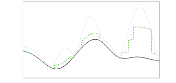
Figure 1: Illustration of the exploration/exploitation tradeoff maximized in Algorithm 1. The red crosses are the noisy observations. The plain black line is the posterior mean μ𝜇\mu. The dashed green line is the target of the Chaining-UCB algorithm. The dotted blue line is the target used by the GP-UCB algorithm. Remark that the rectangular form is explained by the discrete sum.

A flexible algorithm.

A reader familiar with classical chaining may ask why we use the bad-looking sum i:ϵi<σnϵilogN(𝒳,dn,ϵi)subscript:𝑖subscriptitalic-ϵ𝑖subscript𝜎𝑛subscriptitalic-ϵ𝑖𝑁𝒳subscript𝑑𝑛subscriptitalic-ϵ𝑖\sum_{i:\epsilon_{i}<\sigma_{n}}\epsilon_{i}\sqrt{\log N(\mathcal{X},d_{n},\epsilon_{i})} instead of the Dudley integral. Even if the Dudley integral is simple to bound for certain kernel k𝑘k and space 𝒳𝒳\mathcal{X}, we want Algorithm 1 to be able to adapt to all search space without having to tune its parameters. By computing the successive covering numbers, the Chaining-UCB algorithm calibrates automatically the exploration-exploitation tradeoff. This fact contrasts with previous algorithms like GP-UCB where the input parameter βtsubscript𝛽𝑡\beta_{t} depends either on the cardinality |𝒳|𝒳\left\lvert\mathcal{X}\right\rvert or on the Lipschitz constants of the kernel (see Theorems 1 and 2 of [9]). On the computational side, the discrete sum limits the number of ϵisubscriptitalic-ϵ𝑖\epsilon_{i}-covers which need to be computed to only the ϵisubscriptitalic-ϵ𝑖\epsilon_{i} such that ϵi>minx𝒳σn(x)subscriptitalic-ϵ𝑖subscript𝑥𝒳subscript𝜎𝑛𝑥\epsilon_{i}>\min_{x\in\mathcal{X}}\sigma_{n}(x). Thanks to their geometrical decay, these numbers remain low in practice. Figure 1 illustrates the exploration/exploitation tradeoff we obtain with this discrete sum on a 1D toy example, compared to the tradeoff computed with a union bound as in GP-UCB. In Figure 1 a constant term is subtracted from the UCB in order to set the minimum of the exploration terms to zero in both Chaining-UCB and GP-UCB.

4 Practical considerations and experiments

Computing the ϵitalic-ϵ\epsilon-covers efficiently.

As mentioned previously the computation of an optimal ϵitalic-ϵ\epsilon-cover is \NP-hard. We demonstrate here how to build in practice a near-optimal ϵitalic-ϵ\epsilon-cover using a greedy algorithm on graph. First, remark that for any fixed ϵitalic-ϵ\epsilon we can define a graph 𝒢𝒢\mathcal{G} where the nodes are the elements of 𝒳𝒳\mathcal{X} and there is an edge between x𝑥x and xsuperscript𝑥x^{\prime} if and only if d(x,x)ϵ𝑑𝑥superscript𝑥italic-ϵd(x,x^{\prime})\leq\epsilon. The size of this construction is 𝒪(|𝒳|2)𝒪superscript𝒳2\mathcal{O}(\left\lvert\mathcal{X}\right\rvert^{2}). The sparse structure of the underlying graph can be exploited to get an efficient representation. The problem of finding an optimal ϵitalic-ϵ\epsilon-cover reduces to the problem of finding a minimal dominating set on 𝒢𝒢\mathcal{G}. We can therefore use the greedy Algorithm 2 which enjoys an approximation factor of logdmax(𝒢)subscript𝑑max𝒢\log d_{\mathrm{max}}(\mathcal{G}), where dmax(𝒢)subscript𝑑max𝒢d_{\mathrm{max}}(\mathcal{G}) is the maximum degree of 𝒢𝒢\mathcal{G} (see for example [20] for a proof of \NP-hardness and approximation results). This construction leads to an additional (almost constant) term of loglogdmax(𝒢)subscript𝑑max𝒢\sqrt{\log\log d_{\mathrm{max}}(\mathcal{G})} in the right-hand side of Theorem 1. Finally, note that this approximation is optimal unless =\NP\NP\P=\NP as shown in [21].

Refer to caption
(a) SE kernel
Refer to caption
(b) Himmelblau
Refer to caption
(c) Graph kernel
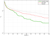
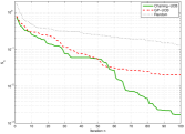
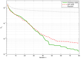
Figure 2: Empirical mean of the simple regret Snsubscript𝑆𝑛S_{n} in terms of iteration n𝑛n for Chaining-UCB, GP-UCB and Random search (lower is better).

Experiments.

In this section we compare the ability of the Chaining-UCB algorithm to find the maximum of an unknown function against the GP-UCB algorithm from [9] and the Random search. For both the Chaining-UCB and the GP-UCB algorithms the value for δ𝛿\delta was set to 0.050.050.05. The Random approach selects the next query uniformly among the unknown locations. It gives a baseline to grasp the scale of the performances of both algorithms. All three strategies are initialized with a set of 101010 noisy observations sampled uniformly over 𝒳𝒳\mathcal{X}. Figure 2 shows the empirical mean of the simple regret Snsubscript𝑆𝑛S_{n} over 32 runs. In every experiments the standard deviation of the noise was set to 0.050.050.05 and the search space is discrete with |𝒳|=104𝒳superscript104\left\lvert\mathcal{X}\right\rvert=10^{4}. The SE experiment consists in generating GPs drawn from a two dimensional isotropic SE kernel, with the kernel bandwidth set to 111. The search space is a uniform design in a square of length 202020. The Himmelblau experiment is a two dimensional polynomial function based on the Himmelblau’s function with the addition of a linear trend. It possesses several local maxima which makes the global optimization challenging. The kernel used by the algorithm is an isotropic SE kernel with the bandwidth chosen by maximizing the marginal likelihood of a subset of training points. Finally we consider the task of optimizing over graphs. Global optimization of graphs can model complex problems as in industrial design, network analysis or computational biology. The input space is the set of directed graphs with less than 202020 nodes. The kernel is the shortest-path kernel [22] normalized such that k(g,g)=1𝑘𝑔𝑔1k(g,g)=1 for g𝒳𝑔𝒳g\in\mathcal{X}. Note that in this synthetic assessment we do not address the question faced in practice of choosing the prior. We further mention that the kernel matrix can be efficiently computed by pre-processing all pairs of shortest paths for each graph with Floyd-Warshall’s algorithm. Figure 2 shows the Chaining-UCB algorithm is empirically more efficient than the GP-UCB algorithm on the three test cases. We remark that in practice, unlike GP-UCB, we may use a design with |𝒳|104much-greater-than𝒳superscript104\left\lvert\mathcal{X}\right\rvert\gg 10^{4} without affecting the performance of Chaining-UCB. However generating a GP costs 𝒪(|𝒳|3)𝒪superscript𝒳3\mathcal{O}(\left\lvert\mathcal{X}\right\rvert^{3}) which limits the tractability of synthetic assessments.

Conclusion.

The theorem we derived and the experiment we performed suggest that the automatic calibration of the exploration/exploitation tradeoff by the hierarchical ϵitalic-ϵ\epsilon-covers effectively adapts to various settings. This chaining approach is a promising step toward generic, sound and tractable algorithms for Bayesian optimization.

References

  • [1] J. Snoek, H. Larochelle, and R. P. Adams. Practical bayesian optimization of machine learning algorithms. In Advances in Neural Information Processing Systems 25, pages 2960–2968, 2012.
  • [2] J. Mockus. Bayesian approach to global optimization. Mathematics and its applications. Kluwer Academic, 1989.
  • [3] D. R. Jones, M. Schonlau, and W. J. Welch. Efficient global optimization of expensive black-box functions. Journal of Global Optimization, 13(4):455–492, December 1998.
  • [4] M. Osborne. Bayesian Gaussian processes for sequential prediction, optimisation and quadrature. PhD thesis, Oxford University New College, 2010.
  • [5] P. Hennig and C. J. Schuler. Entropy search for information-efficient global optimization. Journal of Machine Learning Research, 13:1809–1837, 2012.
  • [6] E. Contal, V. Perchet, and N. Vayatis. Gaussian process optimization with mutual information. In Proceedings of the 31st International Conference on Machine Learning (ICML-14), pages 253–261, 2014.
  • [7] C. E. Rasmussen and C. Williams. Gaussian Processes for Machine Learning. MIT Press, 2006.
  • [8] A. Krause and C.S. Ong. Contextual Gaussian process bandit optimization. In Advances in Neural Information Processing Systems 24, pages 2447–2455, 2011.
  • [9] N. Srinivas, A. Krause, S. Kakade, and M. Seeger. Information-theoretic regret bounds for Gaussian process optimization in the bandit setting. IEEE Transactions on Information Theory, 58(5):3250–3265, 2012.
  • [10] N. de Freitas, A. J. Smola, and M. Zoghi. Exponential regret bounds for Gaussian process bandits with deterministic observations. In Proceedings of the 29th International Conference on Machine Learning. icml.cc / Omnipress, 2012.
  • [11] E. Contal, D. Buffoni, A. Robicquet, and N. Vayatis. Parallel Gaussian process optimization with upper confidence bound and pure exploration. In Machine Learning and Knowledge Discovery in Databases (ECML), volume 8188, pages 225–240. Springer Berlin Heidelberg, 2013.
  • [12] J. Djolonga, A. Krause, and V. Cevher. High-dimensional gaussian process bandits. In Advances in Neural Information Processing Systems, pages 1025–1033, 2013.
  • [13] S. Grunewalder, J-Y. Audibert, M. Opper, and J. Shawe-Taylor. Regret bounds for Gaussian process bandit problems. In Proceedings of the International Conference on Artificial Intelligence and Statistics, pages 273–280. MIT Press, 2010.
  • [14] P. Gaillard and S. Gerchinovitz. A chaining algorithm for online nonparametric regression. Proceedings of the Conference on Learning Theory (COLT), 2015.
  • [15] S. Boucheron, G. Lugosi, and P. Massart. Concentration inequalities: A nonasymptotic theory of independence. Oxford University Press, 2013.
  • [16] E. Giné and R. Nickl. Mathematical foundations of infinite-dimensional statistical models, 2015.
  • [17] M. Talagrand. Upper and Lower Bounds for Stochastic Processes: Modern Methods and Classical Problems, volume 60. Springer-Verlag Berlin Heidelberg, 2014.
  • [18] D. Pollard. Empirical processes: Theory and applications. NSF-CBMS Regional Conference Series in Probability and Statistics, 2:pp. i–iii+v+vii–viii+1–86, 1990.
  • [19] R.M. Dudley. The sizes of compact subsets of hilbert space and continuity of gaussian processes. Journal of Functional Analysis, 1(3):290–330, 1967.
  • [20] David S Johnson. Approximation algorithms for combinatorial problems. In Proceedings of the fifth annual ACM symposium on Theory of computing, pages 38–49. ACM, 1973.
  • [21] R. Raz and S. Safra. A sub-constant error-probability low-degree test, and a sub-constant error-probability pcp characterization of np. In Proceedings of the twenty-ninth annual ACM symposium on Theory of computing, pages 475–484. ACM, 1997.
  • [22] Karsten M Borgwardt and Hans-Peter Kriegel. Shortest-path kernels on graphs. In Data Mining, Fifth IEEE International Conference on, pages 8–pp. IEEE, 2005.

Appendix A Proof of Theorem 1

In this section, we first demonstrate how chaining is used to analyze the supremum of a centered GP. Since our aim is to derive an efficient algorithm, we put some effort to keep low values for the constants. The next subsection shows how this simply extends to non-centered GP and how to build the UCB algorithm with the chaining bound. Finally we express the upper bounds in terms of the covering numbers of 𝒳𝒳\mathcal{X}.

A.1 Using covering trees to bound the supremum of a GP

Let us fix an iteration n𝑛n and the observations 𝐘n1subscript𝐘𝑛1\mathbf{Y}_{n-1}, we define fnsubscript𝑓𝑛f_{n} the centered posterior of f𝑓f conditioned on 𝐘n1subscript𝐘𝑛1\mathbf{Y}_{n-1}, which is a Gaussian process 𝒢𝒫(0,kn)𝒢𝒫0subscript𝑘𝑛\mathcal{GP}(0,k_{n}) where knsubscript𝑘𝑛k_{n} is defined in Equation 1. By Cramer-Chernoff’s method [15] we have for all x,x𝒳superscript𝑥𝑥𝒳x^{\star},x\in\mathcal{X} and u>0𝑢0u>0 that:

Pr[fn(x)fn(x)>dn(x,x)2u]<eu,Prsubscript𝑓𝑛superscript𝑥subscript𝑓𝑛𝑥subscript𝑑𝑛superscript𝑥𝑥2𝑢superscript𝑒𝑢\Pr\big{[}f_{n}(x^{\star})-f_{n}(x)>d_{n}(x^{\star},x)\sqrt{2u}\big{]}<e^{-u}\,, (3)

where the pseudo-distance dnsubscript𝑑𝑛d_{n} is defined Equation 2. We use classical chaining [17, 19] to obtain concentration inequalities on supx𝒳fn(x)fn(x)subscriptsupremumsuperscript𝑥𝒳subscript𝑓𝑛superscript𝑥subscript𝑓𝑛𝑥\sup_{x^{\star}\in\mathcal{X}}f_{n}(x^{\star})-f_{n}(x) with respect to the covering numbers. The idea of chaining performs as follows. Let πi:𝒳×𝒳𝒳:subscript𝜋𝑖𝒳𝒳𝒳\pi_{i}:\mathcal{X}\times\mathcal{X}\to\mathcal{X} be a sequence of mappings such that π0(x,x)=xsubscript𝜋0𝑥superscript𝑥𝑥\pi_{0}(x,x^{\star})=x and πi(x,x)ixsubscript𝑖subscript𝜋𝑖𝑥superscript𝑥superscript𝑥\pi_{i}(x,x^{\star})\to_{i\to\infty}x^{\star} holds for all x,x𝒳𝑥superscript𝑥𝒳x,x^{\star}\in\mathcal{X}. We then have the telescopic sum,

supx𝒳fn(x)fn(x)=supx𝒳i1fn(πi(x,x))fn(πi1(x,x)).subscriptsupremumsuperscript𝑥𝒳subscript𝑓𝑛superscript𝑥subscript𝑓𝑛𝑥subscriptsupremumsuperscript𝑥𝒳subscript𝑖1subscript𝑓𝑛subscript𝜋𝑖𝑥superscript𝑥subscript𝑓𝑛subscript𝜋𝑖1𝑥superscript𝑥\sup_{x^{\star}\in\mathcal{X}}f_{n}(x^{\star})-f_{n}(x)=\sup_{x^{\star}\in\mathcal{X}}\sum_{i\geq 1}f_{n}\big{(}\pi_{i}(x,x^{\star})\big{)}-f_{n}\big{(}\pi_{i-1}(x,x^{\star})\big{)}\,. (4)

Since |𝒳|𝒳\left\lvert\mathcal{X}\right\rvert may be arbitrary large we cannot perform a union bound over all xsuperscript𝑥x^{\star} in Equation 4. Instead we enforce πisubscript𝜋𝑖\pi_{i} to take its values in a discrete subset Tisubscript𝑇𝑖T_{i} of 𝒳𝒳\mathcal{X} formed with carefully chosen points such that d(πi(x,x),πi1(x,x))𝑑subscript𝜋𝑖𝑥superscript𝑥subscript𝜋𝑖1𝑥superscript𝑥d(\pi_{i}(x,x^{\star}),\pi_{i-1}(x,x^{\star})) is small, so we can use Equation 3. By controlling |Ti|subscript𝑇𝑖\left\lvert T_{i}\right\rvert we are able to achieve a union bound over Tisubscript𝑇𝑖T_{i} and i𝑖i. We describe here the sequence {Ti}i0subscriptsubscript𝑇𝑖𝑖0\{T_{i}\}_{i\geq 0} of subsets of 𝒳𝒳\mathcal{X}, which satisfy T0={x0}subscript𝑇0subscript𝑥0T_{0}=\{x_{0}\}, TiTi+1subscript𝑇𝑖subscript𝑇𝑖1T_{i}\subseteq T_{i+1} for all i0𝑖0i\geq 0 and 𝒳=i0Ti𝒳subscript𝑖0subscript𝑇𝑖\mathcal{X}=\bigcup_{i\geq 0}T_{i}. For all level i𝑖i we fix an exponentially decreasing radius ϵi=2i+1subscriptitalic-ϵ𝑖superscript2𝑖1\epsilon_{i}=2^{-i+1} and define Tisubscript𝑇𝑖T_{i} as the smallest ϵisubscriptitalic-ϵ𝑖\epsilon_{i}-cover of 𝒳𝒳\mathcal{X} containing Ti1subscript𝑇𝑖1T_{i-1}:

TiargminTTi1dn(x,T)ϵix𝒳|T|.subscript𝑇𝑖subscriptsubscript𝑇𝑖1𝑇subscript𝑑𝑛𝑥𝑇subscriptitalic-ϵ𝑖for-all𝑥𝒳𝑇T_{i}\in\operatorname*{\arg\!\min}_{\begin{subarray}{c}T\supseteq T_{i-1}\\ d_{n}(x,T)\leq\epsilon_{i}~{}\forall x\in\mathcal{X}\end{subarray}}\left\lvert T\right\rvert\,. (5)

The usual analysis of the chaining upper bound is not suitable for sequential optimization since our aim is to bound supx𝒳f(x)f(x)subscriptsupremumsuperscript𝑥𝒳𝑓superscript𝑥𝑓𝑥\sup_{x^{\star}\in\mathcal{X}}f(x^{\star})-f(x) for a specific x𝑥x chosen by the algorithm. In this respect, we focus on finer results which keep track on the distance d(x,x)𝑑𝑥superscript𝑥d(x,x^{\star}). Unfortunately, this needs to define additional theoretical quantities and pay more attention to the sharpness of the inequalities involved. We endow 𝒳𝒳\mathcal{X} with a tree structure with respect to {Ti}i0subscriptsubscript𝑇𝑖𝑖0\{T_{i}\}_{i\geq 0} and dnsubscript𝑑𝑛d_{n} where the root is x0subscript𝑥0x_{0} and the parent of an element of Ti+1subscript𝑇𝑖1T_{i+1} is its closest point among the elements of Tisubscript𝑇𝑖T_{i}. Formally the parent relationship p:𝒳𝒳:𝑝𝒳𝒳p:\mathcal{X}\to\mathcal{X} satisfies that for all xTi+1Ti,p(x)argminxTid(x,x)formulae-sequence𝑥subscript𝑇𝑖1subscript𝑇𝑖𝑝𝑥subscriptsuperscript𝑥subscript𝑇𝑖𝑑𝑥superscript𝑥x\in T_{i+1}\setminus T_{i},~{}p(x)\in\operatorname*{\arg\!\min}_{x^{\prime}\in T_{i}}d(x,x^{\prime}) and p(x0)=x0𝑝subscript𝑥0subscript𝑥0p(x_{0})=x_{0} for the root. We denote by pi(x)subscript𝑝𝑖𝑥p_{i}(x) the ancestor of x𝑥x at level i𝑖i, that is the element xisubscript𝑥𝑖x_{i} of Tisubscript𝑇𝑖T_{i} such that there exists a branch xi,xi+1,,xsubscript𝑥𝑖subscript𝑥𝑖1𝑥x_{i},x_{i+1},\dotsc,x where p(xj+1)=xj𝑝subscript𝑥𝑗1subscript𝑥𝑗p(x_{j+1})=x_{j} for j>i𝑗𝑖j>i. The sequence {pi(x)}i0subscriptsubscript𝑝𝑖superscript𝑥𝑖0\{p_{i}(x^{\star})\}_{i\geq 0} is illustrated on Figure 3. The path from x𝑥x to xsuperscript𝑥x^{\star} given by πi(x,x)subscript𝜋𝑖𝑥superscript𝑥\pi_{i}(x,x^{\star}) works as follows: we start and stay on x𝑥x until one parent of xsuperscript𝑥x^{\star} at level i𝑖i is not too far. Precisely for each x,x𝒳𝑥superscript𝑥𝒳x,x^{\star}\in\mathcal{X} and level i𝑖i, πi(x,x)subscript𝜋𝑖𝑥superscript𝑥\pi_{i}(x,x^{\star}) is either pi(x)subscript𝑝𝑖superscript𝑥p_{i}(x^{\star}) or x𝑥x:

πi(x,x)={pi(x) if ϵi<dn(x,x),x otherwise.subscript𝜋𝑖𝑥superscript𝑥casessubscript𝑝𝑖superscript𝑥 if subscriptitalic-ϵ𝑖subscript𝑑𝑛𝑥superscript𝑥𝑥 otherwise\pi_{i}(x,x^{\star})=\begin{cases}p_{i}(x^{\star})&\text{ if }\epsilon_{i}<d_{n}(x,x^{\star})\,,\\ x&\text{ otherwise}\,.\end{cases}

Figure 3 highlights the path defined by πi(x,x)subscript𝜋𝑖𝑥superscript𝑥\pi_{i}(x,x^{\star}). Using the definition of Tisubscript𝑇𝑖T_{i} and πisubscript𝜋𝑖\pi_{i} we have dn(πi(x,x),πi1(x,x))ϵi1subscript𝑑𝑛subscript𝜋𝑖𝑥superscript𝑥subscript𝜋𝑖1𝑥superscript𝑥subscriptitalic-ϵ𝑖1d_{n}\big{(}\pi_{i}(x,x^{\star}),\pi_{i-1}(x,x^{\star})\big{)}\leq\epsilon_{i-1}, and if ϵidn(x,x)subscriptitalic-ϵ𝑖subscript𝑑𝑛𝑥superscript𝑥\epsilon_{i}\geq d_{n}(x,x^{\star}) then πi(x,x)=xsubscript𝜋𝑖𝑥superscript𝑥𝑥\pi_{i}(x,x^{\star})=x and the i𝑖i-th summand in Equation 4 is equal to zero. Now using the concentration inequality of Equation 3 we get for all ui>0subscript𝑢𝑖0u_{i}>0:

Pr[fn(πi(x,x))fn(πi1(x,x))>ϵi12ui]<eui.Prsubscript𝑓𝑛subscript𝜋𝑖𝑥superscript𝑥subscript𝑓𝑛subscript𝜋𝑖1𝑥superscript𝑥subscriptitalic-ϵ𝑖12subscript𝑢𝑖superscript𝑒subscript𝑢𝑖\Pr\Big{[}f_{n}\big{(}\pi_{i}(x,x^{\star})\big{)}-f_{n}\big{(}\pi_{i-1}(x,x^{\star})\big{)}>\epsilon_{i-1}\sqrt{2u_{i}}\Big{]}<e^{-u_{i}}\,.

Thanks to the tree structure x𝒳,i1formulae-sequencefor-all𝑥𝒳𝑖1\forall x\in\mathcal{X},\,i\geq 1, |{(πi(x,x),πi1(x,x)):x𝒳}|=|Ti|+1conditional-setsubscript𝜋𝑖𝑥superscript𝑥subscript𝜋𝑖1𝑥superscript𝑥superscript𝑥𝒳subscript𝑇𝑖1\left\lvert\Big{\{}\big{(}\pi_{i}(x,x^{\star}),\pi_{i-1}(x,x^{\star})\big{)}:x^{\star}\in\mathcal{X}\Big{\}}\right\rvert=\left\lvert T_{i}\right\rvert+1. We obtain for all ui>0subscript𝑢𝑖0u_{i}>0:

Pr[x𝒳i>0{fn(πi(x,x))fn(πi1(x,x))>ϵi12ui}]<i>0(|Ti|+1)eui.Prsubscriptsuperscript𝑥𝒳subscript𝑖0subscript𝑓𝑛subscript𝜋𝑖𝑥superscript𝑥subscript𝑓𝑛subscript𝜋𝑖1𝑥superscript𝑥subscriptitalic-ϵ𝑖12subscript𝑢𝑖subscript𝑖0subscript𝑇𝑖1superscript𝑒subscript𝑢𝑖\Pr\left[\bigcup_{x^{\star}\in\mathcal{X}}\bigcup_{i>0}\Big{\{}f_{n}\big{(}\pi_{i}(x,x^{\star})\big{)}-f_{n}\big{(}\pi_{i-1}(x,x^{\star})\big{)}>\epsilon_{i-1}\sqrt{2u_{i}}\Big{\}}\right]<\sum_{i>0}(\lvert T_{i}\rvert+1)e^{-u_{i}}\,.

For any u>0𝑢0u>0, we set ui=u+log((|Ti|+1)i2π26)subscript𝑢𝑖𝑢subscript𝑇𝑖1superscript𝑖2superscript𝜋26u_{i}=u+\log\big{(}(\lvert T_{i}\rvert+1)i^{2}\frac{\pi^{2}}{6}\big{)}, so that i>0(|Ti|+1)eui=eusubscript𝑖0subscript𝑇𝑖1superscript𝑒subscript𝑢𝑖superscript𝑒𝑢\sum_{i>0}(\lvert T_{i}\rvert+1)e^{-u_{i}}=e^{-u}. Combining the previous union bound with the chaining property we have a generic upper bound:

x𝒳,Pr[supx𝒳fn(x)fn(x)>supx𝒳i:ϵi<d(x,x)ϵi12ui]<eu.formulae-sequencefor-all𝑥𝒳Prsubscriptsupremumsuperscript𝑥𝒳subscript𝑓𝑛superscript𝑥subscript𝑓𝑛𝑥subscriptsupremumsuperscript𝑥𝒳subscript:𝑖subscriptitalic-ϵ𝑖𝑑𝑥superscript𝑥subscriptitalic-ϵ𝑖12subscript𝑢𝑖superscript𝑒𝑢\forall x\in\mathcal{X},\,\Pr\left[\sup_{x^{\star}\in\mathcal{X}}f_{n}(x^{\star})-f_{n}(x)>\sup_{x^{\star}\in\mathcal{X}}\sum_{i:\epsilon_{i}<d(x,x^{\star})}\epsilon_{i-1}\sqrt{2u_{i}}\right]<e^{-u}\,. (6)
x𝑥xxsuperscript𝑥x^{\star}x0subscript𝑥0x_{0}
Figure 3: Illustration of the tree structure. The root of the tree is x0subscript𝑥0x_{0}, the 3 neighbors of x0subscript𝑥0x_{0} form T1subscript𝑇1T_{1}, the next 9 neighbors of T1subscript𝑇1T_{1} form T2subscript𝑇2T_{2} and so on. The red edges connect the branch {pi(x)}i4subscriptsubscript𝑝𝑖superscript𝑥𝑖4\{p_{i}(x^{\star})\}_{i\leq 4} and the thick arrows show the points {πi(x,x)}i4subscriptsubscript𝜋𝑖𝑥superscript𝑥𝑖4\{\pi_{i}(x,x^{\star})\}_{i\leq 4}. Note that the positions of the nodes are arbitrary and do not form an ϵitalic-ϵ\epsilon-cover with respect to the euclidean distance.

A.2 From classical chaining to optimization

The previous inequality provides us with a powerful tool to prove upper bounds on the regret. We use two steps to be able to build the algorithm. We first adapt this result to non-centered processes. We then split the sum in two terms, one for x𝑥x and one for xsuperscript𝑥x^{\star}, and we demonstrate that the queries made by Algorithm 1 allow to control both terms.

At iteration n𝑛n, the posterior process of f𝑓f conditioned on 𝐘n1subscript𝐘𝑛1\mathbf{Y}_{n-1} has a mean μnsubscript𝜇𝑛\mu_{n} and covariance knsubscript𝑘𝑛k_{n} defined in Equation 1. We fix un>0subscript𝑢𝑛0u_{n}>0 and we note {Tin}i1subscriptsuperscriptsubscript𝑇𝑖𝑛𝑖1\{T_{i}^{n}\}_{i\geq 1} the covering tree with respect to dnsubscript𝑑𝑛d_{n} defined in the previous subsection. We denote Hin=ϵi12uinsuperscriptsubscript𝐻𝑖𝑛subscriptitalic-ϵ𝑖12superscriptsubscript𝑢𝑖𝑛H_{i}^{n}=\epsilon_{i-1}\sqrt{2u_{i}^{n}} the associated summands of Equation 6, where uin=un+log((|Tin|+1)i2π26)superscriptsubscript𝑢𝑖𝑛subscript𝑢𝑛superscriptsubscript𝑇𝑖𝑛1superscript𝑖2superscript𝜋26u_{i}^{n}=u_{n}+\log\big{(}(\lvert T_{i}^{n}\rvert+1)i^{2}\frac{\pi^{2}}{6}\big{)}. In order to obtain an analogous result for f𝑓f, it suffices to replace fn()subscript𝑓𝑛f_{n}(\cdot) in Equation 4 by the centered process f()μn()𝑓subscript𝜇𝑛f(\cdot)-\mu_{n}(\cdot) and remark that the terms μn()subscript𝜇𝑛\mu_{n}(\cdot) collide, we get:

x𝒳,Pr[supx𝒳f(x)f(x)μn(x)+μn(x)>supx𝒳i:ϵi<dn(x,x)Hin]<eun.formulae-sequencefor-all𝑥𝒳Prsubscriptsupremumsuperscript𝑥𝒳𝑓superscript𝑥𝑓𝑥subscript𝜇𝑛superscript𝑥subscript𝜇𝑛𝑥subscriptsupremumsuperscript𝑥𝒳subscript:𝑖subscriptitalic-ϵ𝑖subscript𝑑𝑛𝑥superscript𝑥superscriptsubscript𝐻𝑖𝑛superscript𝑒subscript𝑢𝑛\forall x\in\mathcal{X},\,\Pr\left[\sup_{x^{\star}\in\mathcal{X}}f(x^{\star})-f(x)-\mu_{n}(x^{\star})+\mu_{n}(x)>\sup_{x^{\star}\in\mathcal{X}}\sum_{i:\epsilon_{i}<d_{n}(x,x^{\star})}H_{i}^{n}\right]<e^{-u_{n}}\,.

With some abuse of notation, we write in the sequel σn=σn(xn)subscript𝜎𝑛subscript𝜎𝑛subscript𝑥𝑛\sigma_{n}=\sigma_{n}(x_{n}) and σn=σn(x)superscriptsubscript𝜎𝑛subscript𝜎𝑛superscript𝑥\sigma_{n}^{\star}=\sigma_{n}(x^{\star}). We now decompose the indices of the sum in two sets and take the supremum on both:

supx𝒳i:ϵi<dn(x,x)Hinsupx𝒳i:ϵi<σnHin+supx𝒳i:σnϵiϵi<dn(x,x)Hin.subscriptsupremumsuperscript𝑥𝒳subscript:𝑖subscriptitalic-ϵ𝑖subscript𝑑𝑛𝑥superscript𝑥superscriptsubscript𝐻𝑖𝑛subscriptsupremumsuperscript𝑥𝒳subscript:𝑖subscriptitalic-ϵ𝑖superscriptsubscript𝜎𝑛superscriptsubscript𝐻𝑖𝑛subscriptsupremumsuperscript𝑥𝒳subscript:𝑖superscriptsubscript𝜎𝑛subscriptitalic-ϵ𝑖subscriptitalic-ϵ𝑖subscript𝑑𝑛𝑥superscript𝑥superscriptsubscript𝐻𝑖𝑛\sup_{x^{\star}\in\mathcal{X}}\sum_{i:\epsilon_{i}<d_{n}(x,x^{\star})}H_{i}^{n}\leq\sup_{x^{\star}\in\mathcal{X}}\sum_{i:\epsilon_{i}<\sigma_{n}^{\star}}H_{i}^{n}+\sup_{x^{\star}\in\mathcal{X}}\sum_{\begin{subarray}{c}i:\sigma_{n}^{\star}\leq\epsilon_{i}\\ \epsilon_{i}<d_{n}(x,x^{\star})\end{subarray}}H_{i}^{n}\,.

Since for Algorithm 1 we have xnargmaxx𝒳μn(x)+i:ϵi<σn(x)Hinsubscript𝑥𝑛subscript𝑥𝒳subscript𝜇𝑛𝑥subscript:𝑖subscriptitalic-ϵ𝑖subscript𝜎𝑛𝑥superscriptsubscript𝐻𝑖𝑛x_{n}\in\operatorname*{\arg\!\max}_{x\in\mathcal{X}}\mu_{n}(x)+\sum_{i:\epsilon_{i}<\sigma_{n}(x)}H_{i}^{n}, we obtain for all x𝒳superscript𝑥𝒳x^{\star}\in\mathcal{X} that μn(x)μn(xn)i:ϵi<σnHini:ϵi<σnHinsubscript𝜇𝑛superscript𝑥subscript𝜇𝑛subscript𝑥𝑛subscript:𝑖subscriptitalic-ϵ𝑖subscript𝜎𝑛superscriptsubscript𝐻𝑖𝑛subscript:𝑖subscriptitalic-ϵ𝑖superscriptsubscript𝜎𝑛superscriptsubscript𝐻𝑖𝑛\mu_{n}(x^{\star})-\mu_{n}(x_{n})\leq\sum_{i:\epsilon_{i}<\sigma_{n}}H_{i}^{n}-\sum_{i:\epsilon_{i}<\sigma_{n}^{\star}}H_{i}^{n}. We thus prove with probability at least 1eun1superscript𝑒subscript𝑢𝑛1-e^{-u_{n}} that:

supx𝒳f(x)f(xn)i:ϵi<σnHin+supx𝒳i:σnϵiϵi<dn(xn,x)Hin.subscriptsupremumsuperscript𝑥𝒳𝑓superscript𝑥𝑓subscript𝑥𝑛subscript:𝑖subscriptitalic-ϵ𝑖subscript𝜎𝑛superscriptsubscript𝐻𝑖𝑛subscriptsupremumsuperscript𝑥𝒳subscript:𝑖superscriptsubscript𝜎𝑛subscriptitalic-ϵ𝑖subscriptitalic-ϵ𝑖subscript𝑑𝑛subscript𝑥𝑛superscript𝑥superscriptsubscript𝐻𝑖𝑛\sup_{x^{\star}\in\mathcal{X}}f(x^{\star})-f(x_{n})\leq\sum_{i:\epsilon_{i}<\sigma_{n}}H_{i}^{n}+\sup_{x^{\star}\in\mathcal{X}}\sum_{\begin{subarray}{c}i:\sigma_{n}^{\star}\leq\epsilon_{i}\\ \epsilon_{i}<d_{n}(x_{n},x^{\star})\end{subarray}}H_{i}^{n}\,. (7)

We simplify this inequality by checking that the second sum on the right side is smaller than twice the first sum. This involves tedious but elementary calculus using the geometric decay of ϵisubscriptitalic-ϵ𝑖\epsilon_{i}, the linearity of Hinsuperscriptsubscript𝐻𝑖𝑛H_{i}^{n} in ϵi1subscriptitalic-ϵ𝑖1\epsilon_{i-1} and the fact that dn(xn,x)σn+σnsubscript𝑑𝑛subscript𝑥𝑛superscript𝑥subscript𝜎𝑛superscriptsubscript𝜎𝑛d_{n}(x_{n},x^{\star})\leq\sigma_{n}+\sigma_{n}^{\star}. It suffices to verify that for any (a,b)[0,1]2𝑎𝑏superscript012(a,b)\in[0,1]^{2}, i:a2ia+bHin2i:2ibHinsubscript:𝑖𝑎superscript2𝑖𝑎𝑏superscriptsubscript𝐻𝑖𝑛2subscript:𝑖superscript2𝑖𝑏superscriptsubscript𝐻𝑖𝑛\sum_{i:a\leq 2^{-i}\leq a+b}H_{i}^{n}\leq 2\sum_{i:2^{-i}\leq b}H_{i}^{n}. Without loss of generality we consider that ba𝑏𝑎b\leq a. Let ia=log2asubscript𝑖𝑎subscript2𝑎i_{a}=-\lceil\log_{2}a\rceil, ib=log2bsubscript𝑖𝑏subscript2𝑏i_{b}=-\lfloor\log_{2}b\rfloor and ia,b=log2(a+b)subscript𝑖𝑎𝑏subscript2𝑎𝑏i_{a,b}=-\lfloor\log_{2}(a+b)\rfloor. Since ϵi=2(ϵiϵi+1)subscriptitalic-ϵ𝑖2subscriptitalic-ϵ𝑖subscriptitalic-ϵ𝑖1\epsilon_{i}=2(\epsilon_{i}-\epsilon_{i+1}) and uinsuperscriptsubscript𝑢𝑖𝑛u_{i}^{n} increases as i𝑖i increases, we have on one side i=ibϵi2uin2b22uibnsuperscriptsubscript𝑖subscript𝑖𝑏subscriptitalic-ϵ𝑖2superscriptsubscript𝑢𝑖𝑛2𝑏22superscriptsubscript𝑢subscript𝑖𝑏𝑛\sum_{i=i_{b}}^{\infty}\epsilon_{i}\sqrt{2u_{i}^{n}}\geq 2\frac{b}{2}\sqrt{2u_{i_{b}}^{n}}, and on the other side i=ia,biaϵi2uin2b2uiansuperscriptsubscript𝑖subscript𝑖𝑎𝑏subscript𝑖𝑎subscriptitalic-ϵ𝑖2superscriptsubscript𝑢𝑖𝑛2𝑏2superscriptsubscript𝑢subscript𝑖𝑎𝑛\sum_{i=i_{a,b}}^{i_{a}}\epsilon_{i}\sqrt{2u_{i}^{n}}\leq 2b\sqrt{2u_{i_{a}}^{n}}. With uianuibnsuperscriptsubscript𝑢subscript𝑖𝑎𝑛superscriptsubscript𝑢subscript𝑖𝑏𝑛u_{i_{a}}^{n}\leq u_{i_{b}}^{n} we get i=ia,biaϵi2uin2i=ibϵi2uinsuperscriptsubscript𝑖subscript𝑖𝑎𝑏subscript𝑖𝑎subscriptitalic-ϵ𝑖2superscriptsubscript𝑢𝑖𝑛2superscriptsubscript𝑖subscript𝑖𝑏subscriptitalic-ϵ𝑖2superscriptsubscript𝑢𝑖𝑛\sum_{i=i_{a,b}}^{i_{a}}\epsilon_{i}\sqrt{2u_{i}^{n}}\leq 2\sum_{i=i_{b}}^{\infty}\epsilon_{i}\sqrt{2u_{i}^{n}}. Plugging this result in Equation 7 we have with probability at least 1eun1superscript𝑒subscript𝑢𝑛1-e^{-u_{n}} that supx𝒳f(x)f(xn)3i:ϵi<σnHinsubscriptsupremumsuperscript𝑥𝒳𝑓superscript𝑥𝑓subscript𝑥𝑛3subscript:𝑖subscriptitalic-ϵ𝑖subscript𝜎𝑛superscriptsubscript𝐻𝑖𝑛\sup_{x^{\star}\in\mathcal{X}}f(x^{\star})-f(x_{n})\leq 3\sum_{i:\epsilon_{i}<\sigma_{n}}H_{i}^{n}. If we set unsubscript𝑢𝑛u_{n} to log(n2π26δ)superscript𝑛2superscript𝜋26𝛿\log(n^{2}\frac{\pi^{2}}{6\delta}) for any δ>0𝛿0\delta>0, that is uin=log((|Tin|+1)i2n2π4δ62)superscriptsubscript𝑢𝑖𝑛superscriptsubscript𝑇𝑖𝑛1superscript𝑖2superscript𝑛2superscript𝜋4𝛿superscript62u_{i}^{n}=\log\left((\lvert T_{i}^{n}\rvert+1)i^{2}n^{2}\frac{\pi^{4}}{\delta 6^{2}}\right), we prove by a union bound over all n1𝑛1n\geq 1 that with probability at least 1δ1𝛿1-\delta:

n>0,supx𝒳f(x)f(xn)3i:ϵi<σnϵi12uin.formulae-sequencefor-all𝑛0subscriptsupremumsuperscript𝑥𝒳𝑓superscript𝑥𝑓subscript𝑥𝑛3subscript:𝑖subscriptitalic-ϵ𝑖subscript𝜎𝑛subscriptitalic-ϵ𝑖12superscriptsubscript𝑢𝑖𝑛\forall n>0,~{}\sup_{x^{\star}\in\mathcal{X}}f(x^{\star})-f(x_{n})\leq 3\sum_{i:\epsilon_{i}<\sigma_{n}}\epsilon_{i-1}\sqrt{2u_{i}^{n}}\,. (8)

A.3 Bounding with covering numbers

In order to relate Equation 8 to the size of the input space we bound the cardinality |Tin|superscriptsubscript𝑇𝑖𝑛\left\lvert T_{i}^{n}\right\rvert by the covering numbers of 𝒳𝒳\mathcal{X}. In fact by construction of Tinsuperscriptsubscript𝑇𝑖𝑛T_{i}^{n} we know that |Tin|+1N(𝒳,dn,ϵi)+N(𝒳,dn,ϵi1)+1superscriptsubscript𝑇𝑖𝑛1𝑁𝒳subscript𝑑𝑛subscriptitalic-ϵ𝑖𝑁𝒳subscript𝑑𝑛subscriptitalic-ϵ𝑖11\left\lvert T_{i}^{n}\right\rvert+1\leq N(\mathcal{X},d_{n},\epsilon_{i})+N(\mathcal{X},d_{n},\epsilon_{i-1})+1, which is less than 3N(𝒳,dn,ϵi)3𝑁𝒳subscript𝑑𝑛subscriptitalic-ϵ𝑖3N(\mathcal{X},d_{n},\epsilon_{i}). Note that the factor 333 is far from being tight for large |𝒳|𝒳\left\lvert\mathcal{X}\right\rvert, but the Chaining-UCB algorithm does not need this crude upper bound since it only uses |Tin|superscriptsubscript𝑇𝑖𝑛\left\lvert T_{i}^{n}\right\rvert. Splitting uinsuperscriptsubscript𝑢𝑖𝑛u_{i}^{n} in three factors, the LHS of Equation 8 is smaller than 3i:ϵi<σnϵi1(2log(|Tin|+1)+2logi+logn2π436δ)3subscript:𝑖subscriptitalic-ϵ𝑖subscript𝜎𝑛subscriptitalic-ϵ𝑖12superscriptsubscript𝑇𝑖𝑛12𝑖superscript𝑛2superscript𝜋436𝛿3\sum_{i:\epsilon_{i}<\sigma_{n}}\epsilon_{i-1}\Big{(}\sqrt{2\log(\left\lvert T_{i}^{n}\right\rvert+1)}+2\sqrt{\log i}+\sqrt{\log\frac{n^{2}\pi^{4}}{36\delta}}\Big{)}. Using the fact that 62log3<962396\sqrt{2\log 3}<9 and that for any s[0,1]𝑠01s\in[0,1], i:2i<s2ilogi<sslogssubscript:𝑖superscript2𝑖𝑠superscript2𝑖𝑖𝑠𝑠𝑠\sum_{i:2^{-i}<s}2^{-i}\sqrt{\log i}<s-s\log s and i:2i<s2i<2ssubscript:𝑖superscript2𝑖𝑠superscript2𝑖2𝑠\sum_{i:2^{-i}<s}2^{-i}<2s, we finally get that with probability at least 1δ1𝛿1-\delta:

supx𝒳f(x)f(xn)9i:ϵi<σnϵilogN(𝒳,dn,ϵi)+6σnlogn2π436δ+15σn6σnlogσn,subscriptsupremumsuperscript𝑥𝒳𝑓superscript𝑥𝑓subscript𝑥𝑛9subscript:𝑖subscriptitalic-ϵ𝑖subscript𝜎𝑛subscriptitalic-ϵ𝑖𝑁𝒳subscript𝑑𝑛subscriptitalic-ϵ𝑖6subscript𝜎𝑛superscript𝑛2superscript𝜋436𝛿15subscript𝜎𝑛6subscript𝜎𝑛subscript𝜎𝑛\sup_{x^{\star}\in\mathcal{X}}f(x^{\star})-f(x_{n})\leq 9\sum_{i:\epsilon_{i}<\sigma_{n}}\epsilon_{i}\sqrt{\log N(\mathcal{X},d_{n},\epsilon_{i})}+6\sigma_{n}\sqrt{\log\frac{n^{2}\pi^{4}}{36\delta}}+15\sigma_{n}-6\sigma_{n}\log\sigma_{n}\,,

proving Theorem 1.

Appendix B Proof of Corollary 1

To prove Corollary 1 we first remark that for the SE kernel k(x,x)=e12xx22𝑘𝑥superscript𝑥superscript𝑒12superscriptsubscriptdelimited-∥∥𝑥superscript𝑥22k(x,x^{\prime})=e^{-\frac{1}{2}\left\lVert x-x^{\prime}\right\rVert_{2}^{2}} the pseudo-distance enjoys d(x,x)xx2𝑑𝑥superscript𝑥subscriptdelimited-∥∥𝑥superscript𝑥2d(x,x^{\prime})\leq\left\lVert x-x^{\prime}\right\rVert_{2} for all x,x𝒳𝑥superscript𝑥𝒳x,x^{\prime}\in\mathcal{X}. By definition of dnsubscript𝑑𝑛d_{n} we know that dn(x,x)d(x,x)subscript𝑑𝑛𝑥superscript𝑥𝑑𝑥superscript𝑥d_{n}(x,x^{\prime})\leq d(x,x^{\prime}) for all n1𝑛1n\geq 1. When 𝒳[0,R]D𝒳superscript0𝑅𝐷\mathcal{X}\subseteq[0,R]^{D}, it follows that N(𝒳,dn,ε)(Rϵ)D𝑁𝒳subscript𝑑𝑛𝜀superscript𝑅italic-ϵ𝐷N(\mathcal{X},d_{n},\varepsilon)\leq(\frac{R}{\epsilon})^{D}. Plugging this into Theorem 1 we obtain that Rn=𝒪(t=1nσtlogtσtlogσt)subscript𝑅𝑛𝒪superscriptsubscript𝑡1𝑛subscript𝜎𝑡𝑡subscript𝜎𝑡subscript𝜎𝑡R_{n}=\mathcal{O}\Big{(}\sum_{t=1}^{n}\sigma_{t}\sqrt{\log t}-\sigma_{t}\log\sigma_{t}\Big{)}. We then invoke the inequality proven in Theorem 5 of [9] which shows that t=1nσt2=𝒪((logn)D+1)superscriptsubscript𝑡1𝑛superscriptsubscript𝜎𝑡2𝒪superscript𝑛𝐷1\sum_{t=1}^{n}\sigma_{t}^{2}=\mathcal{O}\big{(}(\log n)^{D+1}\big{)}. We see by maximizing Rnsubscript𝑅𝑛R_{n} under this constraint with Lagrange multipliers that Rn=𝒪(n(logn)D+2)subscript𝑅𝑛𝒪𝑛superscript𝑛𝐷2R_{n}=\mathcal{O}\big{(}\sqrt{n(\log n)^{D+2}}\big{)}. The rate for Snsubscript𝑆𝑛S_{n} directly follows from this result.