Sparse + Low Rank Decomposition of Annihilating Filter-based Hankel Matrix for Impulse Noise Removal

Abstract

Recently, so called annihilating filer-based low rank Hankel matrix (ALOHA) approach was proposed as a powerful image inpainting method. Based on the observation that smoothness or textures within an image patch corresponds to sparse spectral components in the frequency domain, ALOHA exploits the existence of annihilating filters and the associated rank-deficient Hankel matrices in the image domain to estimate the missing pixels. By extending this idea, here we propose a novel impulse noise removal algorithm using sparse + low rank decomposition of an annihilating filter-based Hankel matrix. The new approach, what we call the robust ALOHA, is motivated by the observation that an image corrupted with impulse noises has intact pixels; so the impulse noises can be modeled as sparse components, whereas the underlying image can be still modeled using a low-rank Hankel structured matrix. To solve the sparse + low rank decomposition problem, we propose an alternating direction method of multiplier (ADMM) method with initial factorized matrices coming from low rank matrix fitting (LMaFit) algorithm. To adapt the local image statistics that have distinct spectral distributions, the robust ALOHA is applied patch by patch. Experimental results from two types of impulse noises - random valued impulse noises and salt/pepper noises - for both single channel and multi-channel color images demonstrate that the robust ALOHA outperforms the existing algorithms up to 8dB in terms of the peak signal to noise ratio (PSNR).

Correspondence to:
Jong Chul Ye, Ph.D.   Professor
 Dept. of Bio and Brain Engineering, KAIST
291 Daehak-ro Yuseong-gu, Daejon 305-701, Republic of Korea
Email: jong.ye@kaist.ac.kr, Tel: 82-42-350-4320

I Introduction

Impulse noises occur by malfunctioning of detector pixels in camera or from the missing memory elements in imaging hardware [1]. There are two types of impulse noises. The first type includes salt/pepper noises which have the extremal values of dynamic ranges; therefore, the noise pixels can be easily detected by an adaptive median filter (AMF)[2]. The second type noises are random valued impulse noises (RVIN) which have random values within the dynamic range of an image pixel. Unlike the salt/pepper noises, the noisy pixels of RVIN cannot be effectively detected by an adaptive median filter. Instead, the adaptive center-weighted median filter (ACWMF)[3] has been widely used to find the locations of noisy pixels. Even with AMF and ACWMF, when the density of noise increases, the denoising performance of these single step algorithms become severely degraded. To compensate for this weakness, two-phase denoising algorithms with “decision-based filter” or “switching filter” were proposed [4, 5, 6, 7, 1]. More specifically, these algorithms consist of two main parts: detecting noise pixels by AMF, ACWMF, or other outlier finding algorithms; and then replacing the detected noise pixels with the estimated values using the total variation[4] or edge preserving regularizations [1, 8], while leaving other noiseless pixels unchanged.

On the other hand, impulse noise denoising algorithms using proximal optimizations with non-smooth penalties were recently proposed [9, 10, 11]. In particular, in the TVL1 (total variation $l_{1}$) approach [10, 9], the data fidelity term was measured with the $l_{1}$ norm to deal with impulse outliers and the total variation regularization was used as a penalty. They can effectively remove the impulse noises at sufficiently fast speed. However, the algorithm often causes edge distortions or texture patterns blurrings due to the TV terms. With the advance of compressed sensing theory [12, 13], the impulse noise denoising methods based on compressed sensing were also proposed [14, 15]. In [15], the authors encouraged the spatio-spectral domain redundancy to be sparsely represented in Fourier domain by using blind compressed sensing framework. This approach demonstrated outstanding recovery performances; however, the algorithm cannot be performed without highly correlated spectral dataset. In [14], the sparsity level of target signal was minimized just as in the conventional CS approach using noisy measurements contaminated by impulse noise. However, the performance was inferior to the two-phase methods [1]. While a low-rank matrix completion approach for impulse noise denoising for video sequence was proposed [16], the algorithm only worked for video sequence denoising, because spatio-temporal redudancy should be exploited in this method.

One of the unique characteristics of impulse noises compared to Gaussian or Poisson noise is that an image corrupted with impulse noises has intact pixels; so the impulse noises can be modeled as sparse components, whereas the underlying intact image still retains the original image characteristics. In fact, this was the main idea utilised in TVL1 approach [10], and this paper also aims at fully exploiting this observation. However, one of the most important contributions of this paper is to demonstrate that there exists a more natural and powerful image modeling method than the TV approach, and that the resulting impulse noise removal problem becomes a sparse + low rank decomposition problem. This is inspired by our novel image modeling and associated inpainting method using so-called the annihilating filter-based low-rank Hankel matrix (ALOHA) approach [17].

More specifically, in [17], we demonstrated that the smoothness or textures within an image patch leads to sparse spectrum in the frequency domain, so the sampling theory of signals with finite rate of innovations [18, 19] tells us that there exists annihilating filters that annihilate the pixel values within the corresponding image patch. Moreover, the existence of annihilating filter enables us to construct a rank-deficient Hankel structured matrix whose rank is determined by the sparsity in the spectral domain [17]. Thanks to this observation, an image patch could be modeled using an annihilating filter-based Hankel structured matrix (ALOHA), and image inpainting problems was solved by a low rank matrix completion algorithm. The idea was extended by our group for compressed sensing MRI [20, 21], image deconvolution [22], and interpolation of scanning microscopy [23]. Ongie et al independently developed similar approaches for super-resolution MRI[24, 25].

One of the most important consequences of ALOHA in the context of impulse noise removal is an observation saying that the construction of Hankel structured matrix is a kind of linear lifting scheme, so the sparse components in image are also sparse in the lifted Hankel matrix. Therefore, we can use a sparse+low rank decomposition of the Hankel structured matrix to decouple the sparse impulse noise components from the underlying image. The new algorithm, what we call robust ALOHA, is applied patch by patch to adapt the local image statistics that have distinct spectral distribution. We are aware that there have been significant progresses on the decomposition of superposed matrix consisting of low-rank and sparse components [26, 27, 28, 29, 30], which is often called Robust Principal Component Analysis (RPCA) [26]. However, the matrix in RPCA is usually unstructured, whereas the robust ALOHA uses an Hankel structured matrix. As will be shown later, the introduction of Hankel structure matrix significantly improves the denoising performance by exploiting the spectral domain sparsity.

During the writing of this paper, we came across a very interesting sparse and low rank decomposition of Hankel structure matrix for predicting target locations under the occlusion[31]. While the optimization framework and algorithm used in [31] have similarities with ours, the idea of [31] was originally inspired by the dynamic system identification rather than image modeling using annihilating filter and we are not aware of its applications for impulse noise removal. Therefore, we believe that the application of robust ALOHA to impulse noise removal is sufficiently novel.

To solve the associated sparse+low rank decomposition problem of Hankel structure matrix, an alternating direction method of multiplier (ADMM)[32] is utilized with initial factorized matrices from low rank matrix fitting algorithm (LMaFit) [33]. Furthermore, the denoising algorithm is also extended to exploit the joint sparsity constraint in colour images by stacking Hankel structured matrix from each channel side by side and applying sparse+low rank decomposition of the concatenated Hankel matrix. Using extensive numerical experiments, we demonstrate that the robust ALOHA significantly outperforms all the existing methods.

This paper is organized as follows. Section II discusses the theory behind the robust ALOHA. In Section III, an optimization method for the associated sparse+low rank decomposition of Hankel structured matrix is described. Extension to multi-channel denoising is discussed in Section IV. Experimental results are provided in Section V, which is followed by discussion and conclusion in Section VI and VII.

II Theory

II-A Review of TVL1 approach

Because impulse noises occur by malfunctioning of detector or memory elements [1], only a subset of image pixels are corrupted by the noises. Therefore, if ${\mathbf{M}}$ denotes an image measurement corrupted by impulse noises, it can be modeled as

$${\mathbf{M}}={\mathbf{X}}+{\mathbf{E}}$$

where ${\mathbf{X}}$ is the underlying “clean” image, and ${\mathbf{E}}$ denotes a sparse matrix composed of impulse noises. This model is quite often used in the existing impulse noise removal algorithm. For example, in TVL1 [10, 9], ${\mathbf{E}}$ is considered as a sparse outlier, whereas the underlying image is modeled using the total variations. This leads to the following minimization problem:

$$\|{\mathbf{M}}-{\mathbf{X}}\|_{1}+\lambda TV({\mathbf{X}})$$ (1)

where the $\|\cdot\|_{1}$ norm is the $l_{1}$ norm corresponding to summation of absolute values of each matrix elements for outlier removal, and the $TV({\mathbf{X}})$ denotes the 2-D TV penalty to model the underlying image. In the following, we will explain how the image model in (1) is modified in the proposed method to give superior denoising performance.

II-B Image modeling using low-rank Hankel structured matrix

Figure 1: Spectral components of patches from (a) smooth background, (b) texture, and (c) edge.

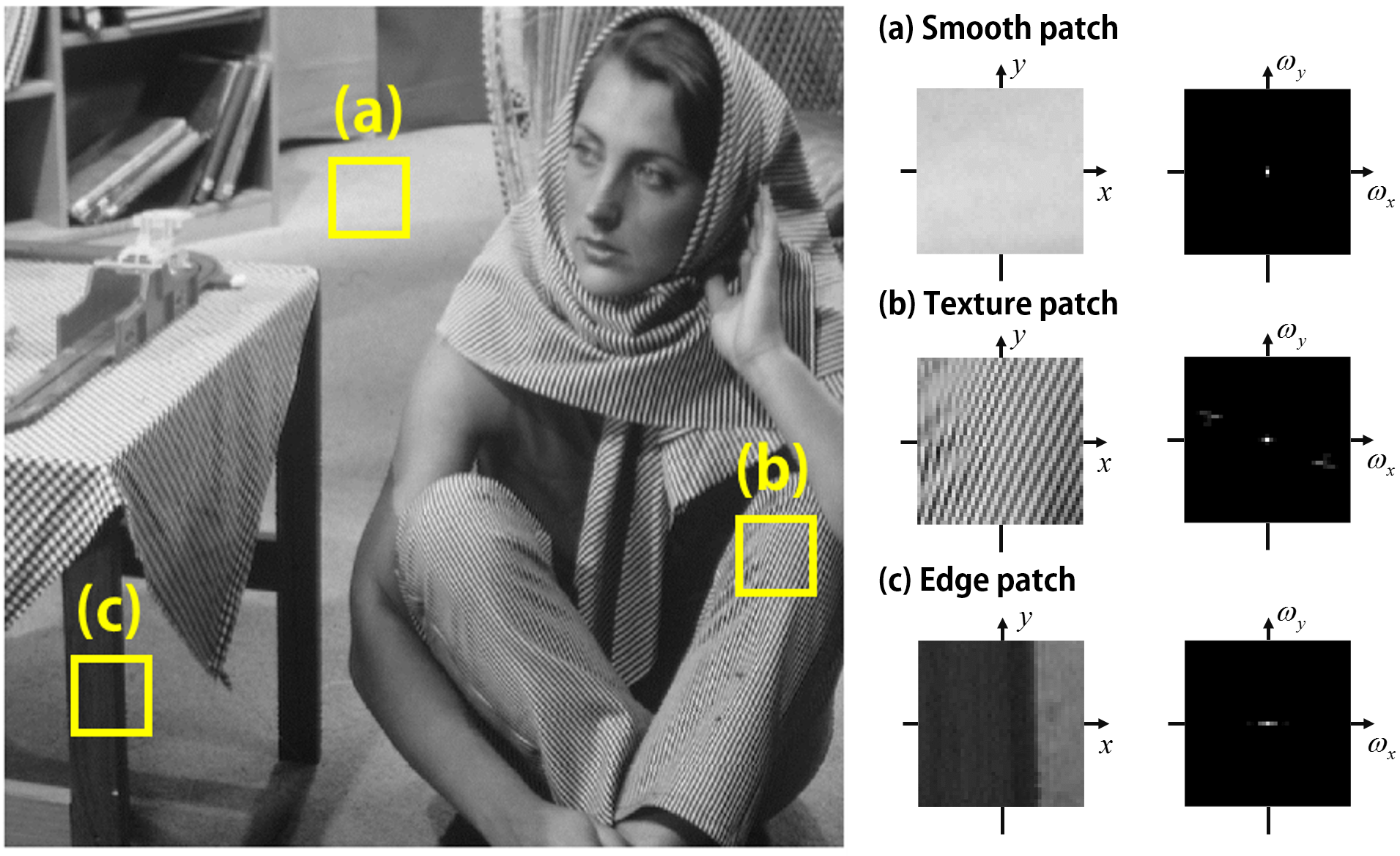
In our recent work [17], we demonstrate that diffusion [34, 35, 36, 37] and/or Gaussian Markov random field (GMRF) approaches for image modelling [38, 39, 40, 41, 42] are closely related to an annihilating filter relationship from the sampling theory of signals with finite rate of innovations (FRI) [18, 19]. More specifically, as shown in Fig. 1(a), a smoothly varying patch usually has spectrum content in the low frequency regions, and the other frequency regions have very little spectral components. A similar spectral domain sparsity can be observed in a texture patch in Fig. 1(b), where the spectral components are mainly concentrated on the fundamental frequencies of the patterns. For the case of an abrupt transition along the edge as shown in Fig. 1(c), the spectral components are mostly localized along the $\omega_{x}$ axis.

Mathematically, when a patch $x({\mathbf{r}})\in{\mathbb{R}}^{2}$ has sparse spectral components, we can show that there exists a corresponding annihilating filter in the image domain. More specifically, if the spectrum of an image patch is described by

$$\hat{x}(\bm{\omega})=\sum^{k-1}_{j=0}c_{j}\delta(\bm{\omega}-\bm{\omega}_{j}),~{}~{}\bm{\omega}=(\omega_{x},\omega_{y})$$ (2)

where $k$ denotes the number of non-zero spectral components, then it is easy to find an annihilating function $\hat{h}({\bm{\omega}})$ in the spectrum domain that does not overlap with the support of $\hat{x}({\bm{\omega}})$, i.e.

$$\hat{h}({\bm{\omega}})\hat{x}({\bm{\omega}})=0\,\quad\forall{\bm{\omega}}.$$ (3)

This implies the existence of the annihilating filter $h({\mathbf{r}}):=\mathcal{F}^{-1}\{\hat{h}({\bm{\omega}})\}$ in the image domain:

$$h({\mathbf{r}})\ast x({\mathbf{r}})=0.$$ (4)

For example, if an image is sufficiently flat with little variations in pixel values, then its spectral component $\hat{f}({\bm{\omega}})$ is most concentrated around the zero frequency component (i.e. $\hat{x}({\bm{\omega}})\simeq 0,{\bm{\omega}}\neq 0$); therefore, $\hat{h}({\bm{\omega}})=-\|{\bm{\omega}}\|^{2}$ becomes an annihilating function in the spectral domain. The associated annihilating filtering in the image domain is then given by

$$h({\mathbf{r}})\ast x({\mathbf{r}})=\Delta x({\mathbf{r}}).$$ (5)

where $\Delta$ denotes the Laplacian operator, which corresponds to the diffusion operation that is widely used in image denoising, inpainting, and so on [34, 35, 36, 37, 9, 10, 11]. This example clearly shows why the diffusion based approach is closely related to the annihilating filter approach.

If Fourier measurement data $\hat{x}({\bm{\omega}})$ is discretized at an appropriate Nyquist sampling rates, the corresponding discrete counterpart is given by

$$(h\ast x)[{\mathbf{n}}]=\sum_{{\mathbf{m}}}h[{\mathbf{m}}]x[{\mathbf{n}}-{\mathbf{m}}]=0,\quad{\mathbf{n}},{\mathbf{m}}\in\mathbb{Z}^{2},$$ (6)

where the discrete filter $h[{\mathbf{n}}]$ is now a discrete annihilating filter. Among the various of choices of annihilating function $\hat{h}({\bm{\omega}})$ that satisfies (3), Vetterli et al [18, 19] showed that an annihilating function can be constructed using a finite combination of sinusoidals such that the corresponding discrete annihilating filter $h[{\mathbf{n}}]$ has a finite filter length. In this case, the convolution (6) becomes finite length convolution, and we can exploit (6) in a matrix representation.

Specifically, let ${\mathbf{X}}\in{\mathbb{R}}^{N\times M}$ denote the matrix composed of $x[{\mathbf{n}}]$ such that ${\mathbf{X}}_{i,j}=x[i,j]$. We also define the discrete filter matrix ${\mathbf{H}}\in{\mathbb{R}}^{p\times q}$ such that ${\mathbf{H}}_{i,j}=h[i,j]$. Then, by removing the boundary data beyond the image patch, we can construct the following matrix equation:

$$\mathscr{H}\{{\mathbf{X}}\}\overline{\textsc{vec}({\mathbf{H}})}=\mathbf{0},$$ (7)

where ${\textsc{vec}({\mathbf{H}})}$ is the vectorisation of the matrix ${\mathbf{H}}$ and the overline is the order reversal operation. Moreover, the 2-D Hankel matrix $\mathscr{H}\{{\mathbf{X}}\}$ in (7) is defined by

$$\mathscr{H}\{{\mathbf{X}}\}= \!\left[\!\begin{array}[]{cccc}\!\mathfrak{h}\{{\mathbf{x}}_{1}\}&\mathfrak{h}\{{\mathbf{x}}_{2}\}&\cdots&\mathfrak{h}\{{\mathbf{x}}_{q}\}\\ \mathfrak{h}\{{\mathbf{x}}_{2}\}&\mathfrak{h}\{{\mathbf{x}}_{3}\}&\cdots&\mathfrak{h}\{{\mathbf{x}}_{q+1}\}\\ \vdots&\vdots&\ddots&\vdots\\ \mathfrak{h}\{{\mathbf{x}}_{N-q+1}\}&\mathfrak{h}\{{\mathbf{x}}_{N-2n+1}\}&\cdots&\mathfrak{h}\{{\mathbf{x}}_{N}\}\\ \end{array}\!\right]\!~{}\in{\mathbb{R}}^{(N-q+1)(M-p+1)\times pq}\ ,$$ (12)

and the 1-D Hankel matrix $\mathfrak{h}\{{\mathbf{x}}_{i}\}$ for the $i$-th column ${\mathbf{x}}_{i}$ of the matrix ${\mathbf{X}}$ is given by

$$\mathfrak{h}\{{\mathbf{x}}_{i}\}=\left[\begin{array}[]{cccc}x[1,i]&x[2,i]&\cdots&x[p,i]\\ x[2,i]&x[3,i]&\cdots&x[p+1,i]\\ \vdots&\vdots&\ddots&\vdots\\ x[M-p+1,i]&x[M-p+2,i]&\cdots&x[M,i]\end{array}\right]\ .$$

If the underlying signal has $k$-sparse spectral components, we can further show the following key result [20]:

$$\textsc{Rank}\mathscr{H}({\mathbf{X}})=k,\quad$$ (13)

which implies that as long as the annihilating filter size is bigger than the sparsity level, the rank of the associated Hankel matrix is always equal to the sparsity level. This implies the following duality:

$$\boxed{\mbox{$k$ spectral sparse image }~{}\overset{\mathcal{F}}{\longleftrightarrow}~{}\mbox{Rank-$k$ 2-D Hankel structure matrix}}$$

By exploiting this duality, our previous work [17] derived an annihilating filter-based low rank Hankel matrix approach for image inpainting. In this paper, this approach will be recasted into sparse+low rank decomposition for impulse noise removal.

II-C Sparse + Low-rank Decomposition Model for Hankel Structured Matrix from Impulse Noises

Figure 2: Sparse + low rank decomposition of Hankel structured matrix from an image patch corrupted with impulse noise. Because a lifting to Hankel structure is linear, the sparse impulse noises are also lifted to sparse outliers.

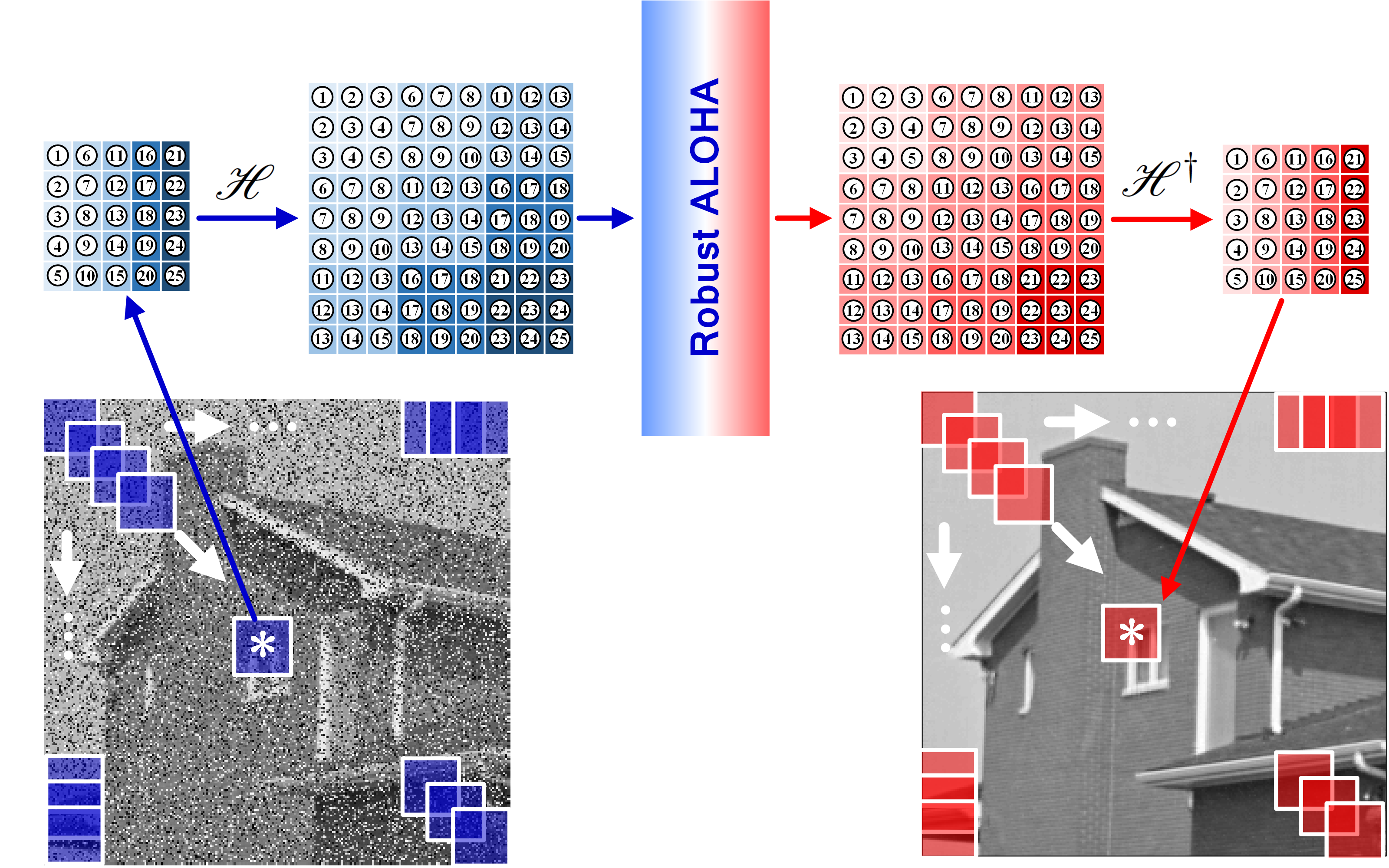
Unlike the lifting scheme used for phase retrieval problems [43], our lifting scheme to the Hankel structured matrix is linear, so the sparse impulse noise is also lifted to the sparse outliers in the lifted Hankel structured matrix (see Figure 2). Accordingly, if an underlying image is corrupted with sparse impulse noises, then we have

$$\mathscr{H}\{{\mathbf{X}}\}={\mathbf{L}}+{\mathbf{S}}$$ (14)

where ${\mathbf{L}}$ denotes the low-rank component and ${\mathbf{S}}$ represents the sparse components originated from impulse noises, which are both in the Hankel structure. This is the key property we want to exploit in our impulse noise removal algorithm. In fact, to address this type of sparse + low rank decomposition, the robust principal component analysis (RPCA) was actively investigated [26, 27, 28, 29, 30]. More specifically, for a given measurement matrix ${\mathbf{M}}$, the RPCA solves the following minimization problem:

$$\min \|{\mathbf{L}}\|_{\ast}+\tau\|{\mathbf{S}}\|_{1}$$ (15)

subject to $${\mathbf{L}}+{\mathbf{S}}={\mathbf{M}},$$ (16)

where $\|\cdot\|_{*}$ is the nuclear norm. To minimize this, alternating directions methods [44] were employed.

Compared to the standard RPCA approach, our sparse+ low rank decomposition problem using (14) requires additional constraint to impose Hankel structures. Therefore the RPCA algorithm should be modified. The specific optimization algorithm under this constraint will be explained in the following sections. Additionally, because the image statistics change across an image with spatially varying annihilating property, a noisy image should be partitioned into overlapped patches, which are processed patch-by-patch using robust ALOHA and the average values are used as described in the algorithm flowchart in Fig. 3.

Figure 3: Patch-by-patch processing framework using robust ALOHA for impulse noise removal.

III Optimization Methods

III-A Sparse + Low Rank Decomposition for Hankel Matrix

Note that the Hankel structure matrix in (12) is determined by the underlying image patch (${\mathbf{X}}$) size and the associated annihilating filter (${\mathbf{H}}$) size. For given $M\times N$ image patch and $p\times q$ annihilating filter, we now denote the associated spaces for the Hankel matrix as $\mathcal{H}(M,N;p,q)$. Then, for a given noisy image patch ${\mathbf{M}}\in{\mathbb{R}}^{M\times N}$ and $p\times q$ annihilating filter size, our impulse noise removal algorithm can be implemented by solving the following sparse + low rank decomposition under the Hankel structure matrix constraint:

$$(P)\quad \min_{{\mathbf{L}},{\mathbf{S}}} \|{\mathbf{L}}\|_{\ast}+\tau\|{\mathbf{S}}\|_{1}$$

subject to $${\mathbf{L}}+{\mathbf{S}}=\mathscr{H}\{{\mathbf{M}}\},$$

$${\mathbf{L}},{\mathbf{S}}\in\mathcal{H}(M,N;p,q)$$

Since the sparse components in image patch are also sparse in a lifted Hankel structure, ($P$) can be further simplified as

$$(P^{\prime})\quad \min_{{\mathbf{L}},{\mathbf{E}}} \|{\mathbf{L}}\|_{*}+\tau\|{\mathbf{E}}\|_{1}$$

subject to $${\mathbf{L}}=\mathscr{H}\{{\mathbf{X}}\}$$

$${\mathbf{X}}+{\mathbf{E}}={\mathbf{M}}.$$

where, with a slight abuse of notation, $\tau$ denotes an appropriately scaled version from $\tau$ in $(P)$. Note that ${\mathbf{E}}$ is now in image patch domain, unlike ${\mathbf{S}}$ in the lifted Hankel matrix structured matrix domain in $(P)$. The advantage of $(P^{\prime})$ over $(P)$ is an associated simpler optimization method. More specifically, if we apply a factorized form of nuclear norm relaxation [45], then the final problem formulation of the optimization problem can be expressed as

$$\min_{{\mathbf{E}},\{({\mathbf{U}},{\mathbf{V}})|{\mathbf{U}}{\mathbf{V}}^{H}=\mathscr{H}\{{\mathbf{X}}\}\}} \|{\mathbf{U}}\|_{F}^{2}+\|{\mathbf{V}}\|_{F}^{2}+\tau\|{\mathbf{E}}\|_{1}$$ (18)

subject to $${\mathbf{X}}+{\mathbf{E}}={\mathbf{M}}.$$ (19)

The constraints in (18) and (19) can be handled using alternating direction method of multiplier (ADMM) [32, 46, 28]. The associated Lagrangian function ADMM is given by:

$$L({\mathbf{U}},{\mathbf{V}},{\mathbf{E}},{\mathbf{X}},{\bm{\Theta}},{\bm{\Lambda}}):= \frac{1}{2}\left(\|{\mathbf{U}}\|_{F}^{2}+\|{\mathbf{V}}\|_{F}^{2}\right)+\tau\|{\mathbf{E}}\|_{1}+\frac{\beta}{2}\|{\mathbf{X}}+{\mathbf{E}}-{\mathbf{M}}+{\bm{\Theta}}\|_{F}^{2}+$$ (20)

$$\frac{\mu}{2}\|\mathscr{H}\{{\mathbf{X}}\}-{\mathbf{U}}{\mathbf{V}}^{H}+{\bm{\Lambda}}\|^{2}_{F}$$

Then, each subproblem is simply obtained from (20). More specifically, we have

$${\mathbf{E}}^{(k+1)} = \arg\min_{\mathbf{E}}\tau\|{\mathbf{E}}\|_{1}+\frac{\beta}{2}\|{\mathbf{X}}^{(k)}+{\mathbf{E}}-{\mathbf{M}}+{\bm{\Theta}}^{(k)}\|_{F}^{2}$$ (21)

$${\mathbf{X}}^{(k+1)} = \arg\min_{\mathbf{X}}\frac{\beta}{2}\|{\mathbf{X}}+{\mathbf{E}}^{(k+1)}-{\mathbf{M}}+{\bm{\Theta}}^{(k)}\|_{F}^{2}+\frac{\mu}{2}\|\mathscr{H}\{{\mathbf{X}}\}-{\mathbf{U}}^{(k)}{\mathbf{V}}^{(k)H}+{\bm{\Lambda}}^{(k)}\|^{2}_{F}$$ (22)

$${\mathbf{U}}^{(k+1)} = \arg\min_{\mathbf{U}}\frac{1}{2}\|{\mathbf{U}}\|_{F}^{2}+\frac{\mu}{2}\|\mathscr{H}\{{\mathbf{X}}^{(k+1)}\}-{\mathbf{U}}{\mathbf{V}}^{(k)H}+{\bm{\Lambda}}^{(k)}\|^{2}_{F}$$ (23)

$${\mathbf{V}}^{(k+1)} = \arg\min_{\mathbf{V}}\frac{1}{2}\|{\mathbf{V}}\|_{F}^{2}+\frac{\mu}{2}\|\mathscr{H}\{{\mathbf{X}}^{(k+1)}\}-{\mathbf{U}}^{(k+1)}{\mathbf{V}}^{H}+{\bm{\Lambda}}^{(k)}\|^{2}_{F}$$ (24)

$${\bm{\Theta}}^{(k+1)} = {\mathbf{X}}^{(k+1)}+{\mathbf{E}}^{(k+1)}-{\mathbf{M}}+{\bm{\Theta}}^{(k)}$$ (25)

$${\bm{\Lambda}}^{(k+1)} = \mathscr{H}\{{\mathbf{X}}^{(k+1)}\}-{\mathbf{U}}^{(k+1)}{\mathbf{V}}^{(k+1)H}+{\bm{\Lambda}}^{(k)}$$ (26)

It is easy to show that the first step can be simply reduced to a single soft-thresholding in image patch domain rather than in a lifted Hankel matrix space:

$${\mathbf{E}}^{(k+1)}=\mathcal{S}_{\tau/\beta}\left({\mathbf{M}}-{\mathbf{X}}^{(k)}-{\bm{\Theta}}^{(k)}\right)$$ (27)

where ${\mathcal{S}}_{\tau}$ denotes the pixel by pixel soft-thresholding with the threshold value $\tau$. The simple thresholding step in (27) is the main motivation which is why we prefer $(P^{\prime})$ over $(P)$. Now, the second step becomes

$${\mathbf{X}}^{(k+1)}=\frac{1}{\mu+\beta}\left(\mu\mathscr{H}^{{\dagger}}\left\{{\mathbf{U}}^{(k)}{\mathbf{V}}^{(k)H}-{\bm{\Lambda}}^{(k)}\right\}-\beta\left({\mathbf{E}}^{(k+1)}-{\mathbf{M}}+{\bm{\Theta}}^{(k)}\right)\right),$$ (28)

where $\mathscr{H}^{{\dagger}}$ corresponds to the Penrose-Moore pseduo-inverse mapping from our block Hankel structure to a patch, which is calculated as

$$\mathscr{H}^{{\dagger}}=\left(\mathscr{H}^{*}\mathscr{H}\right)^{-1}\mathscr{H}^{*}\ .$$ (29)

Note that the adjoint operator $\mathscr{H}^{*}\{{\mathbf{A}}\}$ adds multiple elements of ${\mathbf{A}}$ and put it back to the patch coordinate, and $\left(\mathscr{H}^{*}\mathscr{H}\right)^{-1}$ denotes the division by the number of multiple correspondence; hence, the role of the pseudo-inverse is taking the average value and put it back to the patch coordinate. Next, the subproblems for ${\mathbf{U}}$ and ${\mathbf{V}}$ can be easily calculated by taking the derivative with respect to each matrix. For example, the derivative of cost function for ${\mathbf{U}}$ is given by

$$\frac{\partial L}{\partial{\mathbf{U}}} = \frac{\partial}{\partial{\mathbf{U}}}\left(\frac{1}{2}\|{\mathbf{U}}\|_{F}^{2}+\frac{\mu}{2}\|\mathscr{H}\{{\mathbf{X}}\}-{\mathbf{U}}{\mathbf{V}}^{H}+{\bm{\Lambda}}\|^{2}_{F}\right)$$

$$= {\mathbf{U}}-\mu\left(\mathscr{H}\{{\mathbf{X}}\}-{\mathbf{U}}{\mathbf{V}}^{H}+{\bm{\Lambda}}\right){\mathbf{V}}$$

$$= {\mathbf{U}}\left(I+\mu{\mathbf{V}}^{H}{\mathbf{V}}\right)-\mu\left(\mathscr{H}\{{\mathbf{X}}\}+{\bm{\Lambda}}\right){\mathbf{V}},$$

and the closed-form solution of the subproblem for ${\mathbf{U}}$ is obtained by setting $\partial L/\partial{\mathbf{U}}=0$. In the similar way, the derivative with respect to ${\mathbf{V}}$ can be obtained. Accordingly, the closed-form update equations for ${\mathbf{U}}$ and ${\mathbf{V}}$ are given by

$${\mathbf{U}}^{(k+1)} = \mu\left(\mathscr{H}\{{\mathbf{X}}^{(k+1)}\}+{\bm{\Lambda}}^{(k)}\right){\mathbf{V}}^{(k)}\left(I+\mu{\mathbf{V}}^{(k)H}{\mathbf{V}}^{(k)}\right)^{-1}$$ (30)

$${\mathbf{V}}^{(k+1)} = \mu\left(\mathscr{H}\{{\mathbf{X}}^{(k+1)}\}+{\bm{\Lambda}}^{(k)}\right)^{H}{\mathbf{U}}^{(k+1)}\left(I+\mu{\mathbf{U}}^{(k+1)H}{\mathbf{U}}^{(k+1)}\right)^{-1}.$$ (31)

Even though the original Hankel matrix $\mathscr{H}\{{\mathbf{X}}\}$ has large dimension, it is important to note that our algorithm using (30) and (31) only require the matrix inversion of $k\times k$ matrix, where $k$ denotes the estimated rank of the Hankel matrix. This significantly reduces the overall computational complexity.

Before we apply ADMM, the initial estimatel ${\mathbf{U}}$ and ${\mathbf{V}}$ have to be determined with an estimated rank. For this, we employed an SVD-free algorithm called low-rank factorization model (LMaFit) [33]. More specifically, for a low-rank matrix ${\mathbf{Z}}$, LMaFit solves the following optimization problem:

$$\min_{{\mathbf{U}},{\mathbf{V}},{\mathbf{Z}}}~{}\frac{1}{2}\|{\mathbf{U}}{\mathbf{V}}^{H}-{\mathbf{Z}}\|^{2}_{F}~{}$$ (32)

and ${\mathbf{Z}}$ is initialized with $\mathscr{H}\{{\mathbf{M}}\}$. LMaFit solves a linear equation with respect to ${\mathbf{U}}$ and ${\mathbf{V}}$ to find their updates and relaxes the updates by taking the average between the previous iterations. Moreover, the rank update can be done automatically by detecting the abrupt changes of diagonal elements of QR factorization [33]. Even though the problem (32) is non-convex due to the multiplication of ${\mathbf{U}}$ and ${\mathbf{V}}$, the convergence of LMaFit to a stationary point was analyzed in detail [33]. However, the LMaFit alone cannot recover the block Hankel structure, which is the reason we use ADMM later to impose the structure.

IV Extension to Multi-channel Impulse Noise Removal

In many applications, images are obtained through multiple measurement channels. For example, in a colour image, multiple images are measured throughout R (red), G (green) and B (blue) detectors. In multispectral imaging for remote sensing applications, a scene is measured through many spectral bands. In these applications, the underlying structure is identical so that there exists strong correlation between different channel measurements. Regarding the random impulse noise contamination, we may encounter two different scenarios: 1) noisy pixel locations are independent between the channels, and 2) noisy pixel locations are same across the channels. The first scenario is commonly observed when independent detectors are used for each channel. On the other hand, when a spectrometer is used to split an input into multiple channels, then the noisy pixel locations should be common across the channel. Therefore, in this section, we are interested in extending single-channel robust ALOHA to address these two cases.

IV-A Multi-Channel Image Modeling

Figure 4: (a) Spectral distribution across channels. (b) Multi-channel measurement model.

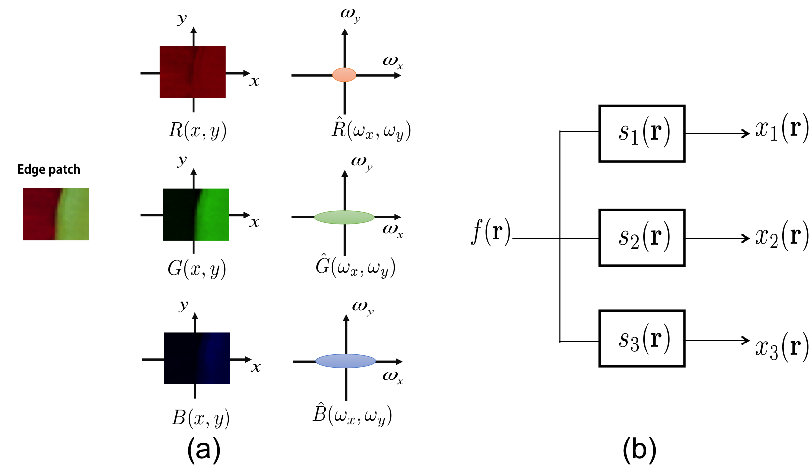
Let $f({\mathbf{r}})$ denote an underlying image patch that are common for all channel measurements, and $\hat{f}({\bm{\omega}})$ be its spectrum. Then, as shown in Fig. 4(a), the spectrum of the $i$-th channel measurement can be modeled as:

$$\hat{x}_{i}({\bm{\omega}})=\hat{s}_{i}({\bm{\omega}})\hat{f}({\bm{\omega}}),\quad i=1,\cdots,C,$$ (33)

where $\hat{s}_{i}({\bm{\omega}})$ denotes a spectral modulation function of the $i$-th channel. The model (33) assumes that each channel measurements still retains the textures of the underlying images with a channel specific modulation, which property was previously extensively used in multichannel deconvolution problems [47, 48, 49] illustrated in Fig. 4(b). As a result, it is easy to derive the following inter-channel annihilating filter relation:

$$s_{j}({\mathbf{r}})\ast x_{i}({\mathbf{r}})-s_{i}({\mathbf{r}})\ast x_{j}({\mathbf{r}})=0,\quad\forall{\mathbf{r}},~{}~{}i\neq j,$$ (34)

which was also a key property in these multichannel devolution algorithms [47, 48, 49].

To exploit the inter-channel annihilating property in our robust ALOHA, we construct the following matrix:

$${\bm{\mathcal{Y}}}=\left[\mathscr{H}\{{\mathbf{X}}_{1}\}~{}\mathscr{H}\{{\mathbf{X}}_{2}\}~{}\cdots~{}\mathscr{H}\{{\mathbf{X}}_{C}\}\right]~{}\in{\mathbb{R}}^{(N-q+1)(M-p+1)\times Cpq}$$ (35)

where $\mathscr{H}\{{\mathbf{X}}_{i}\}$ denotes the Hankel structured matrix constructed from the $i$-th channel measurement $x_{i}({\mathbf{r}})$. Then, it is easy to show that

$${\bm{\mathcal{Y}}}\mathcal{S}_{1}=\mathbf{0},$$

where $\mathcal{S}_{1}$ is defined recursively as follows:

$$\mathcal{S}_{C-1} \triangleq \left[\begin{array}[]{cc}\bar{\mathbf{s}}_{C}\\ -\bar{\mathbf{s}}_{C-1}\\ \end{array}\right]$$ (38)

$$\mathcal{S}_{t} \triangleq \left[\begin{array}[]{cccc|c}\bar{\mathbf{s}}_{t+1}&\bar{\mathbf{s}}_{t+2}&\cdots&\bar{\mathbf{s}}_{C}&\mathbf{0}\\ \hline\cr-\bar{\mathbf{s}}_{t}&&&&\\ &-\bar{\mathbf{s}}_{t}&&&\mathcal{S}_{t+1}\\ &&\ddots&\\ &&&-\bar{\mathbf{s}}_{t}&\end{array}\right]\ ,$$ (44)

and $\bar{\mathbf{s}}_{i}:=\overline{\textsc{vec}({\mathbf{S}}_{i})}$ denotes the reversed ordered, vectored spectral modulation filter for the $i$-th channel. Because $\dim\textsc{Nul}({\bm{\mathcal{Y}}})=\mathrm{rank}(\mathcal{S}_{1})=\binom{C}{2}={C(C-1)}/{2},$ we have

$$\mathrm{rank}~{}{\bm{\mathcal{Y}}} \leq kC-\frac{C(C-1)}{2}=\frac{C(2k-C+1)}{2}\ ,$$ (45)

when the underlying spectrum $\hat{f}({\bm{\omega}})$ is $k$-sparse. Hence, by choosing the annihilating filter size sufficiently large, we can make ${\bm{\mathcal{Y}}}$ low-ranked and the aforementioned sparse+ low rank model can be used for impulse noise removal.

IV-B Optimization Methods

IV-B1 Channel independent impulse noises

When the locations of the impulse noise are independent between channels, then the associate optimization problem is very similar to that of the single channel problem. More specifically, if we define

$${\mathbf{M}}=\begin{bmatrix}{\mathbf{M}}_{1}|\cdots|{\mathbf{M}}_{C}\end{bmatrix},\quad{\mathbf{X}}=\begin{bmatrix}{\mathbf{X}}_{1}|\cdots|{\mathbf{X}}_{C}\end{bmatrix},\quad{\mathbf{E}}=\begin{bmatrix}{\mathbf{E}}_{1}|\cdots|{\mathbf{E}}_{C}\end{bmatrix}$$ (46)

such that the each channel measurement is give by

$${\mathbf{M}}_{i}={\mathbf{X}}_{i}+{\mathbf{E}}_{i},$$

then the optimization problem becomes

$$\min_{{\mathbf{E}},\{({\mathbf{U}},{\mathbf{V}})|{\mathbf{U}}{\mathbf{V}}^{H}={\bm{\mathcal{Y}}}\}} \|{\mathbf{U}}\|_{F}^{2}+\|{\mathbf{V}}\|_{F}^{2}+\tau\|{\mathbf{E}}\|_{1}$$ (47)

subject to $${\bm{\mathcal{Y}}}=\left[\mathscr{H}\{{\mathbf{X}}_{1}\}~{}\mathscr{H}\{{\mathbf{X}}_{2}\}~{}\cdots~{}\mathscr{H}\{{\mathbf{X}}_{C}\}\right]$$ (48)

$${\mathbf{X}}+{\mathbf{E}}={\mathbf{M}}\ .$$

In this case, the Lagrangian cost function and the associated subproblems are same as Eq. (20) and (22)-(28), respectively.

IV-B2 Common impulse noise locations

When the noisy pixel locations are common across the channels, we need a major algorithmic change that comes from a common sparsity inducing matrix norm penalty. More specifically, a common support condition of sparse components ${\mathbf{E}}$ should be imposed across channels. In this paper, this constraint is formulated using the group-wise mixed $l_{1,2}$ norm:

$${\mathbf{E}}=\begin{bmatrix}{\mathbf{E}}_{1}|\cdots|{\mathbf{E}}_{C}\end{bmatrix}\quad\Longrightarrow\quad\|{\mathbf{E}}\|_{1,2}:=\sum_{i,j}\sqrt{\sum_{k=1}^{C}{\mathbf{E}}_{k}(i,j)^{2}}$$ (49)

Then, Eq. (20) can be converted to

$$L({\mathbf{U}},{\mathbf{V}},{\mathbf{E}},{\mathbf{X}},{\bm{\Theta}},{\bm{\Lambda}}):= \frac{1}{2}\left(\|{\mathbf{U}}\|_{F}^{2}+\|{\mathbf{V}}\|_{F}^{2}\right)+\tau\|{\mathbf{E}}\|_{1,2}+\frac{\beta}{2}\|{\mathbf{X}}+{\mathbf{E}}-{\mathbf{M}}+{\bm{\Theta}}\|_{F}^{2}+$$ (50)

$$\frac{\mu}{2}\|\mathscr{H}\{{\mathbf{X}}\}-{\mathbf{U}}{\mathbf{V}}^{H}+{\bm{\Lambda}}\|^{2}_{F}.$$

Then, instead of using (21), the corresponding subproblem for ${\mathbf{E}}$ has the following closed form solution [50]:

$${\mathbf{E}}^{(k+1)} = \mathcal{S}^{{ch}}_{\tau/\beta}\left({\mathbf{M}}-{\mathbf{X}}^{(k)}-{\bm{\Theta}}^{(k)}\right)$$ (51)

where, for ${\mathbf{E}}$ in (49), $\mathcal{S}^{{ch}}_{\lambda}({\mathbf{E}})$ is defined as

$$\mathcal{S}^{{ch}}_{\lambda}\left({\mathbf{E}}\right):=\begin{bmatrix}\mathcal{S}^{{vec}}_{\lambda}({\mathbf{E}}_{1})|\cdots|\mathcal{S}^{{vec}}_{\lambda}({\mathbf{E}}_{C})\end{bmatrix}$$

and

$$\left[\mathcal{S}^{{vec}}_{\lambda}({\mathbf{E}}_{k})\right]_{ij}=\frac{{\mathbf{E}}_{k}(i,j)}{\sqrt{\sum_{k=1}^{C}|{\mathbf{E}}_{k}(i,j)|^{2}}}\max\left\{\sqrt{\sum_{k=1}^{C}|{\mathbf{E}}_{k}(i,j)|^{2}}-\lambda,0\right\}\ .$$ (52)

Other remaining subproblems are same with (22)-(28).

V Experimental Results

V-A Removal of Random Valued Impulse Noise (RVIN)

We first performed denoising experiments using randomly distributed random valued impulse noise (RVIN) that corrupts 25% and 40% of the whole image pixels. The RVIN is given as follows. Let $x_{ij}:={\mathbf{X}}(i,j)$ and $N(x_{ij})$ be the original pixel value at location $(i,j)$ and the contaminated pixel with impulse noise at location $(i,j)$, respectively. When the dynamic range of pixel value is given as $\left[d_{{min}}~{}d_{{max}}\right]$, RVIN is described as

$$N(x_{ij})=\begin{cases}d_{ij}&\quad\text{ with probability $p$}\\ x_{ij}&\quad\text{ with probability $1-p$}\end{cases}$$ (53)

where $d_{ij}$ is a random number between $\left[d_{{min}}~{}d_{{max}}\right]$ chosen by the uniform random probability density function and $p$ is the proportion of noisy pixels with respect to total pixels.

The test sets were Baboon, Barbara, Boat, Cameraman, House, Lena and Peppers images. All test images were rescaled to have values between 0 and 1. For comparison, a median filter method (MATLAB built-in function ‘medfilt2’, indicated as MF in the figures) was used as the simplest reference algorithm, and the existing algorithms such as ACWMF[3], and TVL1[51] were also used. The original codes from the original authors were used and the parameters for the comparative algorithms were optimized to have the best performances. The parameters for the proposed method are given in Table. I. The maximum iteration number of ADMM in Eq. (20) was set to $500$, and the stopping criteria was defined as in [33] with the tolerance set to $10^{-4}$. For quantitative evaluation, we used the PSNR (peak signal-to-noise ratio). Specifically, when the reference signal (${\mathbf{y}}$) is given, the PSNR of the reconstructed image (${\mathbf{x}}$) is calculated as

$$\mbox{PSNR}({\mathbf{x}})=20\log_{10}\left(\frac{\|{\mathbf{y}}\|_{\infty}}{1/\sqrt{N}\times\|{\mathbf{y}}-{\mathbf{x}}\|_{2}}\right).$$

TABLE I: Hyper-parameters used in the proposed algorithm. $\mu$ and $\beta$ of ADMM are $1$. For LMaFit, initial rank with increasing strategy is one and tolerances for $25\%(40\%)$ impulse noise is $0.2(0.3)$.

	Baboon	Barbara	Boat	Cameraman	House	Lena	Peppers
	($512\times 512$)	($512\times 512$)	($512\times 512$)	($256\times 256$)	($256\times 256$)	($512\times 512$)	($255\times 255$)
Size of ${\mathbf{X}}$	$45\times 45$	$25\times 25$	$25\times 25$	$31\times 31$	$25\times 25$	$25\times 25$	$25\times 25$ ($45\times 45$)
Size of ${\mathbf{H}}$	$13\times 13$	$11\times 11$	$11\times 11$	$13\times 13$	$11\times 11$	$11\times 11$	$9\times 9$ ($13\times 13$)
Size of $\mathscr{H}\{{\mathbf{X}}\}$	$1089\times 169$	$225\times 121$	$225\times 121$	$361\times 169$	$225\times 121$	$225\times 121$	$289\times 81(1089\times 169)$
$\tau(\times 10^{-2})$	$10~{}(7.5)$	$10$	$10$	$10~{}(7.5)$	$10$	$10$	$10~{}(7.5)$

TABLE II: Reconstruction image PSNR by various denoising algorithms from 25% and 40% random valued impulse noise (RVIN). The highest PSNR in each image are highlighted with boldface.

		Noisy image	MF	ACWMF	TVL1	Proposed
Baboon	25%	15.53	22.01	23.14	23.39	24.82
	40%	13.52	20.52	21	21.68	22.46
Barbara	25%	14.84	23.62	24.59	24.99	33.13
	40%	12.82	21.14	22.86	23.43	28.51
Boat	25%	15.37	27.27	28.09	28.64	30.57
	40%	13.31	23.52	25.73	26.19	26.89
Cameraman	25%	14.44	24.28	24.69	25.58	26.74
	40%	12.37	20.61	22.13	23	23.44
House	25%	15.31	29.08	29.74	31.16	34.29
	40%	13.27	24.36	27.44	28.07	28.99
Lena	25%	15.29	30.07	30.75	31.9	34.31
	40%	13.23	24.6	28.78	29.14	30.48
Peppers	25%	14.99	27.47	27.91	29.09	29.47
	40%	12.96	23.15	25.66	26.07	26.26

Figure 5: Reconstructed Barbara images by various methods from 40% random valued impulse noise.

Figure 6: ${\mathbf{M}}$: the measured noisy image. $|\mbox{ORIG}-{\mathbf{M}}|$: the residual image between noisy image and original image. ${\mathbf{X}}$: the decomposed low-rank part, and ${\mathbf{E}}$: the decomposed sparse component.

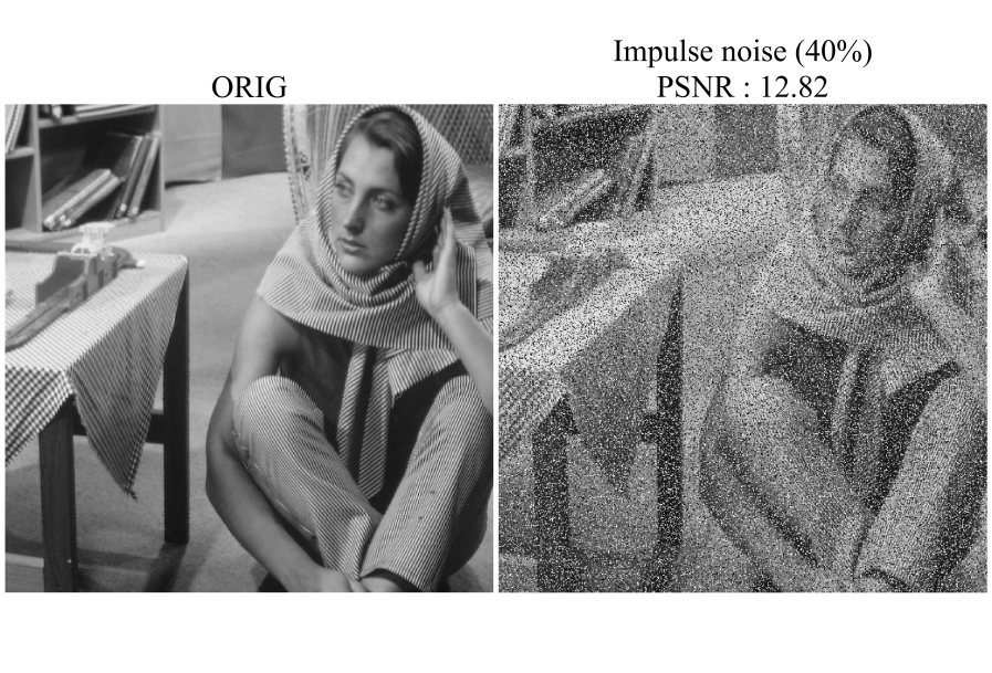
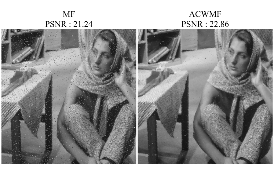
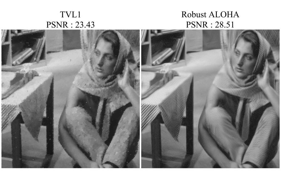
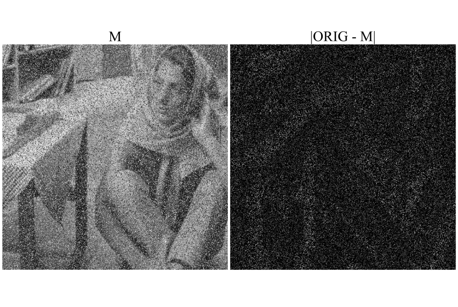
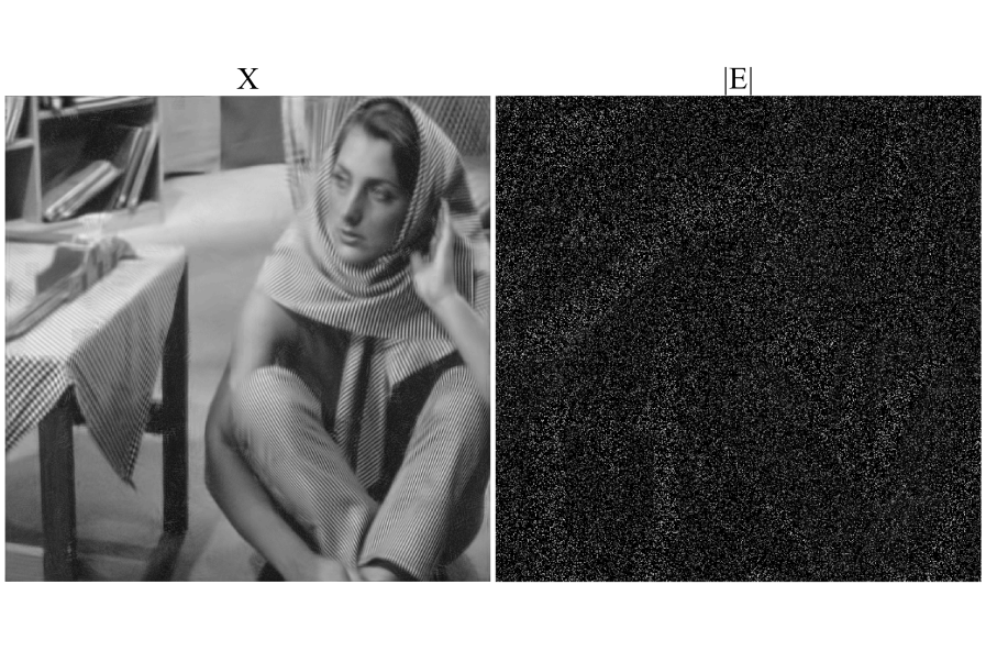
We summarized the PSNR results in Table II for all reconstructed images. The proposed method outperformed all other algorithms in both PSNR and visual quality, and the PSNR improvement was up to 8dB. Fig. 5 is the typical reconstruction result that shows noticeable enhancement in both visual quality and quantitative measures. In order to show that the proposed sparse+ low rank decomposition properly decomposes the impulse noises from the images, the decomposed sparse and low-rank components are illustrated in Fig. 6. We can see that sparse component ($|{\mathbf{E}}|$) looks similar to the additive impulse noises as indicated by $|\mbox{ORIG}-{\mathbf{M}}|$.

V-B Salt and Pepper Noise

The salt and pepper noise is a special case of RVIN, because it has impulse noises with the intensity of the minimum and maximum values of pixel dynamic range. Specifically, the salt and pepper noises are given by

$$N(x_{ij})=\begin{cases}d_{min}&\quad\text{ with probability $p/2$}\\ d_{max}&\quad\text{ with probability $p/2$}\\ x_{ij}&\quad\text{ with probability $1-p$}\\ \end{cases}$$ (54)

where variables $p,~{}d_{max},~{}d_{min}$ were defined in Eq. (53).

Figure 7: Salt and pepper noise removal results using various methods.

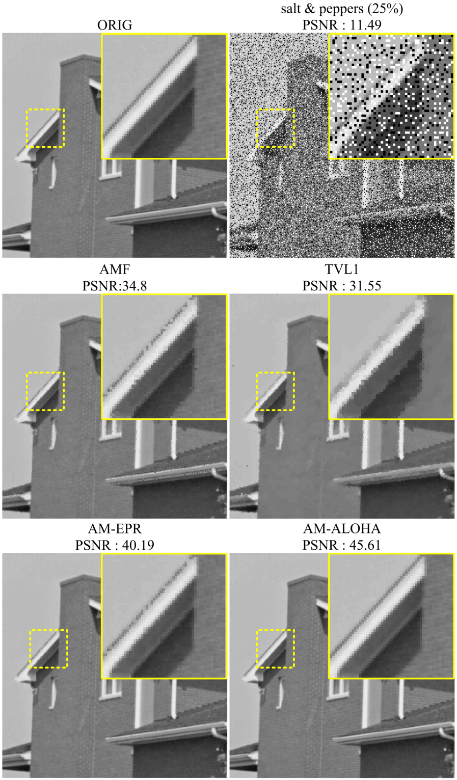
Due to the extremal pixel values, the salt and pepper noise can be exceptionally well detected by adaptive median filter (AMF), so the AMF-based denoising algorithms with edge preserving prior (AM-EPR) have been proposed [1]. If the position of the salt and noise locations are well detected by AMF, our robust ALOHA can be modified accordingly. More specifically, the estimation of the sparse component ${\mathbf{E}}$ in (18) and (19) is no more necessary, and the resulting algorithm becomes identical to the ALOHA image inpainting algorithm [17]. We denote this modification using AMF as AM-ALOHA. To demonstrate that our algorithm still outperforms the existing algorithms, we compared our method with median filtering (MF), adaptive median filtering (AMF), AMF-based denoising algorithms with edge preserving prior (AM-EPR) using 25 % salt and pepper noise. The results in Fig. 7 clearly demonstrates that the proposed AM-ALOHA outperforms all other algorithms.

V-C Multi-channel Denoising

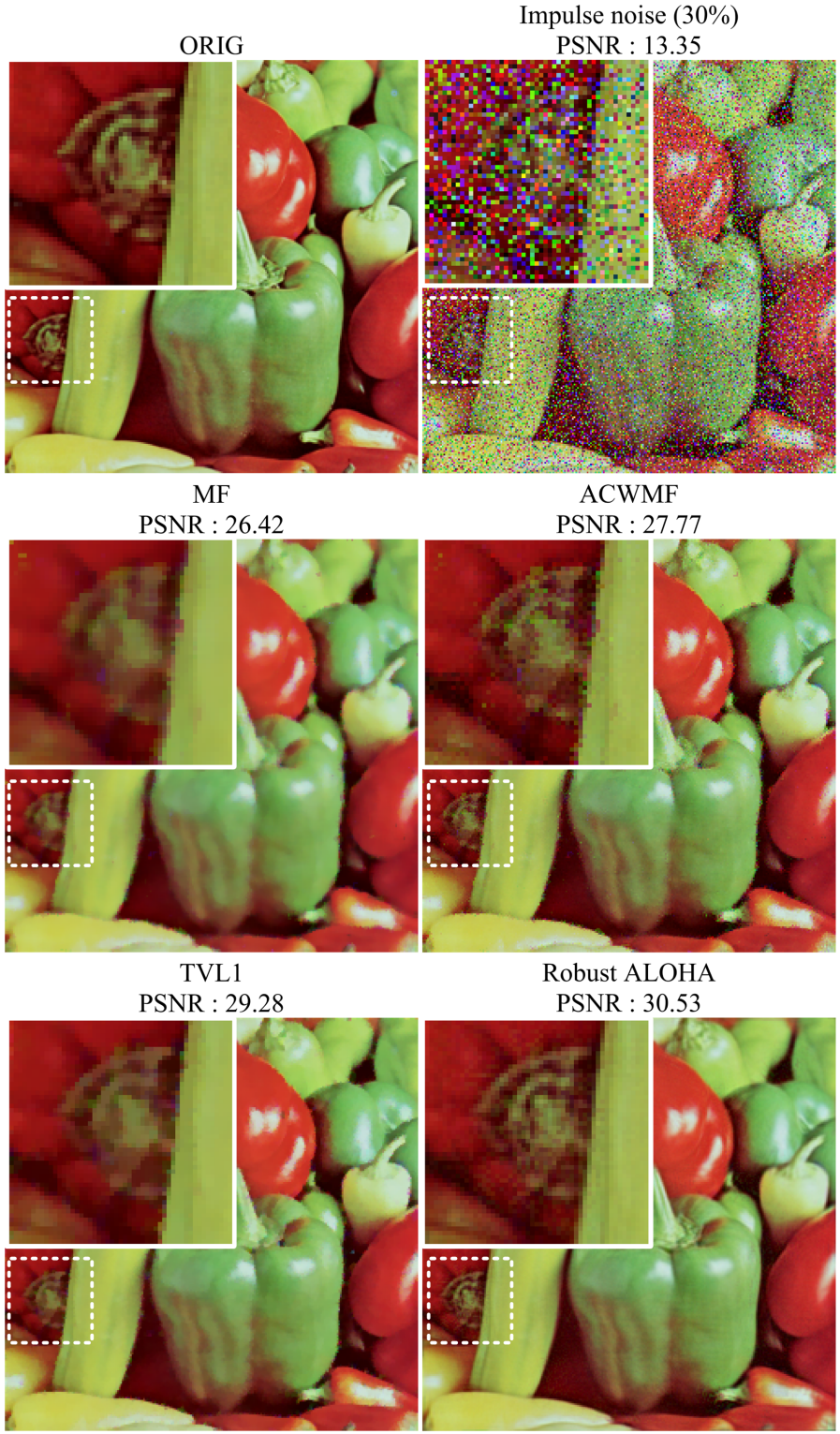
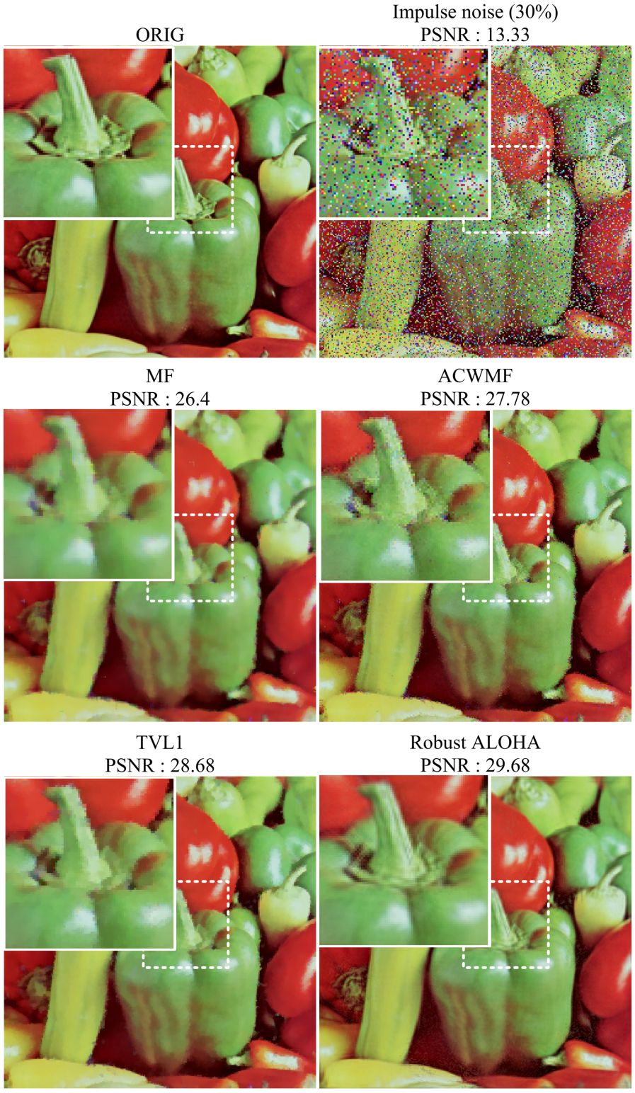
To verify that the proposed method can be easily extended to multichannel images, we conducted experiments with colour RGB images. As discussed before, the noisy pixel location can be either same across channels or independent for each channel. So we conducted experiments under the two different scenarios. Fig. 8 showed the reconstruction result when $30\%$ channel independent impulse noises were added, whereas Fig. 9 corresponds to the scenario when $30\%$ of impulse noises were added at the same locations across RGB channels. The proposed method provided better detailed structures (e.g. bundle of peppers and the edges of peppers) than TVL1 method as shown in Figs. 8-9. Also, the cartoon-like artifacts were significantly reduced in the proposed method. In the inset images, the detail structures of peppers are magnified to demonstrate superior performance of the proposed method over TVL1.

One of the interesting observations from these experiments was that the proposed reconstruction provided a better PSNR for the channel independent impulse noises. This was because the noiseless pixel values from other channels could improve the image inpainting performance of noisy pixel values by exploiting the correlation between the channels.

Figure 8: Multi-channel denoising results under 30% random valued impulse noises at the independent pixel locations at each RGB channels.

Figure 9: Multi-channel denoising results under 30% random valued impulse noises at the common pixel locations across the RGB channels.

V-D Comparison with conventional RPCA

Figure 10: Comparison with conventional RPCA approach with the proposed method under 40% random valued impulse noises.

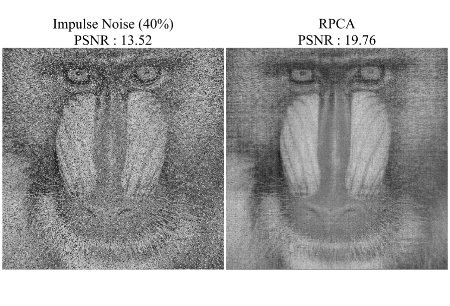
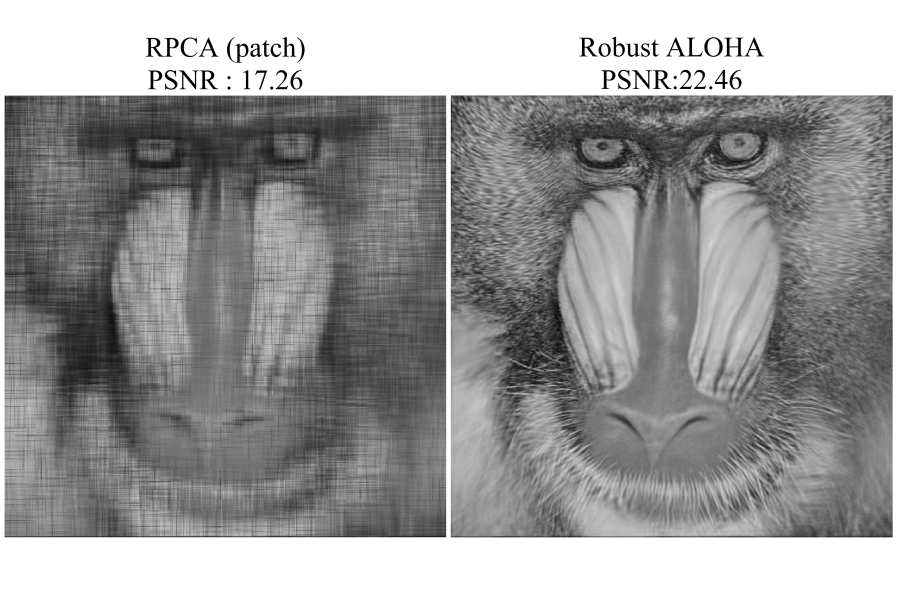
To verify that a lifting to a Hankel matrix is essential for performance improvement, we applied the standard RPCA as an impulse noise removal algorithm and compared the results. Two types of RPCA were implemented: one using whole images, and the other using image patch of the same size as our robust ALOHA. Note that the standard RPCA uses an image or patches as they are, without reformulating them into a Hankel structured matrix. For RPCA, we used the software packages provided by the original authors in [29]. We chose the parameters for the best PSNR results in each reconstruction. As you can see in Fig. 10, two forms of RPCA implementations completely failed in removing impulse noises, and the detailed image structures were distorted. On the other hand, the robust ALOHA provided nearly perfect noise removal. Such a remarkable performance improvement was originated from an image modeling using a low rankness of annihilating filter-based Hankel matrix, which again confirm the robust ALOHA is a superior image model and denoising algorithm for images corrupted with impulse noises.

VI Discussion

Recall that the proposed robust ALOHA was performed patch by patch without considering additional similar patches. This is of great importance in contrast to other denoising algorithms that use low-rank approaches [16, 52, 53, 54]. While the authors in [16, 52, 53, 54] used the patch-based low-rankness, all methods required additional redundancies from, for example, multiple dynamic frames [16, 52] or groups of similar spectral patches [53, 54]. Even though such additional redundant information may introduce a low-rankness, those approaches could not properly perform denoising without utilising such additional redundancies. On the other hand, the robust ALOHA exploits the low-rankness originated from intrinsic spectral sparsity of an image patch, so no additional redundancy is necessary. Thus, it is more flexible and powerful.

As briefly discussed in the introduction, a recent research [31] successfully demonstrated accurate prediction of target locations under occlusion using sparse $+$ low rank decomposition of Hankel structured matrix. However, unlike our robust ALOHA, one-dimensional trajectories extracted from video sequences are required as inputs to construct the Hankel structured matrix, because the algorithm was derived based on the assumption that those trajectories follow the linear time invariant state-space models, which was first suggested in [55]. On the other hand, the Hankel structured matrix in robust ALOHA is derived from two dimensional patches by exploiting the spectral domain sparsity; thus, the construction of the Hankel matrix is different from [31]. Moreover, we exploit an SVD-free minimization algorithm [46] instead of an augmented Lagrangian method (ALM) in [31, 55] for saving computational burdens. Therefore, we believe that there exist significant differences between the two approaches.

From the sampling theory point of view, a recent paper by Chen and Chi [56] provides a theoretical estimate of fundamental performance of our robust ALOHA. In [56], the authors showed that the required number of samples, $m$, for the recovery of signal $\mathscr{H}\{{\mathbf{X}}\}$ with ${\mathbf{X}}\in{\mathbb{R}}^{M\times N}$ corrupted with sparse outlier ${\mathbf{E}}$ using (P) in (III-A) is given by

$$m>c_{1}\mu_{1}^{2}c_{s}^{2}r^{2}\log^{3}(MN),$$ (55)

when the regularization parameter in (III-A) is given by $\tau=1/\sqrt{m\log(MN)}$ and the a noise corruption fraction is smaller than $20\%$. In (55), $c_{1}>0$ is a numerical constant depending on the corruption fraction, $\mu_{1}$ is incoherence parameter, $c_{s}:=\max\left\{\frac{MN}{pq},\frac{MN}{(M-p+1)(N-q+1)}\right\}$ , and $r$ is the rank of single channel Hankel matrix. Because $m=MN$ in our robust ALOHA for impulse noise removal, the theoretical result in (55) strongly supports our finding that as long as the spectrum of a patch is sufficiently sparse, the proposed sparse and low-rank method can restore the corrupted signal even with significant impulse noises (in our simulation, up to 40 $\%$).

VII Conclusion

In this paper, we proposed a sparse + low rank decomposition of annihilating filter-based Hankel matrices for impulse noise removal. The new algorithm, called robust ALOHA, extends the conventional RPCA approaches by exploiting the spectral domain sparsity and the associated rank deficient Hankel matrix. The robust ALOHA was implemented using ADMM iteration with initialization using LMaFit algorithms. In our ADMM formulation, factorization based nuclear norm minimization, was used instead of SVD so that the computational gain is achieved. We demonstrated that the robust ALOHA outperformed the existing impulse noise removal algorithms up to 8dB. Furthermore, we showed that the robust ALOHA can be used for salt and pepper noises by incorporating the estimated noise locations. In addition, the extension to impulse noise removals from colour channels was very straightforward by concatenating the Hankel structure matrix side by side and imposing the low-rankness.

The superior performance of the robust ALOHA as well as ALOHA inpainting [17] clearly shows that image modeling using annihilating filter based Hankel matrix is a very powerful tool with many image processing applications.

References

- [1] R. H. Chan, C.-W. Ho, and M. Nikolova, “Salt-and-pepper noise removal by median-type noise detectors and detail-preserving regularization,” Image Processing, IEEE Transactions on, vol. 14, no. 10, pp. 1479–1485, 2005.
- [2] H. Hwang, R. Haddad et al., “Adaptive median filters: new algorithms and results,” IEEE Trans. Image Process., vol. 4, no. 4, pp. 499–502, 1995.
- [3] T. Chen and H. R. Wu, “Adaptive impulse detection using center-weighted median filters,” IEEE Signal Process. Lett., vol. 8, no. 1, pp. 1–3, 2001.
- [4] M. Yan, “Restoration of images corrupted by impulse noise and mixed gaussian impulse noise using blind inpainting,” SIAM Journal on Imaging Sciences, vol. 6, no. 3, pp. 1227–1245, 2013.
- [5] T. Chen and H. R. Wu, “Space variant median filters for the restoration of impulse noise corrupted images,” IEEE Transactions on Circuits and Systems II: Analog and Digital Signal Processing, vol. 48, no. 8, pp. 784–789, 2001.
- [6] H.-L. Eng and K.-K. Ma, “Noise adaptive soft-switching median filter,” IEEE Trans. Image Process., vol. 10, no. 2, pp. 242–251, 2001.
- [7] G. Pok, J.-C. Liu, and A. S. Nair, “Selective removal of impulse noise based on homogeneity level information,” IEEE Trans. Image Process., vol. 12, no. 1, pp. 85–92, 2003.
- [8] M. Nikolova, “A variational approach to remove outliers and impulse noise,” Journal of Mathematical Imaging and Vision, vol. 20, no. 1-2, pp. 99–120, 2004.
- [9] A. Chambolle and T. Pock, “A first-order primal-dual algorithm for convex problems with applications to imaging,” Journal of Mathematical Imaging and Vision, vol. 40, no. 1, pp. 120–145, 2011.
- [10] J. Yang, Y. Zhang, and W. Yin, “An efficient TVL1 algorithm for deblurring multichannel images corrupted by impulsive noise,” SIAM Journal on Scientific Computing, vol. 31, no. 4, pp. 2842–2865, 2009.
- [11] S. H. Chan, R. Khoshabeh, K. B. Gibson, P. E. Gill, and T. Q. Nguyen, “An augmented Lagrangian method for total variation video restoration,” IEEE Trans. Image Process., vol. 20, no. 11, pp. 3097–3111, 2011.
- [12] D. L. Donoho, “Compressed sensing,” IEEE Trans. Inf. Theory, vol. 52, no. 4, pp. 1289–1306, 2006.
- [13] E. J. Candès, J. Romberg, and T. Tao, “Robust uncertainty principles: Exact signal reconstruction from highly incomplete frequency information,” IEEE Trans. Inf. Theory, vol. 52, no. 2, pp. 489–509, 2006.
- [14] R. E. Carrillo, K. E. Barner, and T. C. Aysal, “Robust sampling and reconstruction methods for sparse signals in the presence of impulsive noise,” IEEE Journal of Selected Topics in Signal Processing, vol. 4, no. 2, pp. 392–408, 2010.
- [15] A. Majumdar, N. Ansari, H. Aggarwal, and P. Biyani, “Impulse denoising for hyper-spectral images: A blind compressed sensing approach ,” Signal Processing, vol. 119, pp. 136 – 141, 2016.
- [16] H. Ji, C. Liu, Z. Shen, and Y. Xu, “Robust video denoising using low rank matrix completion,” in Proc. of IEEE Computer Soc. Conf. on Computer Vision and Pattern Recognition. IEEE, 2010, pp. 1791–1798.
- [17] K. H. Jin and J. C. Ye, “Annihilating filter-based low-rank Hankel matrix approach for image inpainting,” IEEE Trans. Image Process., vol. 24, no. 11, pp. 3498–3511, Nov 2015.
- [18] M. Vetterli, P. Marziliano, and T. Blu, “Sampling signals with finite rate of innovation,” IEEE Trans. Signal Process., vol. 50, no. 6, pp. 1417–1428, 2002.
- [19] I. Maravic and M. Vetterli, “Sampling and reconstruction of signals with finite rate of innovation in the presence of noise,” IEEE Trans. Signal Process., vol. 53, no. 8, pp. 2788–2805, 2005.
- [20] K. H. Jin, D. Lee, and J. C. Ye, “A general framework for compressed sensing and parallel MRI using annihilating filter based low-rank Hankel matrix,” arXiv preprint arXiv:1504.00532, 2015.
- [21] ——, “A novel k-space annihilating filter method for unification between compressed sensing and parallel MRI,” in 2015 IEEE 12th International Symposium on Biomedical Imaging (ISBI), April 2015, pp. 327–330.
- [22] J. Min, L. Carlini, M. Unser, S. Manley, and J. C. Ye, “Fast live cell imaging at nanometer scale using annihilating filter based low rank Hankel matrix approach,” in Wavelets and Sparsity XVI, SPIE Optical Engineering + Applications. International Society for Optics and Photonics, 2015, pp. 95 970V–95 970V.
- [23] K. H. Jin, J. Min, and J. C. Ye, “Patch based low rank structured matrix completion for accelerated scanning microscopy,” in 2015 IEEE 12th International Symposium on Biomedical Imaging (ISBI), April 2015, pp. 1236–1239.
- [24] G. Ongie and M. Jacob, “Super-resolution MRI using finite rate of innovation curves,” arXiv preprint arXiv:1501.01697, 2015.
- [25] ——, “Recovery of piecewise smooth images from few Fourier samples,” arXiv preprint arXiv:1502.00705, 2015.
- [26] E. J. Candès, X. Li, Y. Ma, and J. Wright, “Robust principal component analysis?” Journal of the ACM, vol. 58, no. 3, p. 11, 2011.
- [27] J. Wright, A. Y. Yang, A. Ganesh, S. S. Sastry, and Y. Ma, “Robust face recognition via sparse representation,” IEEE Trans. Pattern Anal. Mach. Intell., vol. 31, no. 2, pp. 210–227, 2009.
- [28] M. Tao and X. Yuan, “Recovering low-rank and sparse components of matrices from incomplete and noisy observations,” SIAM Journal on Optimization, vol. 21, no. 1, pp. 57–81, 2011.
- [29] Z. Lin, M. Chen, and Y. Ma, “The augmented lagrange multiplier method for exact recovery of corrupted low-rank matrices,” arXiv preprint arXiv:1009.5055, 2010.
- [30] R. Chartrand, “Nonconvex splitting for regularized low-rank+ sparse decomposition,” IEEE Trans. Signal Process., vol. 60, no. 11, pp. 5810–5819, 2012.
- [31] M. Ayazoglu, M. Sznaier, O. Camps et al., “Fast algorithms for structured robust principal component analysis,” in 2012 IEEE Conference on Computer Vision and Pattern Recognition (CVPR). IEEE, 2012, pp. 1704–1711.
- [32] S. Boyd, N. Parikh, E. Chu, B. Peleato, and J. Eckstein, “Distributed optimization and statistical learning via the alternating direction method of multipliers,” Found. Trends in Mach. Learn., vol. 3, no. 1, pp. 1–122, 2011.
- [33] Z. Wen, W. Yin, and Y. Zhang, “Solving a low-rank factorization model for matrix completion by a nonlinear successive over-relaxation algorithm,” Math. Prog. Comp., vol. 4, no. 4, pp. 333–361, 2012.
- [34] T. F. Chan and J. Shen, “Nontexture inpainting by curvature-driven diffusions,” J. Vision Comm. Image Rep., vol. 12, no. 4, pp. 436–449, 2001.
- [35] F. Catté, P.-L. Lions, J.-M. Morel, and T. Coll, “Image selective smoothing and edge detection by nonlinear diffusion,” SIAM J. Numer. Anal., vol. 29, no. 1, pp. 182–193, 1992.
- [36] L. Alvarez, P.-L. Lions, and J.-M. Morel, “Image selective smoothing and edge detection by nonlinear diffusion. II,” SIAM J. Numer. Anal., vol. 29, no. 3, pp. 845–866, 1992.
- [37] M. J. Black, G. Sapiro, D. H. Marimont, and D. Heeger, “Robust anisotropic diffusion,” IEEE Trans. Image Process., vol. 7, no. 3, pp. 421–432, 1998.
- [38] G. R. Cross and A. K. Jain, “Markov random field texture models,” IEEE Trans. Pattern Anal. Mach. Intell., no. 1, pp. 25–39, 1983.
- [39] M. Li and T. Q. Nguyen, “Markov random field model-based edge-directed image interpolation,” IEEE Trans. Image Process., vol. 17, no. 7, pp. 1121–1128, 2008.
- [40] R. Chellappa and S. Chatterjee, “Classification of textures using Gaussian Markov random fields,” IEEE Trans. Acoust., Speech, Signal Process., vol. 33, no. 4, pp. 959–963, 1985.
- [41] F. S. Cohen, Z. Fan, and M. A. Patel, “Classification of rotated and scaled textured images using Gaussian Markov random field models,” IEEE Trans. Pattern Anal. Mach. Intell., vol. 13, no. 2, pp. 192–202, 1991.
- [42] B. Manjunath and R. Chellappa, “Unsupervised texture segmentation using Markov random field models,” IEEE Trans. Pattern Anal. Mach. Intell., vol. 13, no. 5, pp. 478–482, 1991.
- [43] E. J. Candes, Y. C. Eldar, T. Strohmer, and V. Voroninski, “Phase retrieval via matrix completion,” SIAM Review, vol. 57, no. 2, pp. 225–251, 2015.
- [44] X. Yuan and J. Yang, “Sparse and low-rank matrix decomposition via alternating direction methods,” Pacific Journal of Optimization, vol. 9, no. 1, pp. 167–180, 2013.
- [45] N. Srebro, “Learning with matrix factorizations,” Ph.D. dissertation, Dept, of Elect. Eng. and Comput. Sci., MIT, MA, 2004.
- [46] M. Signoretto, V. Cevher, and J. A. Suykens, “An SVD-free approach to a class of structured low rank matrix optimization problems with application to system identification,” in IEEE Conf. on Decision and Control, no. EPFL-CONF-184990, 2013.
- [47] G. Harikumar and Y. Bresler, “Exact image deconvolution from multiple FIR blurs,” IEEE Transactions on Image Processing, vol. 8, no. 6, pp. 846–862, 1999.
- [48] ——, “Perfect blind restoration of images blurred by multiple filters: Theory and efficient algorithms,” IEEE Transactions on Image Processing, vol. 8, no. 2, pp. 202–219, 1999.
- [49] ——, “FIR perfect signal reconstruction from multiple convolutions: minimum deconvolver orders,” IEEE Transactions on Signal Processing, vol. 46, no. 1, pp. 215–218, 1998.
- [50] S. Ramani and J. Fessler, “Parallel MR image reconstruction using augmented Lagrangian methods,” IEEE Trans. Med. Imag., vol. 30, no. 3, pp. 694–706, 2011.
- [51] P. Getreuer, “Rudin-Osher-Fatemi total variation denoising using split Bregman,” Image Processing On Line, vol. 10, 2012.
- [52] H. Ji, S. Huang, Z. Shen, and Y. Xu, “Robust video restoration by joint sparse and low rank matrix approximation,” SIAM Journal on Imaging Sciences, vol. 4, no. 4, pp. 1122–1142, 2011.
- [53] W. Dong, G. Shi, and X. Li, “Nonlocal image restoration with bilateral variance estimation: a low-rank approach,” IEEE Trans. Image Process., vol. 22, no. 2, pp. 700–711, 2013.
- [54] J. Orchard, M. Ebrahimi, and A. Wong, “Efficient nonlocal-means denoising using the SVD,” in 2008. ICIP 2008. 15th IEEE International Conference on Image Processing. IEEE, 2008, pp. 1732–1735.
- [55] T. Ding, M. Sznaier, and O. Camps, “Receding horizon rank minimization based estimation with applications to visual tracking,” in 2008. 47th IEEE Conference on Decision and Control. IEEE, 2008, pp. 3446–3451.
- [56] Y. Chen and Y. Chi, “Robust spectral compressed sensing via structured matrix completion,” IEEE Trans. Inf. Theory, vol. 60, no. 10, pp. 6576–6601, 2014.