Void Probabilities and Cauchy-Schwarz Divergence for Generalized Labeled Multi-Bernoulli Models

Abstract

The generalized labeled multi-Bernoulli (GLMB) is a family of tractable models that alleviates the limitations of the Poisson family in dynamic Bayesian inference of point processes. In this paper, we derive closed form expressions for the void probability functional and the Cauchy-Schwarz divergence for GLMBs. The proposed analytic void probability functional is a necessary and sufficient statistic that uniquely characterizes a GLMB, while the proposed analytic Cauchy-Schwarz divergence provides a tractable measure of similarity between GLMBs. We demonstrate the use of both results on a partially observed Markov decision process for GLMBs, with Cauchy-Schwarz divergence based reward, and void probability constraint.

I Introduction

Point patterns are ubiquitous in nature, for example the states of objects in multi-object systems such as the coordinates of molecules in a liquid/crystal, trees in a forest, stars in a galaxy and so on [1, 2, 3]. Point processes (specifically simple finite point processes or random finite sets) are probabilistic models for point patterns, derived from stochastic geometry - the study of random geometrical objects ranging from collections of points to arbitrary closed sets [2, 4]. Point process theory provides the tools for characterizing the underlying laws of the point patterns and entails a diverse range of applications areas, such as forestry [6], geology [7], biology [8, 9], physics [10], computer vision [11, 12], wireless networks [13, 14, 15], communications [16, 17], multi-target tracking [18, 19], and robotics [31, 32, 33].

In addition to the probability distribution, the void-probability functional (or simply void probabilities) is another fundamental descriptor of a point process [1, 2, 3]. The void probability on a given region is the probability that it contains no points of the point process. Rényi’s celebrated theorem states that the probability law of a simple point process is uniquely determined by the void probabilities on the bounded Borel sets [1, 2, 3]. Analytic expressions for the void probabilities are available for point processes such as Poisson and independent and identically distributed (IID) cluster. In general, the void probabilities constitute an intuitive and powerful descriptor that also characterizes the more general random closed sets via Choquet’s capacity theorem [30, 4].

Apart from characterizing point processes, measuring their similarlies/differences is essential in the study of point patterns. Information-based divergences are fundamental in the statistical analysis of random variables [21], and divergences such as Kullback-Leibler, Rényi, Csiszár-Morimoto (or Ali-Silvey), and Cauchy-Schwarz have been developed for point processes [19, 22, 26, 27, 29, 34]. However, in general these divergences cannot be computed analytically. Arguably the most tractable of these is the Cauchy-Schwarz divergence, which admits a closed form expression for Poisson point processes. Indeed the Cauchy-Schwarz divergence between two Poisson point processes is given by half the squared $L_{2}$-distance between their intensity functions [29]. Moreover, this result has also been extended to mixtures of Poisson point processes [29].

While the Poisson model enjoys many elegant analytical properties, it is too simplistic for problems such as dynamic Bayesian inference of point processes, and a more suitable model is the generalized labeled multi-Bernoulli (GLMB) [35]. For the standard multi-object system model, the family of GLMB densities is a conjugate prior that is also closed under the Chapman-Kolmogorov equation [35]. Thus, in a dynamic Bayesian inference application, the posterior density of the point process at each time epoch is a GLMB, which can be tractably computed using the algorithm developed in [36]. Recent applications to problems in multi-object systems such as multiple target tracking, sensor management, and simultaneous localization and mapping [33, 37, 38, 39, 40], suggest that the GLMB is a versatile model that offers good trade-offs between tractability and fidelity.

In this paper, we derive a closed form void-probability functional and Cauchy-Schwarz divergence for GLMBs. Given the theoretical significance of these results in point process theory, their derivations are remarkably simple. Moreover, these results provide additional tools to tackle more complex problems in multi-object systems. To demonstrate the use of both results, we develop a principled solution to an observer trajectory optimization problem for multi-target tracking, where the goal is to obtain the most accurate estimates for an unknown and time-varying number of targets, whilst maintaining a safe distance from any of the targets. Using GLMBs to model the collection of targets, we formulate the problem as a constrained partially observed Markov decision process, with a Cauchy-Schwarz divergence based reward function and a void-probability based constraint, both of which can be evaluated analytically.

The paper is organized as follows. In Section II we provide some background on random finite sets, void probabilities and the Cauchy-Schwarz divergence. In Section III we describe the GLMB point process model and its properties, including analytic expressions for the void probability and Cauchy-Schwarz divergence. In Section IV we present an application of the new results, by developing a solution to a sensor management problem for dynamic Bayesian inference of a point process. Finally, we make some concluding remarks in Section V.

II Background

In this work, we consider a state space $\mathbb{X}\subseteq\mathbb{R}^{d}$, and adopt the inner product notation $\left\langle f,g\right\rangle\triangleq\int f\left(x\right)g\left(x\right)dx$; the $L^{2}$-norm notation $\left\|f\right\|\triangleq\sqrt{\left\langle f,f\right\rangle}$; the multi-object exponential notation $f^{X}\triangleq\prod_{x\in X}f\left(x\right)$, with $f^{\emptyset}=1$ by convention. Given a set $S$, $1_{S}\left(\cdot\right)$ denotes the indicator function of $S$, $\mathcal{F}\left(S\right)$ denotes the class of finite subsets of $S$, and $S^{i}$ denotes the $i^{\text{th}}$-fold Cartesian product of $S$, with the convention $S^{0}=\left\{\emptyset\right\}$. The cardinality (or number of elements) of a finite set $X$ is denoted by $\left|X\right|$. The Kroneker delta function is denoted by $\delta_{n}\left[\cdot\right]$, which is 1 if the argument is equal to $n$, and 0 otherwise.

II-A Random Finite Sets

Point process theory, in general, is concerned with random counting measures. Our results are restricted to the simple-finite point processes, which can be regarded as random finite sets (RFSs) [5]. Hence, for compactness we omit the prefix “simple-finite” and use the terms point process and RFS interchangably. For an introduction to the subject we refer the reader to the article [5], and for detailed treatments, textbooks such as [1, 2, 3].

A random finite set (RFS) $X$, defined on the space $\mathbb{X}$, is a random variable taking values in $\mathcal{F}\left(\mathbb{X}\right)$, i.e. a finite set-valued random variable. Both the number of elements and the value of the elements of an RFS are random. There are several constructs for specifying the probability law of an RFS. The most convenient of these for the exposition of the two main results of this paper is the belief (or containment) functional $B$, given by

$$B\left(S\right)=\Pr\left(X\subseteq S\right)$$ (1)

for any (closed) $S$ $\subseteq$ $\mathbb{X}$ [2, 4, 19, 30]. In fact, the belief functional uniquely determines the probability law of a random closed set (and hence an RFS) via Choquet’s capacity theorem.

II-B Void Probability Functional

The void probability of an RFS $X$ on a (compact) subset $S\subseteq\mathbb{X}$ is the probability that $S$ contains no points of $X$, i.e. $\Pr\left(X\cap S=\emptyset\right)$, or equivalently the probability that $X$ is contained in the complement of $S$, i.e. $\Pr\left(X\subseteq\mathbb{X}-S\right)$ [2, 4]. Thus, in terms of the belief functional the void probability (or avoidance) functional $Q$ is given by

$$Q\left(S\right)=B\left(\mathbb{X}-S\right).$$ (2)

As a consequence of Choquet’s capacity theorem [4, 30], the probability law of an RFS is uniquely defined by the void probability functional. Rényi also established, using a different line of argument, that the law of a simple point process is uniquely determined by the void probabilities on the bounded Borel sets of $\mathbb{X}$ [1, 2, 3].

The void probability functional is a more intuitive descriptor of an RFS than its probability distribution. Void probabilities at different regions provide a sense of how the number and locations of the points in an RFS are distributed across the state space. The concept of void probability is also directly applicable to the more general class of random closed sets. Indeed, Choquet’s capacity theorem implies that the void probabilities uniquely determine the probability law of a random closed set [2, 4, 30]. Note that the void probability on a given region for the union of two independent RFSs is simply the product of their individual void probabilities.

II-C Cauchy-Schwarz Divergence

Geometrically, the Cauchy-Schwarz divergence determines the information “difference” between random variables, from the angle subtended by their probability densities [24, 25]. Algebraically, it is based on the Cauchy-Schwarz inequality for the inner product between the probability densities of the random variables.

Since the belief functional is not a measure, the standard notion of density as a Radon-Nikodym derivative is not applicable. Nevertheless, an alternative notion of density can be defined via Mahler’s set calculus [18, 19]. The belief density of an RFS $X$ is a non-negative function $\pi$ on $\mathcal{F}\left(\mathbb{X}\right)$ such that for any $S$ $\subseteq$ $\mathbb{X}$,

$$B\left(S\right)=\int_{S}\pi\left(X\right)\delta X,$$ (3)

where the integral above is Mahler’s set integral defined by [18, 19]

$$\int_{S}\pi\left(X\right)\delta X=\sum_{i=0}^{\infty}\frac{1}{i!}\int_{S^{i}}\pi\left(\left\{x_{1},...,x_{i}\right\}\right)d\left(x_{1},...,x_{i}\right)$$ (4)

(note that since $S^{0}=\left\{\emptyset\right\}$, the integral over $S^{0}$ is simply $\pi\left(\emptyset\right)$). That is, the set integral of the belief density $\pi$ over a region $S$, yields the probability that $X$ is contained in $S$. Note that $\pi\left(X\right)$ has dimension $K^{-\left|X\right|}$, where $K$ denotes the unit of hyper-volume on $\mathbb{X}$.

While the belief density $\pi$ is not a probability density, the dimensionless function on $\mathcal{F}\left(\mathbb{X}\right)$ defined by $\pi\left(X\right)K^{\left|X\right|}$ is indeed a probability density with respect to the measure $\mu$ given by [23]

$$\mu\left(\mathcal{T}\right)=\sum_{i=0}^{\infty}\frac{1}{i!K^{i}}\int_{\mathcal{X}^{i}}1_{\mathcal{T}}\left(\left\{x_{1},...,x_{i}\right\}\right)d\left(x_{1},...,x_{i}\right)$$ (5)

for any measurable $\mathcal{T}$ $\subseteq$ $\mathcal{F}\left(\mathbb{X}\right)$.

In [29], the Cauchy-Schwarz divergence was extended to random finite sets via the inner product of their probability densities relative to the reference measure $\mu$. Using the relationship between probablity density and belief density, the Cauchy-Schwarz divergence between two RFSs, with respective belief densities $\phi$ and $\varphi$, is given by

$$D_{CS}\!\left(\phi,\varphi\right)=-\ln\frac{\int K^{\left|X\right|}\phi\!\left(\!X\!\right)\varphi\!\left(\!X\!\right)\!\delta X}{\sqrt{\!\int\!K^{\left|X\right|}\phi^{2}\!\left(\!X\!\right)\!\delta X\int\!K^{\left|X\right|}\varphi^{2}\!\left(\!X\!\right)\!\delta X}}.$$ (6)

Note that $D_{CS}\left(\phi,\varphi\right)$ is invariant to the unit of hyper-volume $K$ (using the same line of arguments as in [29, Section III-A]).

II-D Poisson Point Process

The intensity function of an RFS $X$, is a non-negative function $v$ (on $\mathbb{X}$) whose integral over any (Borel) $S$ $\subseteq\mathbb{X}$ gives the expected number of elements of the RFS that are in $S$ [1, 2, 3], i.e.

$$\mathbb{E}\left[\left|X\cap S\right|\right]=\left\langle 1_{S},v\right\rangle.$$ (7)

Since $\left\langle 1_{S},v\right\rangle$ is the expected number of points of $X$ in the region $S$, the intensity value $v\left(x\right)$ can be interpreted as the instantaneous expected number of points per unit hyper-volume at $x$. Thus, in general, $v\left(x\right)$ is not dimensionless, but has units of $K^{-1}$. The intensity function is the first moment of an RFS, and can be computed from the belief density $\pi$ by [18, 19]

$$v\left(x\right)=\int\pi\left(\left\{x\right\}\cup X\right)\delta X.$$ (8)

A Poisson point process is completely characterized by its intensity function $v$. The cardinality of a Poisson point process is Poisson distributed with mean $\left\langle 1,v\right\rangle$, and conditional on the cardinality, its elements are independently and identically distributed (i.i.d.) according to the probability density $v\left(\cdot\right)/\left\langle 1,v\right\rangle$ [1, 2, 3]. It is implicit that $\left\langle 1,v\right\rangle$ is finite, since we only consider simple-finite point processes.

The void probability functional and belief density of a Poisson point process with intensity function $v$ are given, respectively, by [2, 3, 18, 19]

$$Q\left(S\right) = e^{-\left\langle 1_{S},v\right\rangle},$$ (9)

$$\pi\left(X\right) = e^{-\left\langle 1,v\right\rangle}v^{X}.$$ (10)

Moreover, the Cauchy-Schwarz divergence between two Poisson point processes is given by half the squared $L^{2}$-distance between their intensity functions [29]. As a consequence, the Bhattacharyya distance between the probability distributions of two Poisson point processes is the squared Hellinger distance between their respective intensity measures. For Gaussian mixture intensity functions, the Cauchy-Schwarz divergence can be evaluated analytically. These results were also extended to mixtures of Poisson point processes [29].

III Generalized Labeled Multi-Bernoulli

The Poisson point process is endowed with many elegant mathematical properties [1, 2, 20], including analytic void probabilities and Cauchy-Schwarz divergence, but it is rather simplistic for many practical problems. Bayesian inference of hidden (possibly dynamic) point processes from observed data is a fundamental problem that arises in multi-object systems, with applications spanning several disciplines. For most data models, the posterior distributions of the underlying point processes are not Poisson [18, 19]. Although Poisson approximations, such as probability hypothesis density (PHD) filters, are numerically attractive [18], the Poisson model can neither capture the dependence between the points, nor permit the inference of the trajectories of the points over time.

The generalized labelled multi-Bernoulli (GLMB) is a class of tractable models for on-line Bayesian inference that alleviates the limitations of the Poisson model [35, 36]. Although sophisticated models in the spatial point process literature such as Cox, Neyman-Scott, Gauss-Poisson, Markov (or Gibbs) [1, 2, 3], are able to accommodate interactions such as repulsion, attraction or clustering, they cannot capture exactly the general inter-point dependencies in the posterior distribution that transpires through the data. In other words, they are not conjugate with respect to the standard multi-object measurement likelihood function. Moreover, these models are neither amenable to on-line computation, nor to the inference of trajectories.

In this section, we revisit the GLMB model [35] and some of its analytical properties. In addition, we present closed form expressions for the void probability functional and the Cauchy-Schwarz divergence for the GLMB.

III-A Labeled RFS

Let $\mathbb{L}$ be a discrete space, and $\mathcal{L}:\mathbb{X}\mathcal{\times}\mathbb{L}\rightarrow\mathbb{L}$ be the projection defined by $\mathcal{L}\left(x,\ell\right)=\ell$. Then $\mathcal{L}\left(\mathbf{x}\right)$ is called the label of the point $\mathbf{x}\in\mathbb{X}\mathcal{\times}\mathbb{L}$, and a finite subset $\mathbf{X}$ of $\mathbb{X}\mathcal{\times}\mathbb{L}$ is said to have distinct labels if and only if $\mathbf{X}$ and its label set $\mathcal{L}\left(\mathbf{X}\right)=\left\{\mathcal{L}\left(\mathbf{x}\right):\mathbf{x}\in\mathbf{X}\right\}$ have the same cardinality.

A labeled RFS is a marked point process with state space $\mathbb{X}$ and mark space $\mathbb{L}$ such that each realization has distinct labels [35]. In dynamic Bayesian inference, the posterior distribution of the underlying point process is computed recursively in time as data arrives, and the distinct labels provide a means of identifying the trajectories of individual points. A trajectory is defined as a time-sequence of points with the same label. The distinct label property ensures that, at any given time instant, no two points can share the same label, and hence no two trajectories can share any common points.

The unlabeled version of a labeled RFS is its projection from $\mathbb{X}\mathcal{\times}\mathbb{L}$ into $\mathbb{X}$, and is obtained by simply discarding the labels. The cardinality distributions of a labeled RFS and its unlabeled counterpart are identical [35]. However, the intensity function $v\left(\cdot,\cdot\right)$ (defined on $\mathbb{X}\times\mathbb{L}$) of a labeled RFS is related to its unlabeled counterpart $v\left(\cdot\right)$ (defined on $\mathbb{X}$) by [35]

$$v\left(x\right)=\sum_{\ell\in\mathbb{L}}v\left(x,\ell\right).$$ (11)

For the rest of the paper, points are represented by lowercase (e.g. $x$, $\mathbf{x}$), while point patterns (or finite sets of points) are represented by uppercase (e.g. $X$, $\mathbf{X}$). Symbols for labeled points, labeled point patterns, and their distributions are bolded (e.g. $\mathbf{x}$, $\mathbf{X}$, $\boldsymbol{\pi}$) to distinguish them from unlabeled ones, and spaces are represented by blackboard bold (e.g. $\mathbb{X}$, $\mathbb{Z}$, $\mathbb{L}$).

III-B GLMBs and their Properties

A GLMB is a labeled RFS with belief density on $\mathcal{F}\left(\mathbb{X}\mathcal{\times}\mathbb{L}\right)$ of the form

$$\boldsymbol{\pi}\left(\mathbf{X}\right)=\Delta\left(\mathbf{X}\right)\sum_{c\in\mathbb{C}}w^{\left(c\right)}\left(\mathcal{L}\left(\mathbf{X}\right)\right)\left[p^{\left(c\right)}\right]^{\boldsymbol{X}},$$ (12)

where $\Delta\left(\mathbf{X}\right)\triangleq\delta_{\left|\mathbf{X}\right|}\left(\left|\mathcal{L}\left(\mathbf{X}\right)\right|\right)$ is the distinct label indicator, $\mathbb{C}$ is a discrete and finite index set, each $p^{\left(c\right)}\left(\cdot,\ell\right)$ is a probability density on $\mathbb{X}$, and each $w^{\left(c\right)}\left(L\right)$ is non-negative with

$$\sum_{L\subseteq\mathbb{L}}\sum_{c\in\mathbb{C}}w^{\left(c\right)}\left(L\right)=1.$$ (13)

By convention, $p^{\left(c\right)}\left(x,\ell\right)$ are measured in units of $K^{-1}$, and consequently, $\boldsymbol{\pi}\left(\boldsymbol{X}\right)$ has units of $K^{-\left|\boldsymbol{X}\right|}$. The belief density (12) is a mixture of multi-object exponentials, with each component consisting of a weight $w^{\left(c\right)}\left(\mathcal{L}\left(\mathbf{X}\right)\right)$ that depends only on the labels of $\mathbf{X}$, and a multi-object exponential $\left[p^{\left(c\right)}\right]^{\boldsymbol{X}}$. Such a structure provides the flexibility for the GLMB to capture the dependence between points that transpires via the data, and also admits a number of convenient analytical properties, which are summarised as follows.

• For the standard multi-object system model that accounts for thinning, Markov shifts and superposition, the GLMB family is a conjugate prior, and is also closed under the Chapman-Kolmogorov equation [35].

• The GLMB density can be approximated to any $L_{1}$-norm error by truncating components [36]. More precisely, let us explicitly denote the dependence on the index set $\mathbb{C}$ of a (possibly unnormalized) GLMB density by

  $$\mathbf{f}_{\mathbb{C}}\mathbf{\left(X\right)}=\Delta\left(\mathbf{X}\right)\sum\limits_{c\in\mathbb{C}}w^{\left(c\right)}\left(\mathcal{L}\left(\mathbf{X}\right)\right)\left[p^{\left(c\right)}\right]^{\mathbf{X}}$$ (14)

  and let $\left\|\mathbf{f}\right\|_{1}\triangleq\int\left|\mathbf{f}\left(\mathbf{X}\right)\right|\delta\mathbf{X}$ denote the $L_{1}$-norm of $\mathbf{f:\mathcal{F}}\left(\mathbb{X}\mathcal{\times}\mathbb{L}\right)\rightarrow\mathbb{R}$. If $\mathbb{D}\subseteq\mathbb{C}$ then

  $$\left|\left|\mathbf{f}_{\mathbb{C}}-\mathbf{f}_{\mathbb{\mathbb{D}}}\right|\right|_{1} \mathbf{=}\sum\limits_{c\in\mathbb{C}-\mathbb{D}}\sum\limits_{L\subseteq\mathbb{L}}w^{\left(c\right)}\left(L\right).$$ (15)

• The cardinality distribution and intensity function of a GLMB are respectively given by

  $$\Pr\left(\left|X\right|\text{=}n\right) =\sum_{c\in\mathbb{C}}\sum_{L\subseteq\mathbb{L}}\delta_{n}\left[\left|L\right|\right]w^{\left(c\right)}\left(L\right),$$ (16)

  $$v\left(x,\ell\right) =\sum_{c\in\mathbb{C}}p^{\left(c\right)}\left(x,\ell\right)\sum_{L\subseteq\mathbb{L}}1_{L}\left(\ell\right)w^{\left(c\right)}\left(L\right).$$ (17)

• The GLMB is flexible enough to approximate any labeled RFS density, by matching the intensity function and cardinality distribution. Furthermore, there is a simple closed form that mimimizes the Kullback-Leibler divergence between the labelled RFS density and its GLMB approximation [42].

As shown above, the GLMB family possesses some useful analytical properties. There is also an elegant characterisation of the GLMB using the probability generating functional (p.g.fl.) by Mahler [19]. In the following subsection, we derive two additional properties of the GLMB, which have some potentially useful applications.

III-C Void Probability Functional

Proposition 1.

For a GLMB with belief density $\boldsymbol{\pi}$ of the form (12), the void probability functional is given by

$$Q_{\pi}\left(S\right) =\sum_{L\subseteq\mathbb{L}}\sum_{c\in\mathbb{C}}w^{\left(c\right)}\left(L\right)\prod_{\ell\in L}\left\langle 1-1_{S},p^{\left(c\right)}\left(\cdot,\ell\right)\right\rangle.$$ (18)

Proof:

Using (2) and (3), the void probability functional can be expressed as

$$Q_{\boldsymbol{\pi}}\left(S\right) =\int_{\mathbb{X}-S}\boldsymbol{\pi}\left(X\right)\delta X$$ (19)

$$=\int_{\mathbb{X}-S}\!\Delta\!\left(\boldsymbol{X}\right)\sum_{c\in\mathbb{C}}w^{\left(c\right)}\!\left(\mathcal{L}\left(\boldsymbol{X}\right)\right)\!\left[p^{\left(c\right)}\left(\cdot\right)\right]^{\boldsymbol{X}}\!\delta\boldsymbol{X}.$$ (20)

Applying Lemma 3 from [35], yields the result

$$Q_{\boldsymbol{\pi}}\left(S\right) =\sum_{L\subseteq\mathbb{L}}\sum_{c\in\mathbb{C}}w^{\left(c\right)}\left(L\right)\left[\int_{\mathbb{X}-S}p^{\left(c\right)}\left(x,\cdot\right)dx\right]^{L}$$ (21)

$$=\sum_{L\subseteq\mathbb{L}}\sum_{c\in\mathbb{C}}w^{\left(c\right)}\left(L\right)\prod_{\ell\in L}\left\langle 1-1_{S},p^{\left(c\right)}\left(\cdot,\ell\right)\right\rangle.$$ (22)

∎

In simple cases, the inner product $\left\langle 1-1_{S},p^{\left(c\right)}\left(\cdot,\ell\right)\right\rangle$ may be computable in closed form, in which case the void probability has an exact analytical solution. However, in more general cases, a closed form may not exist, and it must therefore be computed using numerical methods such as cubature or Monte Carlo integration. This yields an approximation to the true void probability for the GLMB.

In general, the computational complexity is $\mathcal{O}\left(N+M\right)$, where $N$ is the number of pairs $\left(c,L\right)\in\mathbb{C}\times\mathcal{F}\left(\mathbb{L}\right)$ such that $w^{\left(c\right)}\left(L\right)\neq 0$, and $M$ is the number of unique single-object densities $p^{\left(c\right)}\left(\cdot,\ell\right)$. In many applications, the GLMB may contain a large number of single-object densities which are common across many elements of the sum, in which case the inner product only needs to be computed once for each unique single-object density.

The analytic expression for the GLMB void probability functional is of theoretical interest in itself, since it provides an alternative means of completely specifying a GLMB point process. However, it also holds significant practical interest, since it can be used to compute statistics that can conceivably be applied in a wide range of real-world problems.

In multi-object estimation and control, the GLMB void probability functional could supply useful information that can be applied in tasks such as trajectory planning (e.g. for collision avoidance), sensor management (e.g. focussing sensor resources on regions where targets are likely to be present), or the provision of situational awareness (e.g. advance warning of possible collisions between objects). The GLMB is a flexible model which has been used to develop algorithms for target tracking [35, 36, 43] and simultaneous localization and mapping [33]. Indeed, the GLMB has been applied in autonomous vehicle systems [43], where trajectory planning and situational awareness for collision avoidance are paramount. It has also been applied to the tracking of orbital space debris [44, 45], for which the scheduling and management of observation equipment is a significant issue, as well as the planning of satellite trajectories to minimize the probability of collision with tracked debris.

III-D Cauchy-Schwarz Divergence

Using the definition in equation (6), we show that the Cauchy-Schwarz divergence between two GLMBs can be expressed in closed form.

Proposition 2.

For two GLMBs with belief densities

$$\boldsymbol{\phi}\left(\boldsymbol{X}\right) =\Delta\left(\boldsymbol{X}\right)\sum_{c\in\mathbb{C}}w_{\boldsymbol{\phi}}^{\left(c\right)}\left(\mathcal{L}\left(\boldsymbol{X}\right)\right)\left[p_{\boldsymbol{\phi}}^{\left(c\right)}\left(\cdot\right)\right]^{\boldsymbol{X}},$$ (23)

$$\boldsymbol{\psi}\left(\boldsymbol{X}\right) =\Delta\left(\boldsymbol{X}\right)\sum_{d\in\mathbb{D}}w_{\boldsymbol{\psi}}^{\left(d\right)}\left(\mathcal{L}\left(\boldsymbol{X}\right)\right)\left[p_{\boldsymbol{\psi}}^{\left(d\right)}\left(\cdot\right)\right]^{\boldsymbol{X}},$$ (24)

where both $p_{\boldsymbol{\phi}}^{\left(c\right)}$ and $p_{\boldsymbol{\psi}}^{\left(d\right)}$ are measured in units of $K^{-1}$, the Cauchy-Schwarz divergence between $\boldsymbol{\phi}$ and $\boldsymbol{\psi}$ is given by

$$D_{CS}\left(\boldsymbol{\phi},\boldsymbol{\psi}\right)=-\ln\left(\frac{\left\langle\boldsymbol{\phi},\boldsymbol{\psi}\right\rangle_{K}}{\sqrt{\left\langle\boldsymbol{\phi},\boldsymbol{\phi}\right\rangle_{K}\left\langle\boldsymbol{\psi},\boldsymbol{\psi}\right\rangle_{K}}}\right),$$ (25)

where

$$\left\langle\boldsymbol{\phi},\boldsymbol{\psi}\right\rangle_{K} =\sum_{L\subseteq\mathbb{L}}\sum_{\begin{subarray}{c}c\in\mathbb{C}\\ d\in\mathbb{D}\end{subarray}}w_{\boldsymbol{\phi}}^{\left(c\right)}\!\left(\!L\!\right)w_{\boldsymbol{\psi}}^{\left(d\right)}\!\left(\!L\!\right)\!\prod_{\ell\in L}\!K\!\left\langle\!p_{\boldsymbol{\phi}}^{\left(c\right)}\!\left(\cdot,\ell\right),p_{\boldsymbol{\psi}}^{\left(d\right)}\!\left(\cdot,\ell\right)\!\right\rangle$$

$$\left\langle\boldsymbol{\phi},\boldsymbol{\phi}\right\rangle_{K} =\sum_{L\subseteq\mathbb{L}}\sum_{\begin{subarray}{c}c\in\mathbb{C}\\ d\in\mathbb{C}\end{subarray}}w_{\boldsymbol{\phi}}^{\left(c\right)}\!\left(\!L\!\right)w_{\boldsymbol{\phi}}^{\left(d\right)}\!\left(\!L\!\right)\!\prod_{\ell\in L}\!K\!\left\langle\!p_{\boldsymbol{\phi}}^{\left(c\right)}\!\left(\cdot,\ell\right),p_{\boldsymbol{\phi}}^{\left(d\right)}\!\left(\cdot,\ell\right)\!\right\rangle$$

$$\left\langle\boldsymbol{\psi},\boldsymbol{\psi}\right\rangle_{K} =\sum_{L\subseteq\mathbb{L}}\sum_{\begin{subarray}{c}c\in\mathbb{D}\\ d\in\mathbb{D}\end{subarray}}w_{\boldsymbol{\psi}}^{\left(c\right)}\!\left(\!L\!\right)w_{\boldsymbol{\psi}}^{\left(d\right)}\!\left(\!L\!\right)\!\prod_{\ell\in L}\!K\!\left\langle\!p_{\boldsymbol{\psi}}^{\left(c\right)}\!\left(\cdot,\ell\right),p_{\boldsymbol{\psi}}^{\left(d\right)}\!\left(\cdot,\ell\right)\!\right\rangle$$ (26)

Proof:

If $\boldsymbol{\phi}\left(\boldsymbol{X}\right)$ and $\boldsymbol{\psi}\left(\boldsymbol{X}\right)$ are two GLMBs defined by (23) and (24), the inner product is given by

$$\left\langle\boldsymbol{\phi},\boldsymbol{\psi}\right\rangle_{K} =\int K^{\left|\boldsymbol{X}\right|}\boldsymbol{\phi}\left(\boldsymbol{X}\right)\boldsymbol{\psi}\left(\boldsymbol{X}\right)\delta\boldsymbol{X}$$

$$=\int K^{\left|\boldsymbol{X}\right|}\Delta\left(\boldsymbol{X}\right)\sum_{c\in\mathbb{C}}w_{\boldsymbol{\phi}}^{\left(c\right)}\left(\mathcal{L}\left(\boldsymbol{X}\right)\right)\left[p_{\boldsymbol{\phi}}^{\left(c\right)}\left(\cdot\right)\right]^{\boldsymbol{X}}$$

$$\qquad\times\sum_{d\in\mathbb{D}}w_{\boldsymbol{\psi}}^{\left(d\right)}\left(\mathcal{L}\left(\boldsymbol{X}\right)\right)\left[p_{\boldsymbol{\psi}}^{\left(d\right)}\left(\cdot\right)\right]^{\boldsymbol{X}}\delta\boldsymbol{X}$$

$$=\int\Delta\left(\boldsymbol{X}\right)\sum_{c\in\mathbb{C}}\sum_{d\in\mathbb{D}}w_{\boldsymbol{\phi}}^{\left(c\right)}\left(\mathcal{L}\left(\boldsymbol{X}\right)\right)w_{\boldsymbol{\psi}}^{\left(d\right)}\left(\mathcal{L}\left(\boldsymbol{X}\right)\right)$$

$$\qquad\times\left[Kp_{\boldsymbol{\phi}}^{\left(c\right)}\left(\cdot\right)p_{\boldsymbol{\psi}}^{\left(d\right)}\left(\cdot\right)\right]^{\boldsymbol{X}}\delta\boldsymbol{X}.$$

Making use of Lemma 3 in [35], this becomes

$$\left\langle\boldsymbol{\phi},\boldsymbol{\psi}\right\rangle_{K} =\!\sum_{L\subseteq\mathbb{L}}\sum_{\begin{subarray}{c}c\in\mathbb{C}\\ d\in\mathbb{D}\end{subarray}}\!w_{\boldsymbol{\phi}}^{\left(c\right)}\!\left(\!L\!\right)w_{\boldsymbol{\psi}}^{\left(d\right)}\!\left(\!L\!\right)\!\left[\!K\!\!\int\!p_{\boldsymbol{\phi}}^{\left(c\right)}\!\left(x,\cdot\right)p_{\boldsymbol{\psi}}^{\left(d\right)}\!\left(x,\cdot\right)dx\!\right]^{L}$$

$$=\!\sum_{L\subseteq\mathbb{L}}\sum_{\begin{subarray}{c}c\in\mathbb{C}\\ d\in\mathbb{D}\end{subarray}}w_{\boldsymbol{\phi}}^{\left(c\right)}\!\left(\!L\!\right)w_{\boldsymbol{\psi}}^{\left(d\right)}\!\left(\!L\!\right)\!\prod_{\ell\in L}\!K\!\left\langle\!p_{\boldsymbol{\phi}}^{\left(c\right)}\!\left(\cdot,\ell\right),p_{\boldsymbol{\psi}}^{\left(d\right)}\!\left(\cdot,\ell\right)\!\right\rangle$$

and similarly for $\left\langle\boldsymbol{\phi},\boldsymbol{\phi}\right\rangle_{K}$ and $\left\langle\boldsymbol{\psi},\boldsymbol{\psi}\right\rangle_{K}$. Substituting these into (6), yields the result (25)-(26). ∎

In cases where the inner product between two single-object densities $p_{\boldsymbol{\phi}}^{\left(c\right)}$ and $p_{\boldsymbol{\psi}}^{\left(d\right)}$ of the GLMBs has an analytical solution, then the Cauchy-Schwarz divergence between the two GLMBs can also be evaluated analytically. However, where this is not possible, numerical approximations can be used to evaluate the inner products. The common case in which the single-object densities are Gaussian mixtures, does admit an analytical solution, as established in the following proposition.

Proposition 3.

Let $\boldsymbol{\phi}$ and $\boldsymbol{\psi}$ be two GLMBs of the form (23) and (24) in which the single-object densities are Gaussian mixtures, i.e.

$$p_{\boldsymbol{\phi}}^{\left(c\right)}\left(x,\ell\right) =\sum_{i=1}^{N_{\boldsymbol{\phi}}^{\left(c\right)}}\omega_{\boldsymbol{\phi},i}^{\left(c\right)}\left(\ell\right)\mathcal{N}\left(x;m_{\boldsymbol{\phi},i}^{\left(c\right)}\left(\ell\right),P_{\boldsymbol{\phi},i}^{\left(c\right)}\left(\ell\right)\right),$$ (27)

$$p_{\boldsymbol{\psi}}^{\left(d\right)}\left(x,\ell\right) =\sum_{i=1}^{N_{\boldsymbol{\psi}}^{\left(d\right)}}\omega_{\boldsymbol{\psi},i}^{\left(d\right)}\left(\ell\right)\mathcal{N}\left(x;m_{\boldsymbol{\psi},i}^{\left(d\right)}\left(\ell\right),P_{\boldsymbol{\psi},i}^{\left(d\right)}\left(\ell\right)\right),$$ (28)

where both $p_{\boldsymbol{\phi}}^{\left(c\right)}$ and $p_{\boldsymbol{\psi}}^{\left(d\right)}$ are measured in units of $K^{-1}$. The Cauchy-Schwarz divergence between $\boldsymbol{\phi}$ and $\boldsymbol{\psi}$ can be expressed in analytical form, since $\left\langle\boldsymbol{\phi},\boldsymbol{\psi}\right\rangle_{K}$ in (26) reduces to

$$\left\langle\boldsymbol{\phi},\boldsymbol{\psi}\right\rangle_{K}=\sum_{L\subseteq\mathbb{L}}\sum_{c\in\mathbb{C}}\sum_{d\in\mathbb{D}}w_{\boldsymbol{\phi}}^{\left(c\right)}\left(L\right)w_{\boldsymbol{\psi}}^{\left(d\right)}\left(L\right)\left[\gamma_{\phi,\psi}\right]^{L}$$ (29)

where

$$\gamma_{\boldsymbol{\phi},\boldsymbol{\psi}}\left(\ell\right) =\sum_{i=1}^{N_{\boldsymbol{\phi}}^{\left(c\right)}}\sum_{j=1}^{N_{\boldsymbol{\psi}}^{\left(d\right)}}\omega_{\boldsymbol{\phi},i}^{\left(c\right)}\left(\ell\right)\omega_{\boldsymbol{\psi},j}^{\left(d\right)}\left(\ell\right)$$ (30)

$$\qquad\times\mathcal{N}\!\left(m_{\boldsymbol{\phi},i}^{\left(c\right)}\left(\ell\right);m_{\boldsymbol{\psi},j}^{\left(d\right)}\left(\ell\right),P_{\boldsymbol{\phi},i}^{\left(c\right)}\left(\ell\right)\!\!+\!P_{\boldsymbol{\psi},j}^{\left(d\right)}\left(\ell\right)\right),$$

and similarly for $\left\langle\boldsymbol{\phi},\boldsymbol{\phi}\right\rangle_{K}$ and $\left\langle\boldsymbol{\psi},\boldsymbol{\psi}\right\rangle_{K}$.

Proof:

Substituting (27) and (28) into the inner product in (26), gives

$$\left\langle p_{\boldsymbol{\phi}}^{\left(c\right)}\left(\cdot,\ell\right),p_{\boldsymbol{\psi}}^{\left(d\right)}\left(\cdot,\ell\right)\right\rangle$$

$$\quad=\sum_{i=1}^{N_{\boldsymbol{\phi}}^{\left(c\right)}}\sum_{j=1}^{N_{\boldsymbol{\psi}}^{\left(d\right)}}\omega_{\boldsymbol{\phi},i}^{\left(c\right)}\left(\ell\right)\omega_{\boldsymbol{\psi},j}^{\left(d\right)}\left(\ell\right)$$

$$\qquad\times\int\!\mathcal{N}\!\left(\!x;m_{\boldsymbol{\phi},i}^{\left(c\right)}\!\left(\ell\right),P_{\boldsymbol{\phi},i}^{\left(c\right)}\!\left(\ell\right)\!\right)\!\mathcal{N}\!\left(\!x;m_{\boldsymbol{\psi},j}^{\left(d\right)}\!\left(\ell\right),P_{\boldsymbol{\psi},j}^{\left(d\right)}\!\left(\ell\right)\!\right)dx,$$

which is measured in units of $K^{-1}$. Applying the identity for a product of two Gaussians [47, pp. 200], and multiplying by $K$, we are left with the unitless quantity

$$K\left\langle p_{\boldsymbol{\phi}}^{\left(c\right)}\left(\cdot,\ell\right),p_{\boldsymbol{\psi}}^{\left(d\right)}\left(\cdot,\ell\right)\right\rangle =\gamma_{\boldsymbol{\phi},\boldsymbol{\psi}}\left(\ell\right),$$ (31)

where $\gamma_{\boldsymbol{\phi},\boldsymbol{\psi}}\left(\ell\right)$ is given by (30). Substituting (31) into (26), yields the result (29). ∎

Remark: A GLMB $\boldsymbol{\phi}$ is completely paramterized by the set

$$\left\{\left(w_{\boldsymbol{\phi}}^{\left(c\right)}\left(L\right),p_{\boldsymbol{\phi}}^{\left(c\right)}\right):\left(c,L\right)\in\mathbb{C}\times\mathcal{F}\left(\mathbb{L}\right)\right\}$$

and we refer to each element $\left(w_{\boldsymbol{\phi}}^{\left(c\right)}\left(L\right),p_{\boldsymbol{\phi}}^{\left(c\right)}\right)$ of this set as a component of a GLMB. Due to the nested summations in (26) or (29), a naive implementation will have a computational complexity of $\mathcal{O}\left(MN+M^{2}+N^{2}\right)$, where $M$ and $N$ are the number of components of $\boldsymbol{\phi}$ and $\boldsymbol{\psi}$ with non-zero weights. This leads to the summations being taken only over pairs of components with matching label sets. It is therefore possible to reduce computation using associative data structures to facilitate finding these matching pairs. Although this does not reduce the worst case complexity, the average will be significantly better.

Note that if $w_{\boldsymbol{\phi}}^{\left(c\right)}\left(L\right)=0$ or $w_{\boldsymbol{\psi}}^{\left(d\right)}\left(L\right)=0$ for all triples$\left(L,c,d\right)\in\mathcal{F}\left(\mathbb{L}\right)\times\mathbb{C}\times\mathbb{D}$, then $\left\langle\boldsymbol{\phi},\boldsymbol{\psi}\right\rangle_{K}$ will evaluate to zero, (i.e. $\boldsymbol{\phi}$ and $\boldsymbol{\psi}$ are orthogonal) leading to a Cauchy-Schwarz divergence of infinity. This is an intuitive result as two such GLMBs have no non-zero components with matching labels.

IV Application to Sensor Management

In this section, we apply the proposed closed form solutions for the Cauchy-Schwarz divergence and void probabilities to a multi-target sensor management problem. In most target tracking scenarios, the sensor may perform various actions that can have a significant impact on the quality of the observed data, and can therefore influence the estimation performance of the tracking system. Typically, such actions might include changes in the position, orientation or motion of sensor platforms [48, 49, 50, 51], changes to sensor deployment and utilization [52, 53], or altering the sensor operating parameters such as the beam pattern [54, 55], or transmit waveform [56, 57]. The control actions affect the information content of the received data, which in turn affects the system’s ability to detect, track, and identify the targets.

Often, the control decisions are driven by manual intervention, which provides no guarantee of optimality. The goal of automatic sensor management is to determine the best control actions, based on some optimality criteria. This has the potential to improve tracking performance, by making control decisions in a systematic and optimal manner that accounts for the prevailing conditions.

IV-A Problem Statement

In this application, the aim is to perform sensor control in the context of a multi-target tracking system that is based upon the standard models of multi-object dynamics and multi-object observations. In the standard multi-object dynamic model, at time $k-1$, each target $\boldsymbol{x}_{k-1}$ of a multi-object state $\boldsymbol{X}_{k-1}$ generates a set $\boldsymbol{S}_{k|k-1}(\mathbf{x}_{k-1})$ at time $k$, which is a singleton if the target survives, or an empty set if the target dies. New targets appearing at time $k$ are represented by a set $\boldsymbol{B}_{k}$. Thus, the multi-object state $\boldsymbol{X}_{k}$ generated by $\boldsymbol{X}_{k-1}$ is given by the multi-object state transition equation

$$\boldsymbol{X}_{k}=\bigcup\limits_{\mathbf{x}_{k-1}\in\boldsymbol{X}_{k-1}}\boldsymbol{S}_{k|k-1}(\mathbf{x}_{k-1})\cup\boldsymbol{B}_{k}.$$ (32)

This transition equation captures the underlying models of object motion, births and deaths, more details of which can be found in [35, Section IV-D].

In the standard multi-object observation model, each target $\mathbf{x}_{k}\in\boldsymbol{X}_{k}$ generates a set $D_{k}(\mathbf{x}_{k})$ which is a singleton if the target is detected, or empty if the target is misdetected. The observation $Z_{k}$ generated by $\boldsymbol{X}_{k}$ is given by the multi-object observation equation

$$Z_{k}=\bigcup\limits_{\mathbf{x}_{k}\in\boldsymbol{X}_{k}}D_{k}(\mathbf{x}_{k})\cup F_{k},$$ (33)

where $F_{k}$ is a set of false detections. Note that in general, the observation will depend on the chosen control action, which we omit for compactness of notation. In the standard observation model, the multi-object observation equation captures underlying models of target detections, measurement noise, and false alarms, and the reader is referred to [35, Section IV-C] for more details. Note that the measurements do not contain any specific information to associate them with a particular object, thus the origin of any particular observation is not certain.

The quality of the observations (i.e. the detection probability and measurement noise) is dependent on the state of the objects and the sensor itself, for example, objects that are further away from the sensor generally have lower probability of detection and higher measurement noise. For this reason, the control of the sensor can have a significant influence on the tracking performance.

Here we address the problem of controlling the motion of a single sensor platform, with the aim of optimizing the tracking performance under the aforementioned dynamic and observation models. Since the control actions affect the observation quality, the goal is to design a scheme which can automatically select control actions that yield the most ‘informative’ observations. This is a difficult problem due to the unknown and time-varying number of targets, and the uncertainty in the multi-object state due to the measurement noise, object detection/misdetection, and unknown measurement origin.

IV-B Control Strategy

We now proceed to formulate the control problem as a partially observable Markov decision processes (POMDP) [58, 59, 60, 61]. In general terms, the elements of a POMDP are as follows.

1. The system dynamics is a Markov process.

2. The observations follow a known distribution, conditioned on the state and the sensor control action.

3. The true state of the system is unknown, but we have access to the posterior probability density function (pdf) of the state conditioned on past observations.

4. The benefit of performing a given action can be expressed by a reward function, which characterises the objectives of the control system.

In this case, the dynamics is modelled by (32) and the observations are modelled by (33). The posterior pdf of the system state is modelled as a GLMB of the form (12), since it enables tractable estimation of object trajectories to inform the control strategy. In general, there are two broad categories of reward function that can be used in a POMDP, namely, ‘task-based’ and ‘information-based’ reward. Task-based reward functions (see for example [39]) are useful in situations where the control problem can be formulated in terms of a single well-defined objective. However, in situations where this does not exist, the information-based approach is more appropriate, as it strives to capture the information gain in an overall sense (for example [27]). In this example, the reward function is formulated in terms of an information divergence between prior and posterior multi-object densities, which bears a strong relationship to the improvement in estimation accuracy, since higher information divergence indicates greater information gain, which leads to more accure track estimates.

It is also possible to place constraints on the control problem, which is useful in cases where it is foreseeable that certain actions might result in undesireable side-effects. For example, to guarantee the safety or covertness of the sensor platform, we might want to ensure that no targets enter a predefined exclusion region around the sensor. This can be achieved using a constrained POMDP [62, 63], in which the goal is to find the control action that maximises the reward function, subject to one or more constraints.

Within the POMDP framework, the most computationally tractable strategy is to use myopic open-loop feedback control [58], with a discrete action space. The term ‘myopic’ means that the algorithm only decides one control action at a time, rather than planning multiple actions into the future.

At the time that a control action is performed, we have no knowledge of the posterior density that would arise from taking that action. Since this precludes calculation of the true information divergence, its expectation with respect to all possible future measurements is taken [27, 64]. More precicely, let us begin by defining the following notation

• $\boldsymbol{\pi}_{k}\left(\cdot|Z_{1:k}\right)$ is the posterior density at time $k$,

• $\mathbb{A}_{k}$ is a discrete space of control actions at time $k$,

• $H$ is the length of the control horizon,

• $\boldsymbol{\pi}_{k+H}\left(\cdot|Z_{1:k}\right)$ is the predicted density at time $k+H$ given measurements up to time $k$,

• $Z_{k+1:k+H}\left(\alpha\right)$ is the collection of measurement sets that would be observed from times $k+1$ up to $k+H$, if control action $\alpha\in\mathbb{A}_{k}$ was executed at time $k$,

• $V_{k}\left(\alpha\right)$ is the exclusion region around the sensor at time $k$ under control action $\alpha$,

• $Q_{\pi}\left(S\right)$ is the void probability functional corresponding to the multi-object density $\pi$ over region $S$,

• $P_{vmin}$ is the minimum void probability threshold.

The optimal control action is given by maximising the expected value of a reward function $\mathcal{R}_{k+H}\left(\cdot\right)$ over the space of allowable actions [27],

$$\alpha_{opt} =\arg\max_{\alpha\in\mathbb{A}_{k}}\mathbb{E}\left[\mathcal{R}_{k+H}\left(\alpha\right)\right],$$ (34)

subject to the constraint

$$\min_{i\in\left\{1,\dots,H\right\}}\left[Q_{\boldsymbol{\pi}_{k+i}\left(\boldsymbol{X}|Z_{1:k}\right)}\left(V_{i}\left(\alpha\right)\right)\right]>P_{vmin}.$$ (35)

where the expectation is taken with respect to the future measurement sets $Z_{k+1:k+H}\left(\alpha\right)$.

In general, Monte Carlo integration is used to compute the expected reward in (34) because analytic solutions are not available. For each control action $\alpha$, this involves drawing samples $Z_{k+1:k+H}^{\left(i\right)}\left(\alpha\right)$ for $i=1,\dots,N$, then computing the reward $\mathcal{R}_{k+H}^{\left(i\right)}\left(\alpha\right)$ conditioned on each sample. The samples $Z_{k+1:k+H}^{\left(i\right)}\left(\alpha\right)$ are obtained by first sampling from $\boldsymbol{\pi}_{k}\left(\cdot|Z_{1:k}\right)$, then propagating each sample through the transition model up to the horizon time, and finally simulating a set of measurements from time $k+1$ to time $k+H$ according to the measurement model. An estimate of the expected reward is given by the mean of the reward over all the samples,

$$\mathbb{E}\left[\mathcal{R}_{k+H}\left(\alpha\right)\right]\approx\frac{1}{N}\sum_{i=1}^{N}\mathcal{R}_{k+H}^{\left(i\right)}\left(\alpha\right).$$ (36)

Since we are sampling directly from the current distribution of $Z_{k+1:k+H}$, using the true transition and measurement models, this method converges to the true expectation of the reward as the number of samples is increased.

In (36), $\mathcal{R}_{k+H}^{\left(i\right)}\left(\alpha\right)$ is usually computed by Monte Carlo integration, for example [27]. Hence, the variance of the Monte Carlo estimate of the expected reward will depend on the number of samples used to calculate each $\mathcal{R}_{k+H}^{\left(i\right)}\left(\alpha\right)$, as well as the number of measurement samples $N$. On the other hand, a closed form expression for $\mathcal{R}_{k+H}^{\left(i\right)}\left(\alpha\right)$ would lead to a smaller variance in the estimate of the expected reward, by the principle of Rao-Blackwellization [65].

The constraint (35) is the minimum value of the void probability up to the control horizon, where the value at time $k+i$ is computed based on the predicted density at that time given measurements up to time $k$. The constraint is satisfied if this minimum value is greater than the threshold $P_{vmin}$.

IV-C Generalised Labelled Multi-Bernoulli Tracking Filter

This section contains a brief outline of the GLMB Bayes recursion, which is an essential estimation component in our POMDP-based control scheme.

Each target is labeled with an ordered pair of integers $\ell=\left(k,i\right)$, where $k$ is the time of birth, and $i$ is a unique index to distinguish targets born at the same time. The label space for targets born at time $k$ is denoted as $\mathbb{L}_{k}$ and the label space for all targets at time $k$ (including those born prior to $k$) is denoted as $\mathbb{L}_{0:k}$. Note that $\mathbb{L}_{0:k}=\mathbb{L}_{0:k-1}\cup\mathbb{L}_{k}$.

An existing target at time $k$ has state $\left(x,\ell\right)$ consisting of the kinematic/feature $x\in\mathcal{\mathbb{X}}$ and label $\ell\in\mathbb{L}_{0:k}$, i.e. single-target state space $\mathcal{X}$ is the Cartesian product $\mathcal{\mathbb{X}\times}\mathbb{L}_{0:k}$. An association map at time $k$ is a function $\theta:\mathbb{L}_{0:k}\rightarrow\left\{0,1,...,\left|Z\right|\right\}$ such that $\theta\left(\ell\right)=\theta\left(\ell^{\prime}\right)>0$ implies $\ell=\ell^{\prime}$. Such a function can be regarded as an assignment of labels to measurements, with undetected labels assigned to $0$. The set of all such association maps is denoted as $\Theta_{k}$, the subset of association maps with domain $L$ is denoted by $\Theta_{k}\left(L\right)$, and $\Theta_{0:k}\triangleq\Theta_{0}\times...\times\Theta_{k}$.

In the GLMB filter, the multi-target filtering density at time $k-1$ is a GLMB denoted by

$$\boldsymbol{\pi}_{k-1}\!\left(\!\boldsymbol{X}|Z_{k-1}\!\right)=\Delta\!\left(\boldsymbol{X}\right)\!\!\!\sum_{c\in\Theta_{0:k-1}}\!\!\!w_{k-1}^{\left(c\right)}\!\left(\mathcal{L}\left(\boldsymbol{X}\right)\right)\!\left[p_{k-1}^{\left(c\right)}\right]^{\boldsymbol{X}}$$ (37)

The set of targets $\boldsymbol{B}_{k}$ born at time $k$ is modelled by a GLMB with one term: $f_{B,k}\left(\boldsymbol{X}\right)=\Delta\left(\boldsymbol{X}\right)w_{B,k}\left(\mathcal{L}\left(\boldsymbol{X}\right)\right)p_{B,k}^{X}$ (a full GLMB birth can also be easily accommodated) [35]. The probability that a target with state $\boldsymbol{x}_{k-1}$ survives from time $k-1$ to time $k$ is $P_{S,k|k-1}\left(\boldsymbol{x}_{k-1}\right)$. If a target survives, it transitions to a new state $\boldsymbol{S}_{k}\left(\boldsymbol{x}_{k-1}\right)=\left\{\left(x_{k},\ell_{k}\right)\right\}$ at time $k$ according to the transition kernel

$$f_{k|k-1}\left(x_{k},\ell_{k}|x_{k-1},\ell_{k-1}\right)$$ (38)

$$\qquad\qquad\qquad=f_{k|k-1}\left(x_{k}|x_{k-1},\ell_{k-1}\right)\delta_{\ell_{k-1}}\left[\ell_{k}\right],$$

otherwise the target dies and $\boldsymbol{S}_{k}\left(\boldsymbol{x}_{k-1}\right)=\emptyset$.

Under the standard multi-object dynamic model, if the multi-object filtering density $\boldsymbol{\pi}_{k-1}$ at the previous time is a GLMB of the form (37), then the multi-object prediction density $\boldsymbol{\pi}_{k|k-1}$ is a GLMB given by [35]

$$\boldsymbol{\pi}_{k|k-1}(\boldsymbol{X}|Z_{k-1}\!)=\Delta\!\left(\boldsymbol{X}\right)\!\!\sum_{c\in\Theta_{0:k-1}}\!\!\!w_{k|k-1}^{\left(c\right)}\!\left(\mathcal{L}\left(\boldsymbol{X}\right)\right)\!\left[p_{k|k-1}^{\left(c\right)}\right]^{\boldsymbol{X}},$$ (39)

where

$$w_{k|k-1}^{\left(c\right)}\left(L\right) =w_{S,k|k-1}^{\left(c\right)}\left(L\cap\mathbb{L}_{0:k-1}\right)w_{B,k}\left(L\cap\mathbb{L}_{k}\right),$$

$$p_{k|k-1}^{\left(c\right)}\left(x,\ell\right) =1_{\mathbb{L}_{0:k-1}}\!\!\left(\ell\right)p_{S,k|k-1}^{\left(c\right)}\!\left(x,\ell\right)\!+\!1_{\mathbb{L}_{k}}\!\left(\ell\right)p_{B,k}\!\left(x,\ell\right),$$

$$w_{S,k|k-1}^{\left(c\right)}\left(L\right) =\left[\bar{P}_{S,k|k-1}^{(c)}\right]^{L}\!\sum_{I\supseteq L}\!\left[1\!-\!\bar{P}_{S,k|k-1}^{\left(c\right)}\right]^{I-L}\!\!w_{k-1}^{\left(c\right)}\!\left(I\right),$$

$$\bar{P}_{S,k|k-1}^{\left(c\right)}\left(\ell\right) =\left\langle P_{S,k|k-1}\left(\cdot,\ell\right),p_{k-1}^{\left(c\right)}\left(\cdot,\ell\right)\right\rangle,$$

$$p_{S,k|k-1}^{\left(c\right)}\left(x,\ell\right) =\frac{\left\langle P_{S,k|k-1}\!\left(\cdot,\ell\right)f_{k|k-1}\!\left(x,\ell|\cdot,\ell\right),p_{k-1}^{\left(c\right)}\!\left(\cdot,\ell\right)\right\rangle}{\bar{P}_{S,k|k-1}^{\left(c\right)}\left(\ell\right)},$$

Each target is detected with probability $P_{D,k}\left(\boldsymbol{x}_{k}\right)$, and if detected generates a singleton measurement $D_{k}\left(\boldsymbol{x}_{k}\right)=\left\{z_{k}\right\}$ with probability density $g_{k}\left(z_{k}|\boldsymbol{x}_{k}\right)$, otherwise it generates the empty set $D_{k}=\emptyset$. The RFS of false alarms $F_{k}$ is Poisson with intensity function $\kappa\left(\cdot\right)$. Under the standard multi-object observation model, if the predicted multi-object density is a GLMB of the form (39), the posterior multi-object density $\boldsymbol{\pi}_{k}\left(\cdot|Z_{k}\right)$ is a GLMB given by

$$\boldsymbol{\pi}_{k}\left(\boldsymbol{X}\mathbf{|}Z_{k}\right)=$$ (40)

$$\qquad\Delta\!\left(\boldsymbol{X}\right)\!\!\sum_{c\in\Theta_{0:k-1}}\sum\limits_{\theta\in\Theta_{k}}\!w_{k}^{\left(c,\theta\right)}\!\!\left(\mathcal{L}\left(\boldsymbol{X}\right)|Z_{k}\right)\!\left[p^{\left(c,\theta\right)}\left(\cdot|Z_{k}\right)\right]^{\boldsymbol{X}},$$

where

$$w_{k}^{\left(c,\theta\right)}\left(L|Z\right) \propto 1_{\Theta_{k}\left(L\right)}\left(\theta\right)\left[\bar{\Psi}_{Z,k}^{\left(c,\theta\right)}\right]^{L}w_{k|k-1}^{\left(c\right)}\left(L\right),$$

$$\bar{\Psi}_{Z,k}^{\left(c,\theta\right)}\left(\ell\right) =\left\langle\Psi_{Z,k}^{\left(\theta\right)}\left(\cdot,\ell\right),p_{k|k-1}^{\left(c\right)}\left(\cdot,\ell\right)\right\rangle,$$

$$\Psi_{Z,k}^{\left(\theta\right)}\left(x,\ell\right) =\left[1-P_{D,k}\left(x,\ell\right)\right]^{\delta\left[\theta\left(\ell\right)\right]}$$

$$\qquad\times\left[\frac{P_{D,k}\left(x,\ell\right)g_{k}\left(z_{\theta\left(\ell\right)}|x,\ell\right)}{\kappa\left(z_{\theta\left(\ell\right)}\right)}\right]^{1-\delta\left[\theta\left(\ell\right)\right]}$$

$$p_{k}^{\left(c,\theta\right)}\left(x,\ell|Z\right) =\frac{\Psi_{Z,k}^{\left(\theta\right)}\left(x,\ell\right)p_{k|k-1}^{\left(c\right)}\left(x,\ell\right)}{\bar{\Psi}_{Z,k}^{\left(c,\theta\right)}\left(\ell\right)}.$$

Note that in this application, these functions will all depend on the control action $\alpha$, which has been omitted for compactness of notation.

The GLMB density is thus a conjugate prior with respect to the standard multi-object likelihood function and is also closed under the multi-object prediction. Consequently, starting with an initial prior density in GLMB form, under the standard data and dynamic model, the posterior density at any time is also a GLMB. The recursion above is the first exact closed form solution to the Bayes multi-target filter. In [36] an implementation of the GLMB filter based on discarding ‘insignificant’ components was detailed, and it was shown that such truncation minimizes the $L_{1}$ error in the multi-target density. This algorithm has a worst case complexity that is cubic in the number of observations.

IV-D Reward Function

For the reason discussed in Section IV-B, the existence of a closed form reward function is desirable in POMDPs. This would be particularly beneficial in this application, since the difference between the expected rewards of the various control actions can be quite small, and may become obscured by the variance induced by the Monte Carlo estimation (36). Any reduction in this variance will clearly help in correctly identifying the optimal control action.

For the case of the GLMB, common information divergence measures such as the Kullback-Liebler or Rényi divergences cannot be expressed in analytical form. Thus, their use in this problem would require Monte Carlo integration, resulting in a higher variance in the expected reward, as well as increased computational load. To alleviate this, we use the Cauchy-Schwarz divergence between prior and posterior GLMB densities as the reward function, i.e.

$$\mathcal{R}_{k+H}^{\left(i\right)}\left(\alpha\right)=D_{CS}\Big{(}\boldsymbol{\pi}_{k+H}\left(\boldsymbol{X}|Z_{1:k}\right),$$ (41)

$$\qquad\qquad\qquad\qquad\quad\boldsymbol{\pi}_{k+H}\Big{(}\boldsymbol{X}|Z_{1:k},Z_{k+1:k+H}^{\left(i\right)}\left(\alpha\right)\Big{)}\Big{)}.$$

IV-E Constraint

To enforce the constraint, we compute the void probability over an exclusion region around the sensor, for the predicted GLMB density at each time step up to the horizon. We use a circular exclusion region, centered at the sensor location, with radius $r_{V}$. Evaluation of the void probability requires integrating each single-object density in the GLMB over the exclusion region. For a 2-dimensional Gaussian pdf and a circular region, this does not have an analytical solution. Hence, we use adaptive cubature to approximate these integrals, before using them to compute the void probability.

The goal is to ensure that the separation between sensor and targets always exceeds $r_{V}$, i.e. the control action $\alpha$ is feasible if the constraint (35) is satisfied. That is, for each action we find the minimum void probability up to the horizon, and enforce the constraint that this minimum must exceed the threshold $P_{vmin}$, otherwise the action cannot be selected.

IV-F Simulation Results

In this section, the control strategy is applied to the problem of observer trajectory optimization for multi-target tracking. This application involves a single sensor that provides bearing and range measurements, where the noise on the measured bearings is constant for all targets, but the range noise is state-dependent, increasing as the true range between the sensor and target increases. The detection probability is also range-dependent, reducing as the range increases. Targets closer to the sensor are therefore detected with both higher probability and accuracy, and vice versa for targets that are further away.

For this problem, the state-dependency of the measurement noise and detection probability will be the main effect driving the control, and one would expect the algorithm to move the sensor towards the targets, in order to minimise noise and maximise the detection probability. However, in the presence of multiple targets, this can easily lead to conflicting control influences. The goal of the control algorithm is to resolve these conflicts, by attempting to provide a decision that optimizes the multi-target estimation performance in an overall sense.

The target kinematics are modelled using 2D Cartesian position and velocity vectors $x_{k}=\left[\begin{array}[]{cccc}t_{x,k}&\dot{t}_{x,k}&t_{y,k}&\dot{t}_{y,k}\end{array}\right]^{T}$, and they are assumed to move according to the following discrete white noise acceleration model,

$$x_{k} =Fx_{k-1}+\Gamma v_{k-1},$$ (42)

$$F =\left[\begin{array}[]{cc}1&T\\ 0&1\end{array}\right]\otimes I_{2},\qquad\Gamma=\left[\begin{array}[]{c}T^{2}/2\\ T\end{array}\right]\otimes I_{2}$$ (47)

where $T$ is the sampling period, $v_{k-1}\sim\mathcal{N}\left(0,Q\right)$ is a $2\times 1$ independent and identically distributed Gaussian process noise vector with $Q=\sigma_{v}^{2}I_{2}$, where $\sigma_{v}$ is the standard deviation of the target acceleration. The sensor measures the target bearing and range, where the measurement corresponding to a target state $x_{k}$ and sensor position $u_{k}=\left[\begin{array}[]{cc}s_{x,k}&s_{y,k}\end{array}\right]$ at time $k$ is given by

$$z_{k} =h\left(x_{k},u_{k}\right)+w_{k}\left(x_{k},u_{k}\right)$$ (48)

where $w_{k}\left(x_{k},u_{k}\right)\sim\mathcal{N}\left(0,\text{diag}\left(\left[\begin{array}[]{cc}\sigma_{\theta}^{2}&\sigma_{r}^{2}\left(x_{k},u_{k}\right)\end{array}\right]\right)\right)$ is a $2\times 1$ Gaussian measurement noise vector, and the measurement function $h$ is given by

$$h\left(x_{k},u_{k}\right)=\left[\!\begin{array}[]{c}\arctan\left(\frac{t_{y,k}-s_{y,k}}{t_{x,k}-s_{x,k}}\right)\\ \sqrt{\left(t_{x,k}\!-\!s_{x,k}\right)^{2}\!+\!\left(t_{y,k}\!-\!s_{y,k}\right)^{2}}\end{array}\!\right].$$ (49)

The variance of the bearing measurement noise $\sigma_{\theta}^{2}$ is a fixed constant for all targets, but the variance of the range noise $\sigma_{r}^{2}$ is a function of the target and sensor states. In this example, we model the range noise in a piecewise manner as follows, in which $\mathcal{D}\left(x_{k},u_{k}\right)$ denotes the true distance between a target with state $x_{k}$ and the sensor with state $u_{k}$,

$$\sigma_{r}^{2}\left(\!x_{k},u_{k}\!\right)\!=\!\begin{cases}\!\left(\eta R_{1}\right)^{2},&\mathcal{D}\left(\!x_{k},u_{k}\!\right)\leq R_{1}\\ \!\left(\!\eta\mathcal{D}\left(\!x_{k},u_{k}\!\right)\!\right)^{2}\!,&R_{1}\!<\!\mathcal{D}\left(\!x_{k},u_{k}\!\right)\!<\!R_{2}\\ \!\left(\eta R_{2}\right)^{2},&\mathcal{D}\left(\!x_{k},u_{k}\!\right)\geq R_{2}\end{cases},$$ (50)

i.e. the noise standard deviation is the true range mutiplied by the factor $\eta$, but the minimum is capped at $\eta R_{1}$, and the maximum is capped at $\eta R_{2}$. The detection probability is modeled using the following function of the true range,

$$p_{D}\left(x_{k},u_{k}\right)=\frac{\mathcal{N}\left(\mathcal{D}\left(x_{k},u_{k}\right);0,\sigma_{D}^{2}\right)}{\mathcal{N}\left(0;0,\sigma_{D}^{2}\right)},$$ (51)

where $\sigma_{D}$ controls the rate at which the detection probability drops off as the range increases.

To illustrate the performance of the control, we apply it to two different simulated scenarios. The first has a time-varying number of targets, and demonstrates how the algorithm adapts to the changing conditions over time. The second scenario consists of targets which are scattered in several different locations and moving in different directions. In scenario 1, the expected control behaviour is fairly clear from looking at the target-observer geometry. However, in scenario 2, the expected behaviour is not so obvious.

For both scenarios, the sensor sampling interval is $T=10\text{s}$, the clutter rate is $100$ per scan, the detection probability spread parameter is $\sigma_{D}=20\text{km}$, the process noise on the target trajectories is $\sigma_{v}=0.01\text{m/s}^{2}$, the bearing measurement noise is $\sigma_{\theta}=2^{\circ}$, and the parameters of the range measurement noise are $R_{1}=1\text{km}$, $R_{2}=10\text{km}$ and $\eta=0.1$. The space of possible control actions is discretized at $20^{\circ}$ intervals, i.e. the alllowed course changes are $\left\{-180^{\circ},-160^{\circ},\dots,0^{\circ},\dots,160^{\circ},180^{\circ}\right\}$. For the control calculations, the number of samples is $N=50$, the sensor sampling interval is $T=80s$, and the horizon length is $H=5$ (i.e. the effective control lookahead is 400s). The exclusion radius for the void probability calculation is $r_{v}=1\text{km}$, and the void probability threshold is $P_{vmin}=0.95$.

IV-F1 Scenario 1

The first scenario runs for 4000 seconds and consists of seven targets, six of which enter the scene during the first 250s, with one more appearing at time 1700s. Three of the targets terminate between times 1300s and 1600s. The sensor platform is stationary for the first 400s, then starts moving with constant speed of 7m/s, undergoing course changes every 400s in order to improve the target estimates. The true target trajectories are depicted in Figure 1.

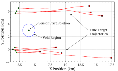
Figure 1: True targets trajectories in scenario 1. Note that the targets appear and disappear at different times, which is not represented on the plot.

To evaluate the control performance, we compare the estimation accuracy under the proposed control scheme, against the case of a stationary sensor, and the case where the sensor performs randomly chosen course changes. For each of the three cases, we have performed 100 Monte Carlo runs, and used a multi-target miss distance known as the optimal sub-pattern assignment (OSPA) metric [66], to quantify the positional error between the filter estimates and the ground truth. Figure 2 shows the average of the OSPA distance versus time where the OSPA cutoff parameter is $c=200\text{m}$ and the order parameter is $p=2$. These results show that the proposed control strategy provides the best estimation performance. In the cases where the sensor is stationary or undergoing randomly chosen actions, the performance is significantly worse, since they have no mechanism for positioning the sensor in the most favourable location. This demonstrates that the use of Cauchy-Schwarz divergence as the reward function has been effective at reducing the estimation error of the system.

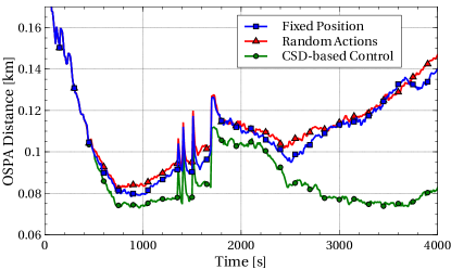
Figure 2: Comparison of OSPA versus time for the cases of fixed sensor location, randomised control actions, and control based on the Cauchy-Schwarz divergence / void probability.

Figure 3 shows a heatmap summarizing the paths taken by the sensor over the 100 Monte Carlo runs. From this diagram, the general trend of the controlled sensor’s trajectory can be observed. Intuition would suggest that the sensor should move closer to the areas with the higher concentration of targets, which agrees with the trend shown in Figure 3.

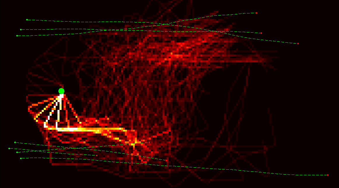
Figure 3: This heatmap shows the sensor location over 100 Monte Carlo runs. Brighter colors represent locations that were more frequently visited. The sensor usually starts by moving towards the four targets at the bottom. After some of those targets become terminated, the sensor moves towards the three targets at the top. A few exceptions to this behaviour can be seen, but the general trend is clearly visible.

To demonstrate the operation of the control scheme, we now show a single run which exhibits the typical control behaviour. We have shown the scenario geometry and expected Cauchy-Schwarz divergence for each potential action at five different time instants; at 400s when the first decision is made (Figure (4)), the third decision at time 1200s (Figure 5), the sixth decision at time 2400s (Figure 6), the eigth decision at time 3200s (Figure 7), and finally, at the end of the scenario at time 4000s (Figure 8).

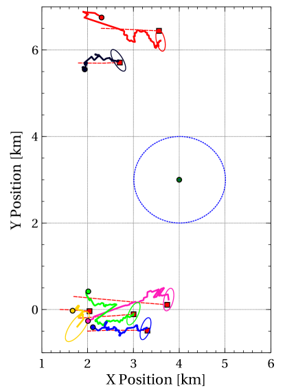
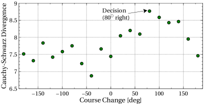
Figure 4: Scenario geometry and reward curve at the time of the first decision (400s). The sensor platform is stationary for the first 400s, and pointing towards the right. The first decision made by the control algorithm is to turn $80^{\circ}$ to the right, which takes the sensor towards the group of four targets.

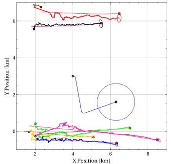
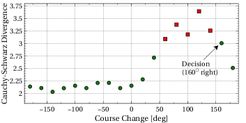
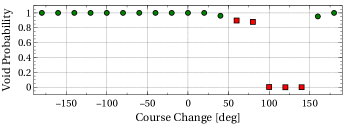
Figure 5: Scenario geometry, reward curve and void probability curve at the time of the third decision (1200s). Four of the manoeuvres do not satisfy the constraint, because they would result in high probability of targets getting too close to the sensor. Excluding these, the best remaining decision is to turn $160^{\circ}$ to the right.

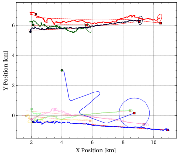
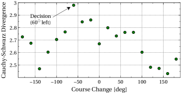
Figure 6: Scenario geometry and reward curve at the time of the sixth decision (2400s). Three of the targets at the bottom have terminated since time 1200s (as indicated by the faint tracks), and one additional target has appeared at the top. As a result, the algorithm decides to turn $60^{\circ}$ left, taking it closer to the three targets at the top.

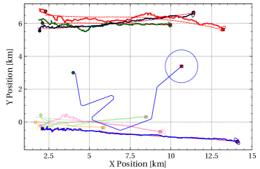
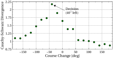
Figure 7: Scenario geometry and reward curve at the time of the eigth decision (3200s). The algorithm decides on a slight turn to the left, which takes it closer to the group of three targets.

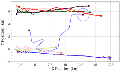
Figure 8: Scenario at time 4000s. The sensor is now following the group of three targets at the top.

IV-F2 Scenario 2

This scenario consists of 8 targets at various locations and moving in different directions, and unlike the previous scenario, the best path for the sensor to take is not immediately obvious. The scenario geometry is shown in Figure 9, which also depicts one of the typical sensor trajectories obtained during the 100 Monte Carlo runs. The starting location for the sensor is fixed near the top right-hand corner for all runs, and in the particular case shown in Figure 9, it moves around the surveillance area, appearing to visit each pair of targets in sequence.

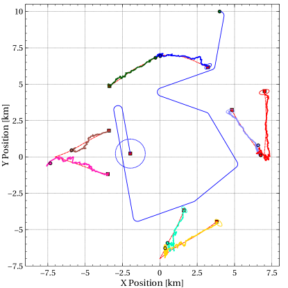
Figure 9: Scenario 2 - Typical sensor trajectory under the proposed control scheme, along with the true and estimated target trajectories.

Figure 10 shows a comparison of the OSPA distance obtained for the cases of fixed sensor location, random actions, and with the proposed control strategy. The sensor with fixed position performs worst, because it has difficulty tracking the targets near the bottom of the surveillance region due to their large distance from the sensor. Moving with randomised actions improves the performance, because despite the randomness of the chosen trajectories, the sensor still has the opportunity to move closer to the far-away targets. The proposed control strategy outperforms both the fixed and randomly moving sensors, as indicated by the lower OSPA distance. Due to the stochastic nature of the problem, the exact behaviour observed in Figure 10 is not necessarily replicated on every run. However the sensor generally moves around the centre of the surveillance region and attempts to visit each target in sequence. This can be observed in Figure 11, which shows that the sensor spends most of the time moving around between the targets.

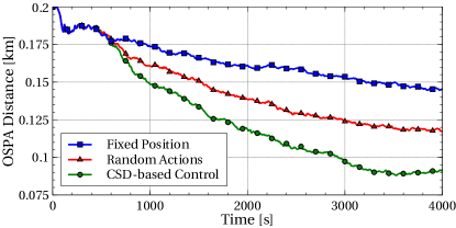
Figure 10: Scenario 2 - Comparison of tracking performance for fixed sensor location, randomly chosen actions, and actions chosen using the Cauchy-Schwarz divergence (CSD) based control scheme.

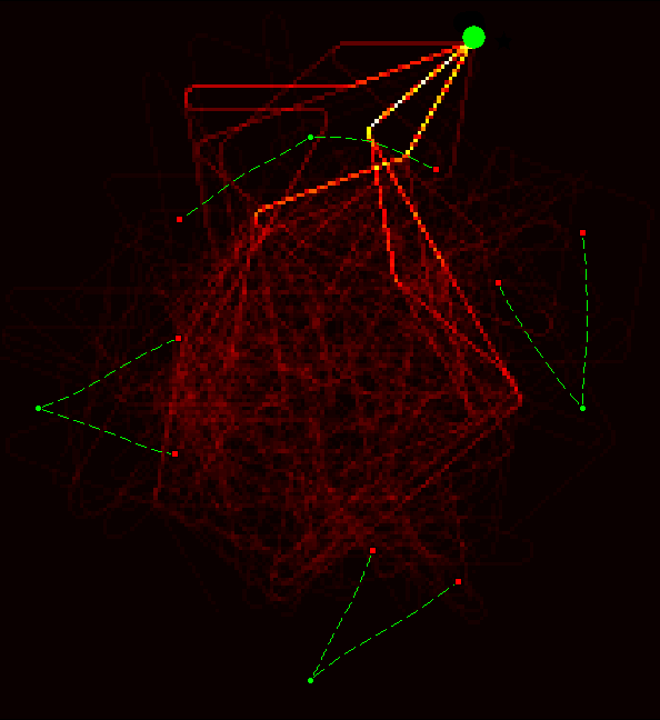
Figure 11: Scenario 2 - Heatmap showing the control behaviour over 100 Monte Carlo runs.

V Conclusion

In this paper we have proposed two useful properties of generalized labeled multi-Bernoulli models; an analytical form for the Cauchy-Schwarz divergence between two GLMBs, and an analytical form for the void probability functional of a GLMB. These properties have applications in areas including GLMB mixture reduction, situational awareness, and sensor management. Here we demonstrated their use in a sensor management application, in which the goal was to plan a sensor trajectory that optimizes the error performance in a multi-target tracking scenario. The problem was formulated as a constrained POMDP, with a reward function based on the expected Cauchy-Schwarz divergence, and a constraint based on the void probability, to ensure adequate separation between the sensor and targets. The results showed that this method was highly effective at reducing the multi-target estimation error, compared to cases where the sensor was stationary or undergoing random actions. This demonstrates that both the proposed Cauchy-Schwarz divergence and void probability functional are versatile tools in multi-object information theory.

References

- [1] D. Daley and D. Vere-Jones, An introduction to the theory of point processes. Springer-Verlag, 1988.
- [2] D. Stoyan, D. Kendall and J. Mecke, Stochastic Geometry and its Applications. John Wiley & Sons, 1995.
- [3] J. Moller and R. Waagepetersen, Statistical Inference and Simulation for Spatial Point Processes. Chapman & Hall CRC, 2004.
- [4] I. Molchanov, Theory of Random Sets, Springer Science & Business Media, 2006.
- [5] A. Baddeley, I. Bárány, R. Schneider, and W. Weil, Stochastic Geometry: Lectures Given at the C.I.M.E. Summer School Held in Martina Franca, Italy, September 13-18, 2004, ser. Lecture Notes in Mathematics / C.I.M.E. Foundation Subseries, Springer, 2007.
- [6] D. Stoyan and A. Penttinen, “Recent applications of point process methods in forestry statistics,” Statistical Science, vol. 15, no. 1, pp. 61-78, 2000.
- [7] Y. Ogata, “Seismicity analysis through point-process modeling: A review,” Pure and Applied Geophysics, vol. 155, no. 2-4, pp. 471-507, 1999.
- [8] V. Marmarelis and T. Berger, “General methodology for nonlinear modeling of neural systems with Poisson point-process inputs,” Mathematical Biosciences, vol. 196, no. 1, pp. 1-13, 2005.
- [9] C. Ji, D. Merl, T. B. Kepler, and M. West, “Spatial mixture modelling for unobserved point processes: Examples in immunofluorescence histology,” Bayesian Analysis, vol. 4, pp. 297-316, 2009.
- [10] D. L. Snyder, L. J. Thomas, and M. M. Ter-Pogossian, “A mathematical model for positron-emission tomography systems having time-of-flight measurements,” IEEE Trans. Nuclear Science, vol. 28, no. 3, pp. 3575-3583, June 1981.
- [11] A. J. Baddeley and M. N. M. Van Lieshout. “Stochastic geometry models in high-level vision,” Jour. of Applied Statistics, vol. 20, no. 5-6, pp. 231-256, 1993.
- [12] R. Hoseinnezhad, B.-N. Vo, B.-T. Vo, and D. Suter, “Visual tracking of numerous targets via multi-Bernoulli filtering of image data,” Pattern Recognition, vol. 45, no. 10, pp. 3625-3635, Oct. 2012.
- [13] F. Baccelli, M. Klein, M. Lebourges, and S. A. Zuyev, “Stochastic geometry and architecture of communication networks,” Telecommunication Systems, vol. 7, no. 1-3, pp. 209-227, 1997.
- [14] M. Haenggi, “On distances in uniformly random networks,” IEEE Trans. Inf. Theory, vol. 51, no. 10, pp. 3584-3586, Oct. 2005.
- [15] M. Haenggi, J. Andrews, F. Baccelli, O. Dousse, and M. Franceschetti, “Stochastic geometry and random graphs for the analysis and design of wireless networks,” IEEE Jour. Selected Areas in Communications, vol. 27, no. 7, pp. 1029-1046, 2009.
- [16] E. Biglieri and M. Lops, “Multiuser detection in a dynamic environment. Part I: User identification and data detection,” IEEE Trans. Inf. Theory, vol. 53, no. 9, pp. 3158-3170, Sep. 2007.
- [17] D. Angelosante, E. Biglieri and M. Lops, “Multiuser detection in a dynamic environment. Part II: Joint user identification and parameter estimation,” IEEE Trans. Inf. Theory, vol. 55, no. 5, pp. 2365-2374, May 2009.
- [18] R. Mahler, “Multitarget Bayes filtering via first-order multitarget moments,” IEEE Trans. Aerosp. Electron. Syst., vol. 39, no. 4, pp. 1152-1178, Oct 2003.
- [19] R. Mahler, Advances in Statistical Multisource-Multitarget Information Fusion, Artech House, 2014.
- [20] J. Kingman, Poisson Processes, ser. Oxford studies in probability, Oxford University Press, 1993.
- [21] T. M. Cover and J. A. Thomas, Elements of Information Theory. New York, NY, USA: Wiley-Interscience, 1991.
- [22] R. P. S. Mahler, “Global posterior densities for sensor management,” in Proc. SPIE, vol. 3365, pp. 252-263, 1998.
- [23] B.-N. Vo, S. Singh, and A. Doucet, “Sequential Monte Carlo methods for multi-target filtering with random finite sets,” IEEE Trans. Aerosp. Electron. Syst., vol. 41, no. 4, pp. 1224-1245, 2005.
- [24] R. Jenssen, D. Erdogmus, K. E. Hild, J. C. Principe, and T. Eltoft, “Optimizing the Cauchy-Schwarz PDF distance for information theoretic, non-parametric clustering,” in Proc. 5th Int. Conf. on Energy Minimization Methods in Computer Vision and Pattern Recognition, pp. 34-45, Berlin, Heidelberg: Springer-Verlag, 2005.
- [25] R. Jenssen, J. C. Principe, D. Erdogmus, and T. Eltoft, “The Cauchy-Schwarz divergence and Parzen windowing: Connections to graph theory and Mercer kernels,” Journal of the Franklin Institute, vol. 343, no. 6, pp. 614-629, 2006.
- [26] R. Mahler, “Multitarget sensor management of dispersed mobile sensors,” in Theory and Algorithms for Cooperative Systems, D. Grundel, R. Murphey, and P. Pardalos, Eds. World Scientific Books, ch. 12, pp. 239-310, 2004.
- [27] B. Ristic and B.-N. Vo, “Sensor control for multi-object state-space estimation using random finite sets,” Automatica, vol. 46, no. 11, pp. 1812-1818, Nov. 2010.
- [28] H. G. Hoang and B. T. Vo, “Sensor management for multi-target tracking via multi-Bernoulli filtering,” Automatica, vol. 50, no. 4, pp. 1135-1142, Apr. 2014.
- [29] H. Hoang, B.-N. Vo, B.-T. Vo, and R. Mahler, “The Cauchy-Schwarz divergence for Poisson point processes,” IEEE Trans. Inf. Theory, vol. 61, no. 8, pp. 4475-4485, Aug. 2015.
- [30] G. Matheron, Random Sets and Integral Geometry, John Wiley & Sons, 1975.
- [31] J. Mullane, B.-N. Vo, M. Adams, and B.-T. Vo, “A random-finite-set approach to Bayesian SLAM,” IEEE Trans. Robotics, vol. 27, no. 2, pp. 268-282, Apr. 2011.
- [32] C.S. Lee, S. Nagappa, N. Palomeras, D.E. Clark, and J. Salvi. “SLAM with SC-PHD filters: An underwater vehicle application,” IEEE Robotics and Automation Magazine, vol. 21, no. 2, pp. 38-45, June 2014.
- [33] H. Deusch, S. Reuter, and K. Dietmayer. “The labeled multi-Bernoulli SLAM filter,” IEEE Signal Processing Letters, vol. 22, no. 10, pp. 1561-1565, Oct. 2015.
- [34] B. Ristic, B.-N. Vo, and D. Clark, “A note on the reward function for PHD filters with sensor control,” IEEE Trans. Aerosp. Electron. Syst., vol. 47, no. 2, pp. 1521-1529, Apr. 2011.
- [35] B.-T. Vo and B.-N. Vo, “Labeled random finite sets and multi-object conjugate priors,” IEEE Trans. Signal Process., vol. 61, no. 13, pp. 3460-3475, July 2013.
- [36] B.-N. Vo, B.-T. Vo, and D. Phung, “Labeled random finite sets and the Bayes multi-target tracking filter,” IEEE Trans. Signal Process., vol. 62, no. 24, pp. 6554-6567, Dec. 2014.
- [37] S. Reuter, B.-T. Vo, B.-N. Vo, and K. Dietmayer, “The labeled multi-Bernoulli filter,” IEEE Trans. Signal Process., vol. 62, no. 12, pp. 3246-3260, June 2014.
- [38] M. Beard, B.-T. Vo, and B.-N. Vo, “Bayesian Multi-target Tracking with Merged Measurements Using Labelled Random Finite Sets,” IEEE Trans. Signal Process., vol. 63, no. 6, pp. 1433-1447, 2015.
- [39] A. K. Gostar, R. Hoseinnezhad, and A. Bab-Hadiashar. “Sensor control for multi-object tracking using labeled multi-Bernoulli filter,” in Proc. 17th Int. Conf. Information Fusion, Salamanca, Spain, July 2014.
- [40] F. Papi and D. Y. Kim. “A Particle Multi-Target Tracker for Superpositional Measurements using Labeled Random Finite Sets,” IEEE Trans. Signal Process., vol. 63, no. 16, pp. 4348-4358, Aug. 2015.
- [41] M. Beard, B.-T. Vo, B.-N. Vo, and S. Arulampalam, “Sensor Control for Multi-target Tracking using Cauchy-Schwarz Divergence,” in Proc. 18th Int. Conf. Information Fusion, Washington DC, USA, July 2015.
- [42] F. Papi, B.-N. Vo, B.-T. Vo, C. Fantacci, and M. Beard, “Generalized labeled multi-Bernoulli approximation of multi-object densities,” to appear IEEE Trans. Signal Process., 2015.
- [43] S. Reuter, Multi-object tracking using random finite sets, PhD Thesis, Ulm University, Faculty of Engineering and Computer Science, 2014.
- [44] B. A. Jones and B.-N. Vo, “A labeled multi-Bernoulli filter for space object tracking,” in 2014 AAS/AIAA Spaceflight Mechanics Meeting , (AAS 15-413, Williamsburg, VA), January 11-15, 2014.
- [45] B. A. Jones, D. S. Bryant, B.-T. Vo, and B.-N. Vo, “Challenges of Multi-Target Tracking for Space Situational Awareness,” in Proc. 18th Int. Conf. Information Fusion, Washington DC, USA, July 2015.
- [46] M. R. Akella and K. T. Alfriend, “Probability of collision between space objects,” Jour. of Guidance, Control, and Dynamics, vol. 23, no. 5, pp. 769-772, 2000.
- [47] C. E. Rasmussen and C. K. I. Williams, Gaussian Processes for Machine Learning, Cambridge, MA, USA: MIT Press, 2005.
- [48] S. S. Singh, N. Kantas, B.-N. Vo, A. Doucet, R. J. Evans, “Simulation-based optimal sensor scheduling with application to observer trajectory planning,” Automatica, vol. 43, no. 5, pp. 817-830, May 2007.
- [49] Z. Tang, U. Ozguner, “Motion planning for multitarget surveillance with mobile sensor agents”, IEEE Trans. Robotics, vol. 21, no. 5, pp. 898-908, Oct. 2005.
- [50] B. Grocholsky, A. Makarenko and H. Durrant-Whyte, “Information-theoretic coordinated control of multiple sensor platforms,” in Proc. IEEE Int. Conf. Robotics and Automation, 2003.
- [51] Y. Oshman, P. Davidson, “Optimization of observer trajectories for bearings-only target localization,” IEEE Trans. Aerosp. Electron. Syst., vol. 35, no. 3, pp. 892-902, July 1999.
- [52] R. Tharmarasa, T. Kirubarajan, M. L. Hernandez, and A. Sinha, “PCRLB-based multisensor array management for multitarget tracking,” IEEE Trans. Aerosp. Electron. Syst., vol. 43, no. 2, pp. 539-555, Apr. 2007.
- [53] M. L. Hernandez, T. Kirubarajan and Y. Bar-Shalom, “Multisensor resource deployment using posterior Cramer-Rao bounds,” IEEE Trans. Aerosp. Electron. Syst., vol. 40, no. 2, pp. 399-416, 2004.
- [54] V. Krishnamurthy and R. J. Evans, “Hidden Markov model multiarm bandits: A methodology for beam scheduling in multitarget tracking,” IEEE Trans. Signal Process., vol. 49, no. 12, pp. 2893-2908, Dec. 2001.
- [55] C. Kreucher, K. Kastella and A. O. Hero III, “Sensor management using an active sensing approach,” Signal Processing, vol. 85, no. 3, pp. 607-624, Mar. 2005.
- [56] D. J. Kershaw, R. J. Evans, “Optimal Waveform Selection for Target Tracking,” IEEE Trans. Inf. Theory, vol. 40, no. 5, pp. 1536–1550, Sep. 1994.
- [57] R. Niu, P. Willett and Y. Bar-Shalom, “Tracking considerations in selection of radar waveform for range and range-rate measurements,” IEEE Trans. Aerosp. Electron. Syst., vol. 38. no. 2, pp. 467-487, Apr. 2002.
- [58] D. P. Bertsakas, Dynamic Programming and Optimal Control, Belmont:Athena Scientific, 1995.
- [59] G. E. Monahan, “A survey of partially observable Markov decision processes: Theory, models and algorithms,” Management Science, vol. 28, no. 1, pp. 1–16, 1982.
- [60] W. S. Lovejoy, “A survey of algorithmic methods for partially observed Markov decision processes,” Annals of Operations Research, vol. 28, pp. 47-66, 1991.
- [61] D. A. Castanon and L. Carin, “Stochastic control theory for sensor management,” In A. O. Hero, D. A. Castanon, D. Cochran, and K. Kastella Eds., Foundations and Applications of Sensor Management, New York: Springer, 2008, ch. 2, pp. 7-32.
- [62] J. D. Isom, S. P. Meyn, R. D. Braatz, “Piecewise Linear Dynamic Programming for Constrained POMDPs,” in Proc. 23rd AAAI Conf. on Artificial Intelligence, 2008.
- [63] A. Undurti, J. P. How. “An online algorithm for constrained POMDPs,” in Proc. 2010 IEEE Int. Conf. Robotics and Automation, pp. 3966-3973, 2010.
- [64] R. Mahler, “Objective functions for Bayesian control-theoretic sensor management, I: Multitarget first-moment approximation,” in Proc. IEEE Aerospace Conference, Mar. 2003.
- [65] G. Casella and C. P. Robert, “Rao-Blackwellisation of sampling schemes,” Biometrika, vol. 83, pp. 81-94, Mar. 1996.
- [66] D. Schumacher, B.-T. Vo, B.-N. Vo, “A consistent metric for performance evaluation of multi-object filters,” IEEE Trans. Signal Process., vol. 56, no. 8, pp. 3447–3457, Aug. 2008.
- [67] V. Krishnamurthy, “Algorithms for optimal scheduling and management of hidden Markov model sensors,” IEEE Trans. Signal Process., vol. 50, no. 6, pp. 1382-1397, June 2002.