Stable wormholes on a noncommutative-geometry background admitting a one-parameter group of conformal motions

Abstract

When Morris and Thorne first proposed the possible existence of traversable wormholes, they adopted the following strategy: maintain complete control over the geometry, thereby leaving open the determination of the stress-energy tensor. In this paper we determine this tensor by starting with a noncommutative-geometry background and assuming that the static and spherically symmetric spacetime admits conformal motions. This had been established in a previous collaboration with Rahaman et al., using a slightly different approach. Accordingly, the main purpose of this paper is to show that the wormhole obtained can be made stable to linearized radial perturbations.

Keywords: wormholes, conformal motion, noncommutative geometry
PAC numbers: 04.20.-q, 04.20.Gz

1 Introduction

Wormholes are handles or tunnels in spacetime that connect different regions of our Universe but may also connect completely different universes. As first proposed by Morris and Thorne [1], wormholes could be actual physical structures suitable for interstellar travel. For the wormhole spacetime they proposed the following static spherically symmetric line element:

$$ds^{2}=-e^{2\Phi(r)}dt^{2}+\frac{dr^{2}}{1-b(r)/r}+r^{2}(d\theta^{2}+\text{sin}^{2}\theta\,d\phi^{2}),$$ (1)

using units in which $c=G=1$. Here $\Phi=\Phi(r)$ is called the redshift function, which must be everywhere finite to avoid an event horizon. The function $b=b(r)$ is called the shape function since it determines the spatial shape of the wormhole when viewed, for example, in an embedding diagram. The spherical surface $r=r_{0}$ is the radius of the throat of the wormhole and must satisfy the following conditions: $b(r_{0})=r_{0}$, $b(r)<r$ for $r>r_{0}$, and $b^{\prime}(r_{0})<1$, usually called the flare-out condition. This condition can only be satisfied by violating the null energy condition, discussed later.

The Einstein field equations in the orthonormal frame $G_{\hat{\mu}\hat{\nu}}=8\pi T_{\hat{\mu}\hat{\nu}}$ yield the following simple interpretation for the components of the stress-energy tensor: $T_{\hat{t}\hat{t}}=\rho(r)$, the energy density, $T_{\hat{r}\hat{r}}=p_{r}(r)$, the radial pressure, and $T_{\hat{\theta}\hat{\theta}}=T_{\hat{\phi}\hat{\phi}}=p_{t}(r)$, the lateral pressure. For the theoretical construction of the wormhole, Morris and Thorne proposed the following strategy: retain complete control over the geometry by specifying the functions $b=b(r)$ and $\Phi=\Phi(r)$ to obtain the desired properties and then manufacture or search the Universe for the materials or fields that yield the required stress-energy tensor.

Researchers have tried various alternate strategies to accomplish this goal, two of which are discussed in this paper. The first, the assumption of a noncommutative-geometry background, is discussed in Sec. 2. The second, the assumption that the static and spherically symmetric spacetime admits a one-parameter group of conformal motions, is discussed in Sec. 3. Taken together, these assumptions produce both the shape and redshift functions and thus a complete wormhole solution.

Some of these ideas have already been considered in Ref. [2], albeit with slightly different assumptions and techniques. What these approaches have in common is a redshift function resulting in a wormhole that is not asymptotically flat. The wormhole material would therefore have to be cut off and joined to an external Schwarzschild vacuum solution. What makes the redshift function unusual is that the cut-off can be chosen in such a way that the junction surface is a boundary surface, that is, a surface having zero surface stresses. The main goal in this paper is to show that the wormhole obtained is thereby stable to linearized radial perturbations.

2 Noncommutative geometry

A particularly useful outcome of string theory is the recognition that coordinates may become noncommutative operators on a $D$-brane [3, 4]. The commutator is $[\textbf{x}^{\mu},\textbf{x}^{\nu}]=i\theta^{\mu\nu}$, where $\theta^{\mu\nu}$ is an antisymmetric matrix. The implication is that noncommutativity replaces point-like structures by smeared objects. (The aim is to eliminate the divergences that normally occur in general relativity.) The smearing effect can be accomplished by using the Gaussian distribution of minimal length $\sqrt{\theta}$ instead of the Dirac delta function [5, 6, 7, 8]. This is also the approach used in Ref. [2]. An equally effective way is to assume that the energy density of the static and spherically symmetric and particle-like gravitational source has the form [9, 10, 11, 12]

$$\rho(r)=\frac{M\sqrt{\theta}}{\pi^{2}(r^{2}+\theta)^{2}}.$$ (2)

Here the mass $M$ is diffused throughout the region of linear dimension $\sqrt{\theta}$ due to the uncertainty. The noncommutative geometry is an intrinsic property of spacetime and does not depend on particular features such as curvature.

2.1 Wormhole structure

The Einstein field equations $G_{\hat{\mu}\hat{\nu}}=8\pi T_{\hat{\mu}\hat{\nu}}$ result in the following forms [1]:

$$\rho(r)=\frac{b^{\prime}}{8\pi r^{2}},$$ (3)

$$p_{r}(r)=\frac{1}{8\pi}\left[-\frac{b}{r^{3}}+2\left(1-\frac{b}{r}\right)\frac{\Phi^{\prime}}{r}\right],$$ (4)

and

$$p_{t}(r)=\frac{1}{8\pi}\left(1-\frac{b}{r}\right)\left[\Phi^{\prime\prime}-\frac{b^{\prime}r-b}{2r(r-b)}\Phi^{\prime}+(\Phi^{\prime})^{2}+\frac{\Phi^{\prime}}{r}-\frac{b^{\prime}r-b}{2r^{2}(r-b)}\right].$$ (5)

Since Eq. (5) can be obtained from the conservation of the stress-energy tensor, $T^{\mu\nu}_{\phantom{\mu\nu};\nu}=0$, only two of Eqs. (3)-(5) are independent. As a result, these can be written in the following form:

$$b^{\prime}=8\pi\rho r^{2},$$ (6)

and

$$\Phi^{\prime}=\frac{8\pi p_{r}r^{3}+b}{2r(r-b)}.$$ (7)

Eq. (2) immediately yields the total mass-energy $M$ of the wormhole inside a sphere of radius $r$:

$$M=\int^{r}_{0}\rho(r^{\prime})4\pi(r^{\prime})^{2}dr^{\prime}=\frac{2M}{\pi}\left(\text{tan}^{-1}\frac{r}{\sqrt{\theta}}-\frac{r\sqrt{\theta}}{r^{2}+\theta}\right).$$ (8)

Next, from Eq. (3),

$$b(r)=\frac{8M\sqrt{\theta}}{\pi}\int^{r}_{r_{0}}\frac{(r^{\prime})^{2}dr^{\prime}}{[(r^{\prime})^{2}+\theta]^{2}}+r_{0},$$ (9)

so that $b(r_{0})=r_{0}$, as required. Since Eq. (9) is valid for any $r_{0}$, the wormhole can be macroscopic. The resulting shape function is

$$b(r)=\frac{4M\sqrt{\theta}}{\pi}\left(\frac{1}{\sqrt{\theta}}\text{tan}^{-1}\frac{r}{\sqrt{\theta}}-\frac{r}{r^{2}+\theta}-\frac{1}{\sqrt{\theta}}\text{tan}^{-1}\frac{r_{0}}{\sqrt{\theta}}+\frac{r_{0}}{r_{0}^{2}+\theta}\right)+r_{0}.$$ (10)

Moreover, from

$$b^{\prime}(r)=\frac{8M\sqrt{\theta}r^{2}}{\pi(r^{2}+\theta)^{2}},$$ (11)

we find that (since $\sqrt{\theta}\ll M$)

$$0<b^{\prime}(r)<1,$$

so that the flare-out condition is met.

Remark: For later use, we observe that $b(r)$ has continuous derivatives of all orders.

2.2 The null energy condition

Closely related to the flare-out condition is the violation of the null energy condition. Observe that

$$\rho(r)+p_{r}(r)=\frac{M\sqrt{\theta}}{\pi^{2}(r^{2}+\theta)^{2}}+\left.\frac{1}{8\pi}\left[-\frac{b}{r^{3}}+2\left(1-\frac{b}{r}\right)\frac{\Phi^{\prime}}{r}\right]\right|_{r=r_{0}}\\ =\frac{M\sqrt{\theta}}{\pi^{2}(r_{0}^{2}+\theta)^{2}}-\frac{1}{8\pi}\frac{b(r_{0})}{r_{0}^{3}}<0$$ (12)

since $\sqrt{\theta}\ll M$. The violation of the null energy condition can be attributed to the noncommutative-geometry background without hypothesizing the need for “exotic matter.”

3 Conformal Killing vectors

We assume in this paper that our static spherically symmetric spacetime admits a one-parameter group of conformal motions. These are motions along which the metric tensor of a spacetime remains invariant up to a scale factor. This assumption is equivalent to the existence of conformal Killing vectors such that

$$\mathcal{L_{\xi}}g_{\mu\nu}=g_{\eta\nu}\,\xi^{\eta}_{\phantom{A};\mu}+g_{\mu\eta}\,\xi^{\eta}_{\phantom{A};\nu}=\psi(r)\,g_{\mu\nu},$$ (13)

where the left-hand side is the Lie derivative of the metric tensor and $\psi(r)$ is the conformal factor. (For further discussion, see [13, 14].) The vector $\xi$ generates the conformal symmetry and the metric tensor $g_{\mu\nu}$ is conformally mapped into itself along $\xi$. According to [15, 16], this type of symmetry has been used effectively to describe relativistic stellar-type objects, not only yielding new solutions, but leading to new geometric and kinematical insights [17, 18, 19, 20].

As already noted, exact solutions of traversable wormholes admitting conformal motions are discussed on Ref. [2]. Two earlier studies assumed non-static conformal symmetry [14, 21].

To study the effect of conformal symmetry, it is convenient to use an alternate form of the metric [2]:

$$ds^{2}=-e^{\nu(r)}dt^{2}+e^{\lambda(r)}dr^{2}+r^{2}(d\theta^{2}+\text{sin}^{2}\theta\,d\phi^{2}).$$ (14)

The Einstein field equations then take on the following form:

$$e^{-\lambda}\left(\frac{\lambda^{\prime}}{r}-\frac{1}{r^{2}}\right)+\frac{1}{r^{2}}=8\pi\rho,$$ (15)

$$e^{-\lambda}\left(\frac{1}{r^{2}}+\frac{\nu^{\prime}}{r}\right)-\frac{1}{r^{2}}=8\pi p_{r},$$ (16)

and

$$\frac{1}{2}e^{-\lambda}\left[\frac{1}{2}(\nu^{\prime})^{2}+\nu^{\prime\prime}-\frac{1}{2}\lambda^{\prime}\nu^{\prime}+\frac{1}{r}({\nu^{\prime}-\lambda^{\prime}})\right]=8\pi p_{t}.$$ (17)

Next, following Herrera and Ponce de León [15], we restrict the vector field by requiring that $\xi^{\alpha}U_{\alpha}=0$, where $U_{\alpha}$ is the four-velocity of the perfect fluid distribution. The assumption of spherical symmetry then implies that $\xi^{0}=\xi^{2}=\xi^{3}=0$ [15]. Eq. (13) now yields the following results:

$$\xi^{1}\nu^{\prime}=\psi,$$ (18)

$$\xi^{1}=\frac{\psi r}{2},$$ (19)

and

$$\xi^{1}\lambda^{\prime}+2\,\xi^{1}_{\phantom{1},1}=\psi.$$ (20)

We can then use these equations to obtain

$$e^{\nu}=Cr^{2}$$ (21)

and

$$e^{\lambda}=\left(\frac{a}{\psi}\right)^{2},$$ (22)

where $C$ and $a$ are integration constants. The Einstein field equations can also be rewritten:

$$\frac{1}{r^{2}}\left(1-\frac{\psi^{2}}{a^{2}}\right)-\frac{2\psi\psi^{\prime}}{a^{2}r}=8\pi\rho,$$ (23)

$$\frac{1}{r^{2}}\left(\frac{3\psi^{2}}{a^{2}}-1\right)=8\pi p_{r},$$ (24)

and

$$\frac{\psi^{2}}{a^{2}r^{2}}+\frac{2\psi\psi^{\prime}}{a^{2}r}=8\pi p_{t}.$$ (25)

As before, only two of Eqs. (23) -(25) are independent.

It is interesting to note that the shape function, Eq. (10), can also be obtained by substituting Eq. (2) into Eq. (23) instead of Eq. (3), as before. So the assumption of conformal symmetry is clearly not needed for determining $b(r)$, but it does determine the redshift function from Eq. (21), thereby completing the wormhole solution. Using the notation in Sec. 1, we therefore have

$$e^{2\Phi}=Cr^{2}\quad\text{and}\quad\Phi=\frac{1}{2}\,\text{ln}\,(Cr^{2}).$$ (26)

It now becomes apparent that our wormhole spacetime is not asymptotically flat. In fact, the redshift function obtained above does not even appear to have a particularly desirable form. It turns out, however, that the form actually has some unexpected and potentially useful properties, as we will see in the next section.

4 Junction to an external vacuum solution

Since by Eq. (21) the wormhole spacetime is not asymptotically flat, the wormhole material must be cut off at some $r=a$ and joined to an exterior Schwarzschild solution,

$$ds^{2}=-\left(1-\frac{2M}{r}\right)dt^{2}+\frac{dr^{2}}{1-2M/r}+r^{2}(d\theta^{2}+\text{sin}^{2}\theta\,d\phi^{2}).$$ (27)

Here $M=\frac{1}{2}b(a)$, so that $e^{2\Phi}=Ca^{2}=1-2M/a$, whence

$$C=\frac{1-2M/a}{a^{2}},$$ (28)

where $M$ is determined from in Eq. (8).

While the metric is now continuous at the junction surface, the derivatives are not. The following forms, proposed by Lobo [22, 23], are suitable for present purposes and will be discussed further in the next section:

$$\sigma=-\frac{1}{4\pi a}\left(\sqrt{1-\frac{2M}{a}}-\sqrt{1-\frac{b(a)}{a}}\right)$$ (29)

and

$$\mathcal{P}=\frac{1}{8\pi a}\left(\frac{1-\frac{M}{a}}{\sqrt{1-\frac{2M}{a}}}-[1+a\Phi^{\prime}(a)]\sqrt{1-\frac{b(a)}{a}}\right).$$ (30)

Since $b(a)=2M$, the surface stress-energy $\sigma$ is zero. From $e^{2\Phi}=Cr^{2}$, we find that $\Phi^{\prime}(a)=1/a$ and $a\Phi^{\prime}(a)=1$. Now Eq. (30) becomes

$$\mathcal{P}=\frac{1}{8\pi a}\left(\frac{1-\frac{M}{a}}{\sqrt{1-\frac{2M}{a}}}-2\sqrt{1-\frac{b(a)}{a}}\right).$$ (31)

Since $b(r)<r$ and $b(r)/r$ is monotone decreasing, we can choose $a$ in such a way that $b(a)/a=2/3$, and since $2M=b(a)$, we get $\mathcal{P}=0$ by Eq. (31).

We conclude that the cut-off can be chosen in such a way that the surface stresses are zero. Such a surface is called a boundary surface and should result in a stable structure. That is the topic of the next section.

5 Stability analysis

Given the junction surface $r=a$, denoted by $S$, our starting point is the Darmois-Israel formalism [24, 25]: if $K_{ij}$ is the extrinsic curvature across $S$ (also known as the second fundamental form), then the stress-energy tensor $S^{i}_{\phantom{i}j}$ is given by the Lanczos equations:

$$S^{i}_{\phantom{i}j}=-\frac{1}{8\pi}\left([K^{i}_{\phantom{i}j}]-\delta^{i}_{\phantom{i}j}[K]\right),$$ (32)

where $[X]=\lim_{r\to a+}X-\lim_{r\to a-}X=X^{+}-X^{-}.$ So $[K_{ij}]=K^{+}_{ij}-K^{-}_{ij},$ which expresses the discontinuity in the second fundamental form, and $[K]$ is the trace of $[K^{i}_{\phantom{i}j}]$.

In terms of the energy-density $\sigma$ and the surface pressure $\mathcal{P}$, $S^{i}_{\phantom{i}j}=\text{diag}(-\sigma,\mathcal{P},\mathcal{P}).$ The Lanczos equations now yield

$$\sigma=-\frac{1}{4\pi}[K^{\theta}_{\phantom{\theta}\theta}]$$ (33)

and

$$\mathcal{P}=\frac{1}{8\pi}\left([K^{\tau}_{\phantom{\tau}\tau}]+[K^{\theta}_{\phantom{\theta}\theta}]\right).$$ (34)

A dynamic analysis can be obtained by letting the radius $r=a$ be a function of time, as in Ref. [26]. Here the overdots denote derivatives with respect to $\tau$. According to Lobo [27], the components of the extrinsic curvature are given by

$$K^{\tau+}_{\phantom{\tau}\tau}=\frac{\frac{M}{a^{2}}+\overset{..}{a}}{\sqrt{1-\frac{2M}{a}+\overset{.}{a}^{2}}},$$ (35)

$$K^{\tau-}_{\phantom{\tau}\tau}=\frac{\Phi^{\prime}\left(1-\frac{b(a)}{a}+\overset{.}{a}^{2}\right)+\overset{..}{a}-\frac{\overset{.}{a}^{2}\left[b(a)-ab^{\prime}(a)\right]}{2a[a-b(a)]}}{\sqrt{1-\frac{b(a)}{a}+\overset{.}{a}^{2}}},$$ (36)

and

$$K^{\theta+}_{\phantom{\theta}\theta}=\frac{1}{a}{\sqrt{1-\frac{2M}{a}+\overset{.}{a}^{2}}},$$ (37)

$$K^{\theta-}_{\phantom{\theta}\theta}=\frac{1}{a}{\sqrt{1-\frac{b(a)}{a}+\overset{.}{a}^{2}}}.$$ (38)

These forms yield

$$\sigma=-\frac{1}{4\pi}(K^{\theta+}_{\phantom{\theta}\theta}-K^{\theta-}_{\phantom{\theta}\theta})=-\frac{1}{4\pi a}\left(\sqrt{1-\frac{2M}{a}+\overset{.}{a}^{2}}-\sqrt{1-\frac{b(a)}{a}+\overset{.}{a}^{2}}\right).$$ (39)

In the static case, that is, when $\overset{.}{a}=\overset{..}{a}=0$, Eq. (39) reduces to Eq. (30).

Again following Lobo [27], rewriting Eq. (39) in the form

$$\sqrt{1-\frac{2M}{a}+\overset{.}{a}^{2}}=\sqrt{1-\frac{b(a)}{a}+\overset{.}{a}^{2}}-4\pi\sigma a$$ (40)

will yield the following equation of motion:

$$\overset{.}{a}^{2}+V(a)=0.$$ (41)

Here $V(a)$ is the potential, which can be put into the following convenient form:

$$V(a)=1-\frac{\frac{1}{2}b(a)+M}{a}-\left(\frac{M-\frac{1}{2}b(a)}{m_{s}}\right)^{2}-\frac{m^{2}_{s}}{4a^{2}}$$ (42)

where $m_{s}=4\pi a^{2}\sigma$ is the mass of the junction surface, normally referred to as a thin shell [27]. This applies only to cases in which $\sigma$ is different from zero.

When linearized around a static solution at $a=a_{0}$, the solution is stable if, and only if, $V(a)$ has a local minimum value of zero at $a=a_{0}$, that is, $V(a_{0})=0$ and $V^{\prime}(a_{0})=0$, and its graph is concave up: $V^{\prime\prime}(a_{0})>0$. According to Ref. [28], for $V(a)$ in Eq. (42), these conditions are met.

Since we are now dealing with a dynamic analysis, we will take $a=a_{0}$ to be the cut-off discussed earlier. Returning to Eqs. (29) and (30), $\sigma(a_{0})=0$ and $\mathcal{P}(a_{0})=0$. Next, consider the “boundary layer” extending from $r=a_{0}$ to $r=a_{0}+\epsilon$, where $\epsilon>0$ is an arbitrary constant. So for $a_{1}$ in the interval $(a_{0},a_{0}+\epsilon)$, $\sigma(a_{1})$ is no longer equal to zero. Being arbitrarily thin, the boundary layer can be viewed as a thin shell separating the interior and exterior solutions. Since the thin shell is not part of the interior solution, we have, as a result,

$$M<\frac{1}{2}b(a_{1})\quad\text{whenever}\quad\sigma(a_{1})<0$$

and

$$M>\frac{1}{2}b(a_{1})\quad\text{whenever}\quad\sigma(a_{1})>0.$$

We are seeking a solution that (1) meets the stability criterion and (2) is arbitrarily close to our solution. This nearby solution should be viewed as a mathematical solution, rather than a physical one.

To construct such a solution, we modify $b=b(r)$ on the interval $(a_{0},a_{0}+\epsilon)$ smoothly, that is, we modify $b(r)$ in such a way that the second derivative remains continuous (referring to the earlier Remark). The modification is shown in Fig. 1: the concave down

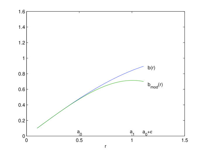
Figure 1: $b^{\prime\prime}(a_{1})<0$ for $a_{1}$ in the interval $(a_{0},a_{0}+\epsilon)$.

curve $b(r)$ is bent down slightly to produce $b^{\prime}_{mod}(a_{1})=0$ for some $a_{1}$ in the interval $(a_{0},a_{0}+\epsilon)$, where $b_{mod}$ denotes the modified shape function. Observe that $b_{mod}$ is also concave down, but it has a larger curvature, that is, $|b^{\prime\prime}(r)|<|b^{\prime\prime}_{mod}(r)|$. Regarding the notation, modifying $b(r)$ will also modify $V(r)$ on the interval $(a_{0},a_{0}+\epsilon)$, denoted by $V_{mod}(r)$. Since our goal is to show that $V^{\prime\prime}(a_{0})>0$ and since $V_{mod}(a_{0})=V(a_{0})$ and $V_{mod}^{\prime\prime}(a_{0})=V^{\prime\prime}_{mod}(a_{0})$, we will retain the original notations $b(r)$ and $V(r)$ to simplify the discussion.

It is important to note that since $\epsilon>0$ can be arbitrarily small, $a_{1}$ is arbitrarily close to $a_{0}$. Moreover, since $\sigma$ is nonzero, $m_{s}=4\pi a_{1}^{2}\sigma$ is also nonzero and, above all, approximately constant. This allows us to find $V^{\prime}$ and $V^{\prime\prime}$ from Eq. (42):

$$V^{\prime}(a_{1})=\frac{d}{da_{1}}\left(-\frac{\frac{1}{2}b(a_{1})+M}{a_{1}}\right)-\frac{2}{m_{s}^{2}}\left(M-\frac{1}{2}b(a_{1})\right)\frac{d}{da_{1}}\left(M-\frac{1}{2}b(a_{1})\right)+\frac{1}{2}\frac{m_{s}^{2}}{a^{3}}$$ (43)

and

$$V^{\prime\prime}(a_{1})=\frac{d^{2}}{da_{1}^{2}}\left(-\frac{\frac{1}{2}b(a_{1})+M}{a_{1}}\right)\\ -\frac{2}{m_{s}^{2}}\left\{\left(M-\frac{1}{2}b(a_{1})\right)\frac{d^{2}}{da_{1}^{2}}\left(M-\frac{1}{2}b(a_{1})\right)+\left[\frac{d}{da_{1}}\left(M-\frac{1}{2}b(a_{1})\right)\right]^{2}\right\}-\frac{3}{2}\frac{m_{s}^{2}}{a^{4}}\\ =-\frac{1}{2}\frac{1}{a_{1}}b^{\prime\prime}(a_{1})+\frac{1}{a_{1}^{2}}b^{\prime}(a_{1})-\frac{1}{a_{1}^{3}}b(a_{1})-\frac{1}{a_{1}^{3}}(2M)\\ -\frac{2}{m_{s}^{2}}\left\{-\frac{1}{2}b^{\prime\prime}(a_{1})\left(M-\frac{1}{2}b(a_{1})\right)+\left[-\frac{1}{2}b^{\prime}(a_{1})\right]^{2}\right\}-\frac{3}{2}\frac{m_{s}^{2}}{a^{4}}.$$ (44)

We would like to determine the conditions for which $V^{\prime\prime}(a_{0})>0$. To that end, we first find the conditions for which

$$V^{\prime\prime}(a_{1})>0.$$ (45)

First observe that $b^{\prime}(a_{1})=0$, $2M\approx b(a_{1})$, while $-(3/2)m_{s}^{2}/a^{4}$ is negligible. This leads to

$$\frac{1}{2}\frac{1}{a_{1}}b^{\prime\prime}(a_{1})<-\frac{1}{a_{1}^{3}}(2b(a_{1}))+\frac{1}{m_{s}^{2}}b^{\prime\prime}(a_{1})\left(M-\frac{1}{2}b(a_{1})\right)$$ (46)

or, after multiplying both sides by $2a_{1}$ and rearranging,

$$\frac{2a_{1}}{m_{s}^{2}}\left(\frac{1}{2}b(a_{1})-M\right)b^{\prime\prime}(a_{1})+b^{\prime\prime}(a_{1})<-\frac{4}{a_{1}^{2}}b(a_{1}).$$ (47)

To satisfy this inequality, the left side must be negative. This implies that we must have $M<\frac{1}{2}b(a_{1})$, so that $\sigma<0$. The need for a negative surface density is consistent with earlier studies involving thin shells [29, 30, 31].) For the critical left-most term, we have from $m_{s}=4\pi a_{1}^{2}\sigma$,

$$\frac{2a_{1}(\frac{1}{2}b(a_{1})-M)b^{\prime\prime}(a_{1})}{[4\pi a_{1}^{2}]^{2}\left(-\frac{1}{4\pi a_{1}}\right)^{2}\left(\sqrt{1-\frac{2M}{a_{1}}}-\sqrt{1-\frac{b(a_{1})}{a_{1}}}\right)\left(\sqrt{1-\frac{2M}{a_{1}}}-\sqrt{1-\frac{b(a_{1})}{a_{1}}}\right)},$$ (48)

which simplifies to

$$\frac{b^{\prime\prime}(a_{1})\left(\sqrt{1-\frac{2M}{a_{1}}}+\sqrt{1-\frac{b(a_{1})}{a_{1}}}\right)}{\sqrt{1-\frac{2M}{a_{1}}}-\sqrt{1-\frac{b(a_{1})}{a_{1}}}}.$$ (49)

This (negative) term becomes arbitrarily large in absolute value as $a_{1}\rightarrow a_{0}$. So reversing the steps, we conclude that sufficiently close to $a=a_{0}$, inequality (47) and hence inequality (45) are satisfied.

Returning to Eq. (42), observe that since $M$ and $m_{s}$ are constants, $V^{\prime\prime}$ is continuous in its domain. Moreover, since $a_{1}$ is arbitrarily close to $a_{0}$, $V^{\prime\prime}(a_{1})>0$ implies that $V^{\prime\prime}(a_{0})>0$: for every $a_{1}$ in the interval $(a_{0},a_{0}+\epsilon)$, there exists $\epsilon_{1}>0$ such that $a_{1}=a_{0}+\epsilon_{1}$. So $V^{\prime\prime}(a_{0}+\epsilon_{1})>0$ implies that $V^{\prime\prime}(a_{0})>0$ because $\lim_{\epsilon_{1}\to 0}V^{\prime\prime}(a_{0}+\epsilon_{1})=V^{\prime\prime}(a_{0})$ by the definition of continuity.

We conclude that our wormhole is stable to linearized radial perturbations.

6 Conclusions

The theoretical construction of Morris-Thorne wormholes is based on the following strategy: retain complete control over the geometry by specifying the redshift and shape functions and then manufacture or search the Universe for materials or fields that produce the required stress-energy tensor. This paper addresses this problem by assuming a noncommutative-geometry background, thereby producing the shape function. The assumption that the spacetime admits a one-parameter group of conformal motions then yields the redshift function. Adding the assumption of the conservation of mass-energy completes the determination of the stress-energy tensor. From a physical standpoint, then, the redshift and shape functions have been determined from the given conditions, rather than simply assigned. The result is a complete wormhole solution.

The resulting wormhole spacetime is not asymptotically flat and has to be cut off and joined to an external vacuum solution at some junction interface. The unusual nature of the redshift function has yielded an unexpected conclusion: the cut-off can be chosen in such a way that the resulting junction surface is a boundary surface, having zero surface stresses. It is subsequently shown that the resulting wormhole has another important physical property: it can be made stable to linearized radial perturbations.

References

- [1] M S Morris and K S Thorne Amer. J. Phys. 56 395 (1988)
- [2] F Rahaman, S Ray, G S Khadekar, P K F Kuhfittig and I Karar Int. J. Theor. Phys. 54 699 (2015)
- [3] E Witten Nucl. Phys. B 460 335 (1996)
- [4] N Seiberg and E Witten J. High Energy Phys. 9909 032 (1999)
- [5] A Smailagic and E Spalluci J. Phys. A 36 L-467 (2003)
- [6] A Smailagic and E Spalluci J. Phys. A 36 L-517 (2003)
- [7] P Nicollini, A Smailagic and E. Spalluci Phys. Lett. B 632 547 (2006)
- [8] P K F Kuhfittig Int. J. Pure Appl. Math. 89 401 (2013)
- [9] J Liang and B Liu Europhys. Lett. 100 30001 (2012)
- [10] K Nozari and S H Mehdipour Class. Quant. Grav. 25 175015 (2008)
- [11] P K F Kuhfittig and Vance D. Gladney J. Mod. Phys. 5 1931 (2014)
- [12] P K F Kuhfittig Int. J. Mod. Phys. D 24 1550023 (2015)
- [13] R Maartens and C M Mellin Class. Quant. Grav. 13 1571 (1996)
- [14] C G Böhmer, T. Harko and F S N Lobo Phys. Rev. D 76 084014 (2007)
- [15] L Herrera and J Ponce de León J. Math. Phys. 26 778 (1985)
- [16] L Herrera and J Ponce de León J. Math. Phys. 26 2018 (1985)
- [17] M Mars and J M M Senovilla Class. Quant. Grav. 10 1633 (1993)
- [18] S Ray, A A Usmani, F Rahaman, M Kalam and K. Chakraborty Ind. J. Phys. 82 1191 (2008)
- [19] F Rahaman, M Jamil, M Kalam, K Chakraborty and A. Ghosh Astrophys. Space Sci. 325 137 (2010)
- [20] F Rahaman, S Ray, I Karar, H I Fatima, S Bhowmick and G.K. Ghosh arXiv: 1211.1228 [gr-qc]
- [21] C G Böhmer, T Harko and F S N Lobo Class. Quant. Grav. 25 075016 (2008)
- [22] F S N Lobo Class. Quant. Grav. 21 4811 (2004)
- [23] F S N Lobo Phys. Rev. D 71 084001 (2005)
- [24] W Israel Nuovo Cimento 44B 1 (1966)
- [25] M Visser Lorentzian Wormholes: From Einstein to Hawking, (New York: American Institute of Physics, 1995), chapter 14.
- [26] E Poisson and M Visser Phys. Rev. D 52 7318 (1995)
- [27] F S N Lobo Phys. Rev. D 71 124022 (2005)
- [28] F S N Lobo and P Crawford Class. Quant. Grav. 22 4869 (2005)
- [29] P K F Kuhfittig AHEP 2012 462493 (2012)
- [30] A A Usmani, Z Hasan, F Rahaman, Sk A Rakib, S Ray and P K F Kuhfittig Gen. Rel. Grav. 42 2901 (2010)
- [31] F Rahaman, K A Rahman, Sk A Rakib and P K F Kuhfittig Int. J. Theor. Phys. 49 2364 (2010) .