Net-proton number kurtosis and skewness in nuclear collisions:
Influence of deuteron formation

Abstract

We explore the influence of deuteron formation in the late stage of nucleus-nucleus reactions on the fluctuations observed in the final net-proton yields around midrapidity. At each investigated energy, the produced (anti-)proton yield at chemical freeze-out is assumed to fluctuate according to a Poisson distribution and in each event the probability for deuteron formation by coalescence is proportional to $(dN_{\mathrm{proton}}/dy)^{2}$. The protons that are then clustered in deuterons are usually not included in the experimental measurement of the net-proton fluctuations, therefore, we subtract these clustered protons from the final state proton number for the calculation of the net-proton fluctuations (the same is done in the anti-proton sector). Due to the non-linear deuteron formation probability the resulting distribution is not a Skellam distribution, but shows the interesting feature of a decrease in the kurtosis $\kappa\sigma^{2}$ and a local maximum in the skewness $S\sigma$ observables as the collision energy decreases.

I Introduction

The exploration of the properties of ultra-hot and super-dense nuclear matter is among the most challenging scientific endeavors today. The collisions of heavy ions allow to explore these properties in the laboratory for the first time with unprecedented precision. Fluctuation observables have gained very great interest in recent years as they may be sensitive to the structure of the QCD phase diagram. In particular they can serve as an indicator for the first order deconfinement phase transition and the associated critical end point Sasaki:2007db ; Randrup:2009gp ; Steinheimer:2012gc ; Stephanov:1999zu . Particle number fluctuations were first explored in experiments at the SPS Alt:2008ab ; Anticic:2008aa . With the availability of the first lattice QCD data on higher order susceptibilities in Allton:2005gk these investigations Stephanov:1998dy ; Stephanov:1999zu ; Jeon:2000wg ; Asakawa:2001mn ; Koch:2001zn ; Koch:2008zz ; Karsch:2010ck have moved to the next level and have been intensively explored with STAR’s Beam Energy Scan (BES) at the RHIC facility Aggarwal:2010wy . Recent results from the BES program indicate a non-trivial beam dependence of the higher order net-baryon number cumulants. This is of particular interest, as these higher order cumulants are very sensitive to the existence of a second order phase transition Stephanov:2008qz ; Koch:2008ia and the associated fluctuations and correlations.

While irregular structures have been observed in the experimental data, the interpretation and final experimental validation are still missing today. For example, effects of conservation laws Schuster:2009jv ; Bzdak:2012an ; Sakaida:2014pya , final state hadronic interactions Kitazawa:2011wh , repulsive hadronic interactions Begun:2012rf and acceptance effects Bzdak:2012ab as well as efficiency corrections Bzdak:2013pha are considered to be very important for the interpretation of experimental results.

It is therefore essential to understand all trivial and non-trivial effects which have an influence on the observed cumulant ratios, in order to make conclusions on the existence and discovery of a phase transition and critical endpoint.

In the following we suggest a further uncertainty, arising from nuclear cluster formation, that needs to be taken into account before final conclusions from these fluctuation observables should be drawn.

II Set-up

For this exploratory study, we will stay with a simple physical picture to elucidate the main effect of cluster production on the observable fluctuations. It is clear that more elaborate studies will be needed to allow for a detailed and more quantitative investigation of the effect of cluster formation.

The scenario is as follows. We assume that the number of chemically frozen out protons in some midrapidity interval $n_{i}$ fluctuates according to a Poisson distribution

$$P_{i}(n_{i})=\lambda_{p}^{n_{i}}\frac{e^{-\lambda_{p}}}{n_{i}!}\,.$$ (1)

Here, $\lambda_{p}$ is the mean number of these initial protons. It is important to realize that after deuteron coalescence some of them will be hidden in deuterons and thus will disappear when counting the observed final state protons. Therefore, $\lambda_{p}$ is unknown at this point but will be determined from the observed proton and deuteron yields later. At higher collision energies a similar procedure should be done for antiprotons. We will show, however, that for the energy range of SPS and below their influence can be neglected.

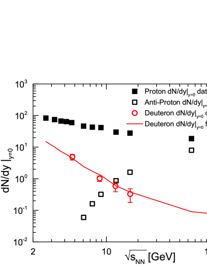
Figure 1: The midrapidity proton, antiproton and deuteron yields from experimental data (symbols) and the corresponding deuteron yield (red solid line) which was extracted using the thermal fit to the $d/p$ ratio, for central Au+Au reactions.

Next, we assume that the probability to form a deuteron by coalescence after the kinetic freeze-out is in each event proportional to the actual initial proton yield squared in that event Butler:1963pp ; Nagle:1996vp , i.e.

$$\lambda_{d}=Bn_{i}^{2}\,,$$ (2)

with a coalescence parameter $B$ which depends only on the beam energy. At this point we make the assumption that the neutron yield in a single event is proportional to the proton yield in that event. If the neutron yield was uncorrelated with the proton number the correlation between proton and deuteron production in a single event is weakened. This feature may be experimentally checked by measuring the production yield of deuterons as a function of the proton number, in a specific centrality bin. Further, it is important to note, that this assumption is only valid in the absence of volume fluctuations. In a scenario where volume fluctuations dominate the observed proton number fluctuations (due to e.g. wide centrality bin selections), both the proton and deuteron number fluctuations will scale with the fluctuations of the volume $n_{i}\propto n_{d}\propto V$. As a result the measured proton number distribution will be described by a Skellam distribution because proton and deuteron fluctuations can be described with independent Poisson distributions. In the case of vanishing volume fluctuations, as is usually ensured by the tight cuts perdormed by the experiments, the deuteron number can be considered correlated with the initial proton number, as presented in eq. (2).

The deuteron yield $n_{d}$ in an event with initial proton multiplicity $n_{i}$ then fluctuates according to a Poisson distribution

$$P_{d}(n_{d}|n_{i})=\lambda_{d}^{n_{d}}\frac{e^{-\lambda_{d}}}{n_{d}!}=\left(Bn_{i}^{2}\right)^{n_{d}}\frac{e^{-Bn_{i}^{2}}}{n_{d}!}\,.$$ (3)

The observed deuteron distribution is obtained by summing over initial proton yields as

$$P_{d}(n_{d})=\sum_{n_{i}}P_{d}(n_{d}|n_{i})P_{i}(n_{i})\,.$$ (4)

To get the observed proton number, we have to subtract from the initial protons those which went into deuterons

$$\frac{dN_{\mathrm{proton}}}{dy}=n_{p}=n_{i}-n_{d}\,.$$ (5)

The distribution of $n_{p}$ then follows from the appropriate convolution of $P_{i}(n_{i})$ with $P_{d}(n_{d}|n_{i})$

$$P(n_{p})=\sum_{n_{i}\geq n_{p}}\sum_{n_{d}}P_{i}(n_{i})P_{d}(n_{d}|n_{i})\delta_{n_{p},n_{i}-n_{d}}\\ =\sum_{n_{i}\geq n_{p}}P_{i}(n_{i})P_{d}(n_{i}-n_{p}|n_{i})\,.$$ (6)

The two parameters in this model are the mean initial proton number $\lambda_{p}$ and the coalescence factor $B$. They can be fixed from the mean observed proton multiplicity and the mean observed deuteron multiplicity

$$\langle n_{p}\rangle = \sum_{n_{p}}n_{p}P(n_{p})$$ (7)

$$\langle n_{d}\rangle = \sum_{n_{d}}n_{d}P_{d}(n_{d})\,,$$ (8)

where $P(n_{p})$ and $P_{d}(n_{d})$ are determined in eqs. (6) and (4).

Then, the distribution $P(n_{p})$ can be used to calculate any moments of the proton distribution.

As the data on deuteron multiplicities for various collision energies are scarce, we note that those that are available are actually well fitted by the thermal model. The deuteron-to-proton multiplicity ratio at midrapidity can be parametrized as

$$\frac{d}{p}=0.8\left[\frac{\sqrt{s_{NN}}}{1\,\mathrm{GeV}}\right]^{-1.55}+0.0036\,,$$

as shown in Andronic:2005yp . Figure 1 depicts the midrapidity proton anti-proton and deuteron yields from experimental data (see Andronic:2005yp and references therein) and the thermal model parametrization of the deuteron yield Andronic:2010qu which serve as input for our calculations.

Using this input we calculate the variance $\sigma$, skewness $S$ and the kurtosis $\kappa$ from the distribution $P(n_{p})$

$$\sigma^{2} = \left\langle(n_{p}-\langle n_{p}\rangle)^{2}\right\rangle$$ (9)

$$S = \frac{\left\langle(n_{p}-\langle n_{p}\rangle)^{3}\right\rangle}{\sigma^{3}}$$ (10)

$$\kappa = \frac{\left\langle(n_{p}-\langle n_{p}\rangle)^{4}\right\rangle}{\sigma^{4}}-3\,.$$ (11)

III Analytic Results

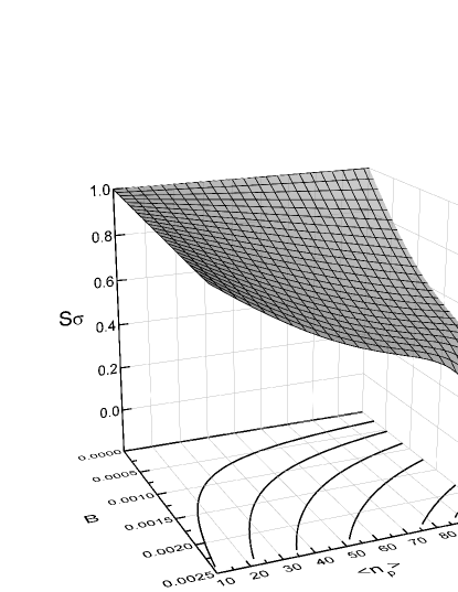
Figure 2: Scaled skewness $S\sigma$ as a function of the mean observed proton number and the coalescence parameter $B$ in the region of values relevant for AGS and SPS collision energies.

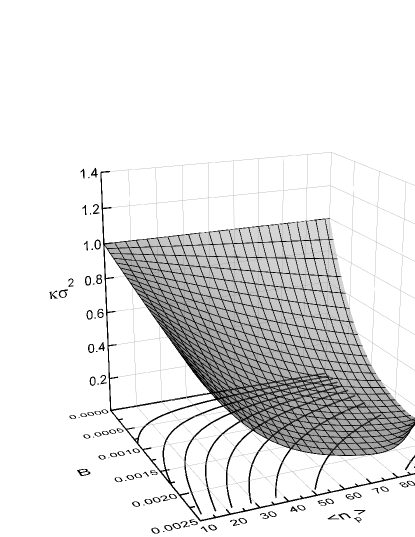
Figure 3: Same as Fig. 2 but for the scaled kurtosis $\kappa\sigma^{2}$.

For illustration, in Fig. 2 we show the scaled skewness $S\sigma$ and in Fig. 3 the scaled kurtosis $\kappa\sigma^{2}$ of the distribution $P(n_{p})$ as functions of the observed mean proton number $\langle n_{p}\rangle$ and the coalescence parameter $B$.

Recall that both $S\sigma$ and $\kappa\sigma^{2}$ would be equal to unity if the underlying observed proton distribution was Poissonian. (There is deviation from 1 for $S\sigma$ if the distribution was Skellam, but we will scale it out later in the presentation of results.) This is really so in the absence of deuterons, i.e. when $B=0$ or for small numbers of observed protons.

We also see a strong deviation from unity for large values of $\langle n_{p}\rangle$ and $B$. In fact the scaled kurtosis may take values which are both smaller or larger than unity.

For a medium value of proton multiplicity and/or coalescence parameter the obtained deuteron number limits the possible observed proton number fluctuation. Since the mean deuteron number scales with the square of proton number, if the proton number becomes large in an event, the number of deuterons makes even larger relative deviation from the mean. This limits the fluctuations of the observed protons mainly on the upper side of the distribution and the tails of the distribution are below a comparable Poisson distribution. When the deuteron number grows further, it starts pushing the observed proton number down (in agreement with eq. (5)). This increases the deviations of the proton number from the mean to lower values. The left tail of the distribution is above Poissonian and the kurtosis grows. The skewness becomes clearly smaller.

Figure 4 shows the results for the beam energy dependence of the scaled skewness and kurtosis, using as input measured mid-rapidity yields of protons and deuterons. We observe a clear deviation from unity for all beam energies under consideration.

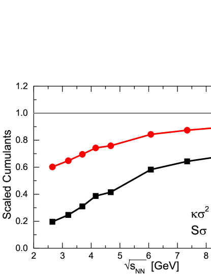
Figure 4: Analytic results for the skewness and kurtosis for Au+Au collisions in the energy range where antiproton production is not important.

IV Results including anti-protons

In order to extend our investigations to beam energies higher than $\sqrt{s_{NN}}\approx 10$ GeV, we need to include the effects of anti-protons and anti-deuterons into our study. This extension of our approach is straightforward. As the measured mean proton and anti-proton numbers are known we can assume that both the proton and anti-proton number separately follow a Poisson distribution. From this assumption, the initial proton and anti-proton number can be sampled independently and according to their measured multiplicities, as described in the previous section. Since the fluctuations of both are described by uncorrelated Poisson distributions the fluctuations of the initial net-proton number should be described by a Skellam distribution. Assuming that the coalescence parameter for anti-deuterons is identical to that of deuteron formation we can numerically determine the final net-proton number in a given event as

$$n_{p-\overline{p}}=(n_{i}-n_{d})-(n_{\overline{i}}-n_{\overline{d}})\mathrm{,}$$ (12)

as well as the corresponding net-proton number distributions. To obtain the mean final net-proton number and its cumulants we perform a numerical sampling of the initial proton and anti-proton number as well as the coresponding (anti-)deuteron numbers in each event. To achieve satisfactory statistics we sample $10^{9}$ events per beam energy. The resulting scaled cumulants of the proton number distributions, $S\sigma$ and $\kappa\sigma^{2}$, are shown in Fig. 5 as functions of energy for central Au+Au reactions over a broad range of energies. We compare our numerical results including anti-protons and anti-deuterons with the analytical results obtained in the previous section. For the lower SPS energies only small variations are observed. We clearly confirm the drastic deviation from the expectation of a Poisson or Skellam distribution. The $\kappa\sigma^{2}$ and $S\sigma$ show strong deviations from unity as the energy decreases and the deuteron fraction increases. This indicates that the formation of deuterons after the kinetic freeze-out may lead to substantial modifications of the fluctuation observable considered here.

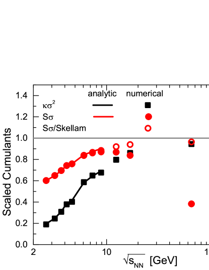
Figure 5: The quantities $S\sigma$ and $\kappa\sigma^{2}$ as functions of energy for central Au+Au reactions over a broad range of energies. Compared are the numerical and analytic results. We clearly observe a drastic deviation from the expectation of a Poisson or Skellam distribution.

V Summary

In the light of the ongoing debate on the interpretation of the recently and currently measured data on fluctuations, we have explored the influence of deuteron formation on fluctuation observables. We employed a standard approach and used that the deuteron formation probability is proportional to the square of the proton yield. This non-linear coupling of the proton and deuteron yields results in a substantial modification of the fluctuation patterns towards low energies: a strong reduction of the $\kappa\sigma^{2}$ and $S\sigma/$Skellam observable has been found.

- (1) C. Sasaki, B. Friman and K. Redlich, Phys. Rev. Lett. 99, 232301 (2007)
- (2) J. Randrup, Phys. Rev. C 79, 054911 (2009)
- (3) J. Steinheimer and J. Randrup, Phys. Rev. Lett. 109, 212301 (2012)
- (4) M. A. Stephanov, K. Rajagopal and E. V. Shuryak, Phys. Rev. D 60, 114028 (1999)
- (5) C. Alt et al. [NA49 Collaboration], Phys. Rev. C 79, 044910 (2009)
- (6) T. Anticic et al. [NA49 Collaboration], Phys. Rev. C 79, 044904 (2009)
- (7) C. R. Allton et al., Phys. Rev. D 71, 054508 (2005)
- (8) M. A. Stephanov, K. Rajagopal and E. V. Shuryak, Phys. Rev. Lett. 81, 4816 (1998)
- (9) S. Jeon and V. Koch, Phys. Rev. Lett. 85, 2076 (2000)
- (10) M. Asakawa, U. W. Heinz and B. Muller, Nucl. Phys. A 698, 519 (2002)
- (11) V. Koch, M. Bleicher and S. Jeon, Nucl. Phys. A 698, 261 (2002) [Nucl. Phys. A 702, 291 (2002)]
- (12) V. Koch, J. Phys. G35, 104030 (2008).
- (13) F. Karsch and K. Redlich, Phys. Lett. B 695, 136 (2011)
- (14) M. M. Aggarwal et al. [STAR Collaboration], Phys. Rev. Lett. 105, 022302 (2010)
- (15) M. A. Stephanov, Phys. Rev. Lett. 102, 032301 (2009)
- (16) V. Koch, arXiv:0810.2520 [nucl-th].
- (17) M. Nahrgang, T. Schuster, R. Stock, M. Mitrovski and M. Bleicher, Eur. Phys. J. C 72, 2143 (2012)
- (18) A. Bzdak, V. Koch and V. Skokov, Phys. Rev. C 87, 014901 (2013)
- (19) M. Sakaida, M. Asakawa and M. Kitazawa, Phys. Rev. C 90, no. 6, 064911 (2014).
- (20) M. Kitazawa and M. Asakawa, Phys. Rev. C 85, 021901 (2012)
- (21) V. V. Begun, M. Gazdzicki and M. I. Gorenstein, arXiv:1208.4107 [nucl-th].
- (22) A. Bzdak and V. Koch, Phys. Rev. C 86, 044904 (2012)
- (23) A. Bzdak and V. Koch, Phys. Rev. C 91, no. 2, 027901 (2015).
- (24) S. T. Butler and C. A. Pearson, Phys. Rev. 129, 836 (1963).
- (25) J. L. Nagle, B. S. Kumar, D. Kusnezov, H. Sorge and R. Mattiello, Phys. Rev. C 53, 367 (1996).
- (26) A. Andronic, P. Braun-Munzinger and J. Stachel, Nucl. Phys. A 772, 167 (2006)
- (27) A. Andronic, P. Braun-Munzinger, J. Stachel and H. Stocker, Phys. Lett. B 697, 203 (2011)