Radiation Gauge in AdS/QCD: inadmissibility and implications on spectral functions in the deconfined phase

Abstract

We point out a subtlety in choosing the radiation gauge ($A_{z}=0$ combined with the Lorenz gauge) for gauge fields in AdS/QCD for black hole backgrounds. We then demonstrate the effect of this on the momentum-dependence of the spectral functions of the $J/\psi$ vector meson, showing a spreading with momentum and a breaking of isotropy, in contrast to previous results in the literature. We also discuss the dependence on a background magnetic field, following our earlier proposed model.

I Introduction

In this note, we would like to discuss in detail the choice of the radiation gauge as it is frequently applied in holographic approaches to QCD. Our specific interest arose from the soft wall model, but the arguments given in the next section do apply to any gauge field in an AdS or AdS black hole background.

In the soft wall model, one studies excitations of a gauge field in AdS with action

$$S=-\frac{1}{4g_{5}^{2}}\int d^{5}x\sqrt{-g}e^{-\Phi}\text{tr}\left[F^{L,MN}F_{L,MN}+F^{R,MN}F_{R,MN}\right],$$ (1)

for left and right gauge fields $A_{L}$ and $A_{R}$. We will denote 5-dimensional indices as $M,N,O,P$ and 4-dimensional (boundary) indices with $\mu,\nu$. The corresponding equations of motion of either gauge field are given by:

$$\partial_{M}\left(e^{-\Phi}\sqrt{-G}G^{MO}G^{NP}(\partial_{O}A_{P}-\partial_{P}A_{O})\right)=0,$$ (2)

where the background geometry is either AdS:

$$ds^{2} =\frac{L^{2}}{z^{2}}\left(-dt^{2}+d\mathbf{x}^{2}+dz^{2}\right)\,,\qquad e^{-\Phi}=e^{-cz^{2}},$$ (3)

or the AdS black hole:

$$ds^{2} =\frac{L^{2}}{z^{2}}\left(-f(z)dt^{2}+d\mathbf{x}^{2}+\frac{dz^{2}}{f(z)}\right)\,,\qquad e^{-\Phi}=e^{-cz^{2}},$$ (4)

with $f(z)=1-z^{4}/z_{h}^{4}$ and $z=z_{h}$ the horizon location. The background includes a dilaton field $\Phi$ whose backreaction on the geometry is assumed to be minor. This model gained popularity to holographically capture important QCD physics, e.g. because of its correct scaling behavior of the meson spectrum and the reader is referred elsewhere for more motivation and details of this model Erlich:2005qh ; Karch:2006pv ; Karch:2010eg .

As a particular example where the soft model was used to study strongly coupled QCD physics, let us refer to Fujita:2009wc ; Fujita:2009ca where heavy quarkonia were studied. The authors of Fujita:2009wc ; Fujita:2009ca suggested choosing a flavor-dependent soft-wall parameter $c$, where the light quarks ($u$, $d$, $s$) are combined into a $SU(3)_{L}\times SU(3)_{R}$ soft wall model and the heavy quark of interest (charm in our case) is treated on its own in a $U(1)_{L}\times U(1)_{R}$ Abelian model:

$$S=-\int d^{5}x\sqrt{-g}~{}\text{tr}~{}e^{-c_{\rho}z^{2}}\mathcal{L}_{light}+e^{-c_{J/\psi}z^{2}}\mathcal{L}_{charm}.$$ (5)

Our goal in this work is to compute the momentum-dependence of the $\bar{c}c$ spectral function in this model and to demonstrate that one of the conclusions of Fujita:2009wc ; Fujita:2009ca , namely that isotropy (rotational invariance) is present in the spectral function, is actually a consequence of a forbidden choice of gauge.

II Survey of the radiation gauge in AdS/CFT

The field $A^{\mu}$ has of course a large gauge redundancy and we will investigate here whether the radiation gauge can always be imposed to begin with. The authors of Erlich:2005qh ; Karch:2006pv and Fujita:2009wc ; Fujita:2009ca impose the gauge choice

$$A_{z}=0,\quad\partial^{\mu}A_{\mu}=0,$$ (6)

where $\mu=0,1,2,3$, the transverse indices. We first note that, for a diagonal metric that is only warped in the $z$-direction, one readily finds that

$$\nabla_{\mu}A^{\mu}=\frac{1}{\sqrt{-G}}\partial_{\mu}\left(\sqrt{-G}A^{\mu}\right)=\partial_{\mu}A^{\mu}=\partial^{\mu}A_{\mu},$$ (7)

and hence there is no difference between covariant derivatives and ordinary partial derivatives when computing the divergence of $A^{\mu}$.

The main discussion we want to start here is: can this gauge be chosen in the first place?
Without loss of generality, we may consider a two-step process to get there.

II.1 Step 1

First let $\tilde{A}_{M}=A_{M}+\partial_{M}\chi_{1}$. We choose $\chi_{1}$ such that

$$\chi_{1}=-\int dzA_{z},$$ (8)

which eliminates $\tilde{A}_{z}$. In general this $\chi_{1}$ depends on all 5 coordinates.

II.2 Step 2

Next we perform a second gauge transformation $\tilde{\tilde{A}}_{M}=\tilde{A}_{M}+\partial_{M}\chi_{2}$. Since we want to maintain $\tilde{\tilde{A}}_{z}=0$, we should have $\partial_{z}\chi_{2}=0$. Additionally, we want to impose the Lorenz (Landau) gauge in the transverse (4d) dimensions. This can be done by solving the following wave equation for $\chi_{2}$:

$$\partial^{\mu}\tilde{A}_{\mu}=-\partial^{\mu}\partial_{\mu}\chi_{2}.$$ (9)

In terms of ordinary coordinate partial derivatives we have

$$G^{\mu\nu}\partial_{\nu}\tilde{A}_{\mu}=-G^{\mu\nu}\partial_{\nu}\partial_{\mu}\chi_{2}.$$ (10)

The tricky part is that this metric still depends on $z$. But we just established that $\chi_{2}$ does not! In general this equation is hence unsolvable.

Before delving into a more detailed exposition, let us look at an analogous problem in (3+1)d classical electrodynamics: we are inclined to choose the temporal and Coulomb gauge simultaneously (thereby defining the radiation gauge): $A_{0}=0$ and $\partial_{i}A_{i}=0$. The latter leads to the equation for $\chi_{2}$:

$$\partial_{i}A_{i}=-\partial_{i}^{2}\chi_{2},$$ (11)

for time-independent $\chi_{2}$. This equation is nevertheless solvable: in spite of the time dependence of $A_{i}$ itself, it holds that

$$\partial_{t}\partial_{i}A_{i}=\partial_{i}E_{i}=0,$$ (12)

by virtue of Gauss’ law. The above gauge is hence possible by imposing the (sourceless) Maxwell equations. Though, in the presence of sources, the radiation gauge is inadmissible.

In our case, we are interested in the analogous problem of a sourcefree Maxwell field, but this time in a curved background.
Maxwell’s equations take the form

$$\partial_{M}\left(e^{-\Phi}\sqrt{-G}G^{MO}G^{NP}(\partial_{O}A_{P}-\partial_{P}A_{O})\right)=0.$$ (13)

In the gauge $A_{z}=0$, we consider the $N=z$ component of this equation. For a diagonal metric whose components are independent of $0,1,2,3$, we obtain

$$G^{\mu\nu}\partial_{z}\partial_{\mu}\tilde{A}_{\nu}=0.$$ (14)

Taking then the $z$-derivative of (10), we obtain

$$(\partial_{z}G^{\mu\nu})\partial_{\nu}\tilde{A}_{\mu}=-(\partial_{z}G^{\mu\nu})\partial_{\nu}\partial_{\mu}\chi_{2}.$$ (15)

In the particular case of a metric for which all components have the same $z$-dependence, we can factor out all $z$-dependence, and rewrite the above as

$$\hat{G}^{\mu\nu}\partial_{\nu}\tilde{A}_{\mu}=-\hat{G}^{\mu\nu}\partial_{\nu}\partial_{\mu}\chi_{2},$$ (16)

where $\hat{G}$ is independent of $z$. Even though $\tilde{A}$ depends on $z$, the constraint (14) implies the left hand side is $z$-independent, just as the right hand side. No problems occur and a solution of the above equation in terms of $\chi_{2}$ is possible. This is the case for AdS spacetimes (3).

For the AdS black hole (4), the metric has a different $z$-dependence for the $G_{00}$ component compared to the other components. For such a space, we can write equation (10) as

$$G^{00}\partial_{0}\tilde{A}_{0}+G^{ii}\partial_{i}\tilde{A}_{i}=-G^{00}\partial_{0}\partial_{0}\chi_{2}-G^{ii}\partial_{i}\partial_{i}\chi_{2}.$$ (17)

Dividing by $G^{00}$ and differentiating w.r.t. $z$ we obtain

$$\partial_{z}\partial_{0}\tilde{A}_{0}+\partial_{z}\left(\frac{G^{ii}}{G^{00}}\right)\partial_{i}\tilde{A}_{i}+\frac{G^{ii}}{G^{00}}\partial_{z}\partial_{i}\tilde{A}_{i}=-\partial_{z}\left(\frac{G^{ii}}{G^{00}}\right)\partial_{i}\partial_{i}\chi_{2}.$$ (18)

The constraint (14) for this case reduces to

$$G^{00}\partial_{z}\partial_{0}\tilde{A}_{0}+G^{ii}\partial_{z}\partial_{i}\tilde{A}_{i}=0,$$ (19)

which simplifies equation (18) and yields

$$\partial_{i}\tilde{A}_{i}=-\partial_{i}\partial_{i}\chi_{2},$$ (20)

which is impossible to satisfy since $\partial_{i}\tilde{A}_{i}$ is $z$-dependent in general, unlike the right hand side.

We are thus forced to conclude that the radiation gauge choice is impossible to implement for the AdS black hole. For a non-exhaustive list of instances where such has been done, we refer to Fujita:2009wc ; Fujita:2009ca ; Grigoryan:2010pj ; Cui:2011ag ; He:2013qq ; Hohler:2013vca ; Yang:2015aia .

III Example wherein the inadmissable radiation gauge affects the physical prediction

The gauge choice issue that we highlighted in the previous section, is relevant for the momentum dependence of the spectral functions. From the latter quantity, we can infer information on the melting behavior of the quarkonium in the plasma. Meson melting in a holographic context was also considered in e.g. Fujita:2009wc ; Fujita:2009ca ; Peeters:2006iu ; Ishii:2014paa ; Ali-Akbari:2014gia , and holographic quarkonia in Fujita:2009wc ; Fujita:2009ca ; Hohler:2013vca ; Grigoryan:2010pj ; Hong:2003jm ; Kim:2007rt ; Hou:2007uk . In Fujita:2009ca it was argued that, even though a spatial momentum breaks isotropy, the spectral functions still are, quite miraculously, isotropic. We will demonstrate that this actually arises due to the faulty choice of gauge: if one does not make the additional gauge choice $\partial^{\mu}A_{\mu}=0$, then isotropy is broken as it would be expected when momentum is inserted.

Our main interest here is on the charmonium bound state where we focus on the vector modes ($A_{L}=A_{R}$). To start, one makes the Ansatz $A_{\mu}\sim e^{i\mathbf{k}\cdot\mathbf{x}-i\omega t}$ for the dependence on the boundary coordinates. We will choose $\mathbf{k}$ along the 3-axis.
If one includes spatial momentum into the spectral functions, the transverse polarization differential equation for $A_{1}$ becomes

$$\partial^{2}_{z}A_{1}+\partial_{z}\left(\ln\left(\sqrt{-\mathcal{G}}e^{-cz^{2}}G^{zz}G^{11}\right)\right)\partial_{z}A_{1}-\frac{1}{G^{zz}}\left(G^{tt}\omega^{2}+k^{2}G^{33}\right)A_{1}=0,$$ (21)

where the metric of the black hole (4) is to be used. This ODE can be readily solved numerically using the same methods as in Fujita:2009wc ; Fujita:2009ca ; Dudal:2014jfa . We will present the results further on.

The $A_{3}$ polarization on the other hand becomes much more intricate: it couples directly to $A_{0}$ and one hence needs to solve a coupled system of differential equations. These are given by

$$\partial^{2}_{z}A_{0}+\partial_{z}\ln\left|e^{-\phi}\sqrt{-\mathcal{G}}G^{zz}G^{00}\right|\partial_{z}A_{0}-\frac{G^{33}}{G^{zz}}\left(k^{2}A_{0}+k\omega A_{3}\right)=0,$$ (22)

and

$$\partial^{2}_{z}A_{3}+\partial_{z}\ln\left|e^{-\phi}\sqrt{-\mathcal{G}}G^{zz}G^{33}\right|\partial_{z}A_{3}-\frac{G^{00}}{G^{zz}}\left(\omega^{2}A_{3}+k\omega A_{0}\right)=0.$$ (23)

One readily finds that the combined equation to be solved equals

$$\partial_{z}\left(\frac{G^{zz}}{G^{33}}\partial^{2}_{z}A_{0}\right) +\partial_{z}\left(\frac{G^{zz}}{G^{33}}\partial_{z}\ln\left|e^{-cz^{2}}\sqrt{-\mathcal{G}}G^{zz}G^{00}\right|\partial_{z}A_{0}\right)-k^{2}\partial_{z}A_{0}-\omega^{2}\frac{G^{00}}{G^{33}}\partial_{z}A_{0}=0.$$ (24)

This is a second order differential equation for $V=\partial_{z}A_{0}$. A Frobenius analysis yields the following asymptotic behavior of $V$. For $z\approx 0$, one finds for the two independent solutions $\Phi_{1}$ and $\Phi_{2}$:

$$\Phi_{1}(\epsilon) =\epsilon,\quad\Phi_{1}^{\prime}(\epsilon)=1,$$ (25)

$$\Phi_{2}(\epsilon) =\epsilon\ln(\epsilon),\quad\Phi_{2}^{\prime}(\epsilon)=1+\ln(\epsilon).$$ (26)

For $z\approx z_{h}$, one finds

$$\phi_{\pm}\sim\left(1-\frac{\xi}{\xi_{h}}\right)^{\pm i\omega\xi_{h}/4}.$$ (27)

With these boundary values, one can solve the differential equation for $V$ from the boundary $z=0$ to the horizon $z=z_{h}$.
Following the real-time dictionary Son:2002sd ; Policastro:2002se , see also Teaney:2006nc ; Skenderis:2008dh ; Skenderis:2008dg ; Lindgren:2015lia , a linear combination of $\Phi_{1}$ and $\Phi_{2}$ has to be taken to satisfy ingoing boundary conditions at the horizon. We parameterize this $V$ as

$$V(z)=C(\Phi_{1}+B\Phi_{2}),$$ (28)

in terms of two complex numbers $C$ and $B$. With this solution for $V$, the spectral function can be distilled as follows. Evaluating (22) near the boundary, one finds

$$\partial_{z}V(\epsilon)-\frac{1}{z}V(\epsilon)+k^{2}A_{0}(\epsilon)+k\omega A_{3}(\epsilon)=0,$$ (29)

or with the above form of $V$:

$$C(1+B(1+\ln(\epsilon)))-\frac{1}{\epsilon}C(\epsilon+B\epsilon\ln(\epsilon))+k^{2}A_{0}(\epsilon)+k\omega A_{3}(\epsilon)=0,$$ (30)

yielding

$$C=\frac{k^{2}A_{0}(\epsilon)+k\omega A_{3}(\epsilon)}{B}.$$ (31)

The coupled differential equation leads to three correlators: $\left\langle J_{0}J_{0}\right\rangle$, $\left\langle J_{0}J_{3}\right\rangle$ and $\left\langle J_{3}J_{3}\right\rangle$ where the currents are the charm vector currents. For instance, in evaluating the spectral function for $A_{0}$, one needs to evaluate the combination Son:2002sd ; Policastro:2002se

$$D_{R}(\omega,k)\sim\lim_{z\to 0}\frac{A_{0}\partial_{z}A_{0}}{z}$$ (32)

to obtain the retarded Green function, from which follows the spectral function as

$$\rho(\omega,k)=-\frac{1}{\pi}\Im D_{R}(\omega,k).$$ (33)

We therefore look at

$$-\lim_{z\to 0}\frac{A_{0}\partial_{z}A_{0}}{z}$$ (34)

and functionally differentiate it w.r.t. the boundary value of $A_{0}$ twice. This equals

$$-\frac{A_{0}(\epsilon)\frac{k^{2}A_{0}(\epsilon)}{B}(\epsilon+B\epsilon\ln(\epsilon))}{\epsilon}=-A_{0}(\epsilon)A_{0}(\epsilon)\frac{k^{2}}{B}(1+B\ln(\epsilon))=-A_{0}(\epsilon)A_{0}(\epsilon)\left(\frac{k^{2}}{B}+k^{2}\ln(\epsilon)\right).$$ (35)

The second term can be renormalized by introduction of a local counterterm (cf. holographic renormalization).

One can also look at the $A_{3}A_{0}$ correlator, though we will have no interest in this mixed correlator in this work.

Finally, we can also look at the $A_{3}A_{3}$ correlator. The correlator can in this case be distilled as (using $\omega G^{00}\partial_{z}A_{0}=kG^{33}\partial_{z}A_{3}$)

$$\frac{A_{3}(\epsilon)\partial_{z}A_{3}}{\epsilon}=-A_{3}(\epsilon)\frac{\omega\partial_{z}A_{0}(\epsilon)}{k\epsilon}=-\frac{A_{3}(\epsilon)A_{3}(\epsilon)\omega k\omega}{kB\epsilon}(\epsilon+B\epsilon\ln(\epsilon))=-A_{3}(\epsilon)A_{3}(\epsilon)\left(\frac{\omega^{2}}{B}+\omega^{2}\ln(\epsilon)\right),$$ (36)

so for the spectral function, it turns out we should look at $-\Im\frac{\omega^{2}}{B}$. It is this correlator that we will be interested in in the remainder of this work.

III.1 Results

Below are the resulting Figures of the spectral functions as $k$ is varied for the two different polarizations. We denote everything in dimensionless quantities (by rescaling $z$) where in particular

$$\xi=\sqrt{c}z,\quad\tilde{\omega}=\frac{\omega}{\sqrt{c}},\quad\tilde{\mathbf{k}}=\frac{\mathbf{k}}{\sqrt{c}}.$$ (37)

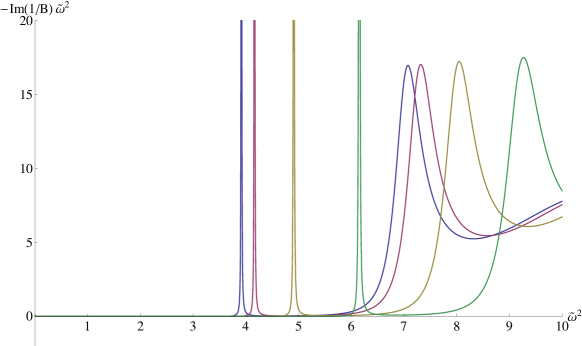
Figure 1: Spectral function of $A_{3}$ for different values of $\tilde{k}$ at $t=0.07$. Blue: $\tilde{k}=0.0$, purple: $\tilde{k}=0.5$, yellow: $\tilde{k}=1.0$, green: $\tilde{k}=1.5$.

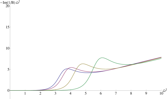
Figure 2: Spectral function of $A_{3}$ for different values of $\tilde{k}$ at $t=0.13$. Blue: $\tilde{k}=0.0$, purple: $\tilde{k}=0.5$, yellow: $\tilde{k}=1.0$, green: $\tilde{k}=1.5$.

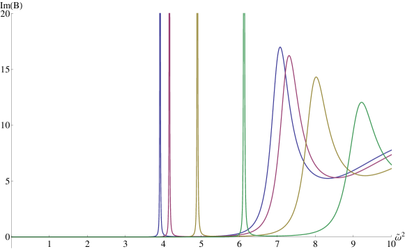
Figure 3: Spectral function of $A_{1}$ for different values of $\tilde{k}$ at $t=0.07$. Blue: $\tilde{k}=0.0$, purple: $\tilde{k}=0.5$, yellow: $\tilde{k}=1.0$, green: $\tilde{k}=1.5$.

Figures 1 and 2 show the melting of the spectral peaks as the temperature is increased. This effect remains the same regardless of the value of $k$. Comparing Figures 1 and 3, it is clear that the spectral functions are not isotropic: if the polarization is tangential to the momentum, the peaks hardly decline; whereas if the polarization is perpendicular to the momentum, the peaks decrease quickly as the momentum is increased. Note that for $k=0$, the spectral functions indeed are the same: this is of course expected as in this case $\mathbf{k}=\mathbf{0}$ and hence full isotropy should be restored indeed.

Figure 1 has the peculiar property that the spectral peaks do not damp as $k$ increases. If one increases $k$ even further, one finds the result of Figure 4.

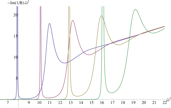
Figure 4: Spectral function of $A_{3}$ for different values of $\tilde{k}$ at $t=0.07$. Blue: $\tilde{k}=2.0$, purple: $\tilde{k}=2.5$, yellow: $\tilde{k}=3.0$, green: $\tilde{k}=3.5$.

IV Influence of magnetic field on the spectral functions

In this section, we will demonstrate how the spectral functions are modified if a background magnetic field $\mathcal{B}$ is turned on. In order to analyze the influence of the magnetic field, we will follow our earlier model Dudal:2014jfa where we proposed a DBI-modification of the soft-wall model to allow the magnetic field to couple to the charged constituents of the mesons. If one compares the differential equations to those described in the previous section, only a few things change. The background $\mathbf{\mathcal{B}}$-field, which we orient along the 3-axis, corresponds to

$$\bar{F}_{12}=-\bar{F}_{21}=\partial_{1}A_{2}=-iq\mathcal{B}\frac{2}{3},$$ (38)

since the charm quark charge is $+2/3q$. We obtain for $\mathcal{G}_{\mu\nu}\equiv g_{\mu\nu}+2\pi\alpha^{\prime}iF_{\mu\nu}$:

$$\mathcal{G}_{\mu\nu}=\left[\begin{array}[]{ccccc}g_{00}&0&0&0&0\\ 0&g_{11}&2\pi\alpha^{\prime}i\bar{F}_{12}&0&0\\ 0&-2\pi\alpha^{\prime}i\bar{F}_{12}&g_{22}&0&0\\ 0&0&0&g_{33}&0\\ 0&0&0&0&g_{zz}\end{array}\right],$$ (44)

with its determinant

$$\mathcal{G}=g_{00}g_{33}g_{zz}\left(g_{11}g_{22}-(2\pi\alpha^{\prime})^{2}\bar{F}_{12}^{2}\right).$$ (45)

We will denote by $G$ only the symmetric part of the metric tensor $\mathcal{G}$:

$$G^{\mu\nu}=\left[\begin{array}[]{ccccc}\frac{1}{g_{00}}&0&0&0&0\\ 0&\frac{g_{22}}{X}&0&0&0\\ 0&0&\frac{g_{11}}{X}&0&0\\ 0&0&0&\frac{1}{g_{33}}&0\\ 0&0&0&0&\frac{1}{g_{zz}}\end{array}\right],$$ (51)

where $X=g_{11}g_{22}-(2\pi\alpha^{\prime})^{2}\bar{F}_{12}^{2}$.

Then substituting these values of $\sqrt{\mathcal{G}}$ and $G^{\mu\nu}$ in the earlier differential equations (21), (22) and (23), one obtains the correct equations for the DBI-modification of the model. Moreover, the asymptotic behavior of the solutions both at the horizon and at the boundary is unaffected by including the magnetic field.

For the sake of brevity, we will only look at the special case where the spatial momentum $\mathbf{k}$ is tangential to the magnetic field $\mathbf{\mathcal{B}}$. The other case can be dealt with analogously but will not be discussed here. The set-up of the different vector quantities is demonstrated in Figure 5.

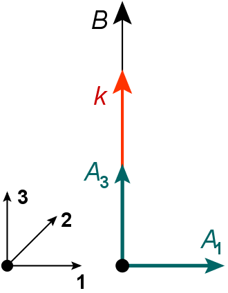
Figure 5: Set-up: the magnetic field is directed along the 3-axis, the momentum is chosen to be tangential to the magnetic field and the two polarizations that we will consider are along the 1- and the 3-axis.

Turning on the magnetic field, one finds the results of Figures 6 and 7.

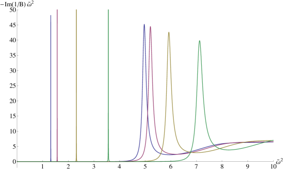
Figure 6: Spectral function of $A_{3}$ with $q\mathcal{B}=1.0$ GeV² for different values of $\tilde{k}$ at $t=0.07$. Blue: $\tilde{k}=0.0$, purple: $\tilde{k}=0.5$, yellow: $\tilde{k}=1.0$, green: $\tilde{k}=1.5$.

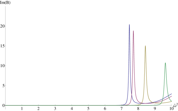
Figure 7: Spectral function of $A_{1}$ with $q\mathcal{B}=1.0$ GeV² for different values of $\tilde{k}$ at $t=0.07$. Blue: $\tilde{k}=0.0$, purple: $\tilde{k}=0.5$, yellow: $\tilde{k}=1.0$, green: $\tilde{k}=1.5$.

First of all, we note that the spectral functions are not the same, even for $k=0$: this corresponds to the breaking of the isotropy already by the magnetic field alone.

Of course, we have only discussed the case where $\mathbf{k}$ and $\mathbf{\mathcal{B}}$ are aligned. The other case where for instance $\mathbf{k}$ is directed along the 1-axis can also be studied analogously, though we will not pursue this here.

Both the results of this and the previous section demonstrate that turning on momentum causes the peaks to shift to higher $\omega$ as expected, where the peak location is at fixed $\omega^{2}-k^{2}$. The reason for this location is that these peaks are identified with the delta-peaks in the thermal AdS case (where $f=1$). In that case, the time direction and the spatial directions along the boundary are fully equivalent (no warping in the $z$-direction) and full Lorentz invariance should be manifestly present.

As a conclusion, all spectral functions widen as $k$ is increased; this implies the excitations melt at a lower temperature in correspondence with Fujita:2009wc ; Fujita:2009ca : the meson melts under the hot wind of the quark-gluon plasma. We do want to remark that the height of the spectral peak on the other hand does not systematically decrease, but this depends on the polarization and the magnitude of the magnetic field.

V Conclusion

We have scrutinized the quite common application of the radiation gauge in holography and demonstrated that for the AdS black hole, one cannot impose this gauge. We then demonstrated that this issue is of physical relevance. This was achieved by showing that the previously observed emergent isotropy for the momentum-dependent (quarkonium) spectral function is actually the result of a faulty choice of gauge. As the momentum $k$ increases, the spectral peaks widen and melt at a lower temperature than before. We furthermore provided some results on the momentum dependence of the spectral functions when including a background magnetic field, following our earlier proposed model Dudal:2014jfa of a DBI-extension of the soft wall model.

References

- (1) J. Erlich, E. Katz, D. T. Son and M. A. Stephanov,“QCD and a holographic model of hadrons,” Phys. Rev. Lett. 95 (2005) 261602 [hep-ph/0501128].
- (2) A. Karch, E. Katz, D. T. Son and M. A. Stephanov, “Linear confinement and AdS/QCD,” Phys. Rev. D 74 (2006) 015005 [hep-ph/0602229].
- (3) A. Karch, E. Katz, D. T. Son and M. A. Stephanov, “On the sign of the dilaton in the soft wall models,” JHEP 1104 (2011) 066 [arXiv:1012.4813 [hep-ph]].
- (4) M. Fujita, K. Fukushima, T. Misumi and M. Murata, “Finite-temperature spectral function of the vector mesons in an AdS/QCD model,” Phys. Rev. D 80 (2009) 035001 [arXiv:0903.2316 [hep-ph]].
- (5) M. Fujita, T. Kikuchi, K. Fukushima, T. Misumi and M. Murata, “Melting Spectral Functions of the Scalar and Vector Mesons in a Holographic QCD Model,” Phys. Rev. D 81 (2010) 065024 [arXiv:0911.2298 [hep-ph]].
- (6) H. R. Grigoryan, P. M. Hohler and M. A. Stephanov, “Towards the Gravity Dual of Quarkonium in the Strongly Coupled QCD Plasma,” Phys. Rev. D 82 (2010) 026005 [arXiv:1003.1138 [hep-ph]].
- (7) L. X. Cui, S. Takeuchi and Y. L. Wu, “Thermal Mass Spectra of Vector and Axial-Vector Mesons in Predictive Soft-Wall AdS/QCD Model,” JHEP 1204 (2012) 144 [arXiv:1112.5923 [hep-ph]].
- (8) S. He, S. Y. Wu, Y. Yang and P. H. Yuan, “Phase Structure in a Dynamical Soft-Wall Holographic QCD Model,” JHEP 1304 (2013) 093 [arXiv:1301.0385 [hep-th]].
- (9) P. M. Hohler and Y. Yin,“Charmonium moving through a strongly coupled QCD plasma: a holographic perspective,” Phys. Rev. D 88 (2013) 086001 [arXiv:1305.1923 [nucl-th]].
- (10) Y. Yang and P. H. Yuan, “Confinement-Deconfinement Phase Transition for Heavy Quarks,” arXiv:1506.05930 [hep-th].
- (11) K. Peeters, J. Sonnenschein and M. Zamaklar, “Holographic melting and related properties of mesons in a quark gluon plasma,” Phys. Rev. D 74 (2006) 106008 [hep-th/0606195].
- (12) T. Ishii, S. Kinoshita, K. Murata and N. Tanahashi, “Dynamical Meson Melting in Holography,” JHEP 1404 (2014) 099 [arXiv:1401.5106 [hep-th]].
- (13) M. Ali-Akbari, Z. Rezaei and A. Vahedi, “Thermal Fluctuation and Meson Melting: Holographic Approach,” J. Phys. G 42 (2015) 7, 075001 [arXiv:1406.2900 [hep-th]].
- (14) S. Hong, S. Yoon and M. J. Strassler, “Quarkonium from the fifth-dimension,” JHEP 0404 (2004) 046 [hep-th/0312071].
- (15) Y. Kim, J. P. Lee and S. H. Lee,“Heavy quarkonium in a holographic QCD model,” Phys. Rev. D 75 (2007) 114008 [hep-ph/0703172].
- (16) D. Hou and H. c. Ren, Heavy Quarkonium States with the Holographic Potential,” JHEP 0801 (2008) 029 [arXiv:0710.2639 [hep-ph]].
- (17) Y. Hatta, E. Iancu and A. H. Mueller, “Jet evolution in the N=4 SYM plasma at strong coupling,” JHEP 0805 (2008) 037 [arXiv:0803.2481 [hep-th]].
- (18) D. Dudal and T. G. Mertens, “Melting of charmonium in a magnetic field from an effective AdS/QCD model,” Phys. Rev. D 91 (2015) 086002 [arXiv:1410.3297 [hep-th]].
- (19) D. T. Son and A. O. Starinets, “Minkowski space correlators in AdS/CFT correspondence: Recipe and applications,” JHEP 0209 (2002) 042 [hep-th/0205051].
- (20) G. Policastro, D. T. Son and A. O. Starinets, “From AdS/CFT correspondence to hydrodynamics,” JHEP 0209 (2002) 043 [hep-th/0205052].
- (21) D. Teaney, “Finite temperature spectral densities of momentum and R-charge correlators in N=4 Yang Mills theory,” Phys. Rev. D 74 (2006) 045025 [hep-ph/0602044].
- (22) K. Skenderis and B. C. van Rees, “Real-time gauge/gravity duality,” Phys. Rev. Lett. 101 (2008) 081601 [arXiv:0805.0150 [hep-th]].
- (23) K. Skenderis and B. C. van Rees, “Real-time gauge/gravity duality: Prescription, Renormalization and Examples,” JHEP 0905 (2009) 085 [arXiv:0812.2909 [hep-th]].
- (24) J. Lindgren, I. Papadimitriou, A. Taliotis and J. Vanhoof, “Holographic Hall conductivities from dyonic backgrounds,” JHEP 1507 (2015) 094 [arXiv:1505.04131 [hep-th]].