The turbulent destruction of clouds - III. Three dimensional adiabatic shock-cloud simulations

Abstract

We present 3D hydrodynamic simulations of the adiabatic interaction of a shock with a dense, spherical cloud. We compare how the nature of the interaction changes with the Mach number of the shock, $M$, and the density contrast of the cloud, $\chi$. We examine the differences with 2D axisymmetric calculations, perform detailed resolution tests, and compare “inviscid” results to those obtained with the inclusion of a $k$-$\epsilon$ subgrid turbulence model. Resolutions of 32-64 cells per cloud radius are the minimum necessary to capture the dominant dynamical processes in 3D simulations, while the 3D inviscid and $k$-$\epsilon$ simulations typically show very good agreement. Clouds accelerate and mix up to 5 times faster when they are poorly resolved. The interaction proceeds very similarly in 2D and 3D - although non-azimuthal modes lead to different behaviour, there is very little effect on key global quantities such as the lifetime of the cloud and its acceleration. In particular, we do not find significant differences in the hollowing or “voiding” of the cloud between 2D and 3D simulations with $M=10$ and $\chi=10$, which contradicts previous work in the literature.

1 Introduction

The interaction of fast, rarefied gas with denser “clouds” is a common occurence in astrophysics and much effort has been invested to understand this process. Clouds struck by shocks or winds can be destroyed, “mass-loading” the flow and affecting its nature. Such interactions have implications for our understanding of the nature of the interstellar medium (ISM; see, e.g., Elmegreen & Scalo, 2004; Scalo & Elmegreen, 2004), for the evolution of diffuse sources such as supernova remnants (McKee & Ostriker, 1977; Chièze & Lazareff, 1981; Cowie et al., 1981; White & Long, 1991; Arthur & Henney, 1996; Dyson et al., 2002; Pittard et al., 2003), and for galaxy formation and evolution (e.g., Sales et al., 2010).

Shock-cloud interactions in supernova remnants (SNRs) are some of the best observed and studied cases to date. Some SNRs display large-scale distortions which are associated with their interaction with nearby molecular clouds (see, e.g., a recent review by Slane et al., 2015). Examples include the Cygnus Loop (Graham et al., 1995; Levenson et al., 1999), Tycho (Katsuda et al., 2010; Williams et al., 2013), and SN 1006 (Miceli et al., 2014; Winkler et al., 2014). SNR-cloud interactions are also revealed by the presence of OH (1720 MHz) masers (e.g., Brogan et al., 2013), an enhanced ¹²CO($J=2-1$)/¹²CO($J=1-0$) ratio in the line wings (Seta et al., 1998), and temperature, absorption and ionization variations in X-ray emission (e.g., Chen & Slane, 2001; Koo et al., 2005; Nakamura et al., 2014). SNR-cloud interactions are often radiative, and produce optical, IR and sub-mm line emission (e.g., as seen in IC 433; Fesen & Kirshner, 1980; Snell et al., 2005; Bykov et al., 2008; Kokusho et al., 2013). $\gamma$-ray emission, which to date has been detected from about 25 SNRs (Slane et al., 2015), may also arise when SNRs interact with molecular clouds. In two cases, W44 and IC 433, this emission is established to be from energetic ions, and so is unambiguously from the SNR shock (Abdo et al., 2010; Giuliani et al., 2011; Ackermann et al., 2013). A list of galactic SNRs thought to be interacting with surrounding clouds is given in the appendix of Jiang et al. (2010).

In other SNRs much finer features indicate interaction with much smaller clouds, either in the ISM or in the ejecta. Significant observational evidence now exists for clumpy ejecta, especially in core-collapse SNe (e.g., Filippenko & Sargent, 1989; Spyromilio, 1991, 1994; Fassia et al., 1998; Matheson et al., 2000; Elmhamdi et al., 2004). The best observed examples of ejecta clumps are those seen in the Vela remnant (Aschenbach et al., 1995; Strom et al., 1995; Tsunemi et al., 1999; Katsuda & Tsunemi, 2006) and in Cassiopeia A (Cas A) (e.g., Kamper & van den Bergh, 1976; Chevalier & Kirshner, 1979; Reed et al., 1995; Fesen, 2001; Fesen et al., 2011; Milisavljevic & Fesen, 2013; Patnaude & Fesen, 2014; Alarie et al., 2014). N132D (Lasker, 1978, 1980; Morse et al., 1996; Blair et al., 2000), Puppis A (Winkler & Kirshner, 1985; Katsuda et al., 2008), SNR G292.0+1.8 (Park et al., 2004; Ghavamian et al., 2005) and the SMC SNR 1E 0102-7219 (Finkelstein et al., 2006) also display ejecta bullets.

In Cas A ejecta knots are seen both ahead of the main forward shock, where they interact with the circumstellar or interstellar medium, and just after their passage through the remnant’s reverse shock. Some of the outer ejecta knots in Cas A show emission trails indicative of mass ablation, which Fesen et al. (2011) argue form best if the cloud density contrast $\chi=10^{3}$ (clouds with $\chi=10^{2}$ are destroyed too rapidly, while too little material is ablated when $\chi=10^{4}$). Patnaude & Fesen (2014) instead present evidence for mass-ablation from the inner ejecta knots in Cas A. Enhanced X-ray emission which extends $1-2\arcsec$ downstream of the shocked clumps is interpreted as stripped material which is heated to X-ray emitting temperatures in the tail. For knot sizes of $a_{\rm 0}\sim 10^{15}-10^{16}\,$cm, this equates to $5-100\,a_{\rm 0}$, and is compatible with the tail lengths found in Pittard et al. (2010) A number of other studies have considered the ejecta clumps in Vela, with the particular goal of reproducing the protrusions ahead of the blast shock. Wang & Chevalier (2002) found that the survival of the ejecta clumps through the reverse shock and out past the forward shock required an initial $\chi\sim 10^{3}$. Miceli et al. (2013) find that lower values of $\chi$ are acceptable if the effects of radiative cooling and thermal conduction are included.

The middle-aged ($\sim 3700\,$yr; Winkler et al., 1988) SNR Puppis A is interacting with several interstellar clouds, of which the most prominent is known as the bright eastern knot. Hwang et al. (2005) present a Chandra observation of this region, and identify two main morphological components. The first is a bright compact knot that lies directly behind an indentation in the main shock front. The second component lies about $1\arcsec$ downstream of the shock and consists of a curved vertical structure (the “bar”) separated from a smaller bright cloud (the “cap”) by faint diffuse emission. Based on hardness images and spectra, and comparing to the “voided sphere” structures seen by Klein et al. (2003), the bar and cap structure is identified as a single shocked interstellar cloud. The interaction is inferred to have $\chi=10$, and to be at a relatively late stage of evolution ($t\sim 3\,t_{\rm cc}$, where $t_{\rm cc}$ is the characteristic cloud crushing timescale - see Sec. 3). The compact knot directly behind the shock front is identified as a more recent interaction with another cloud. Another well-studied interaction between a SNR and a small ($<1\,$pc) interstellar cloud is FilD in the Vela SNR. Miceli et al. (2006) estimate that a Mach 57 shock is in the early stages of interacting with an ellipsoidal cloud with $\chi=30$.

Numerical studies of shock-cloud interactions have now been performed for many decades. However, the motivation for the current work comes from our realization that, barring the work in the code development paper of Schneider & Robertson (2015), all 3D “pure-hydrodynamic” shock-cloud calculations (i.e. those without additional physical processes such as cooling, magnetic fields, thermal conduction and gravity) in the astrophysics literature are for one set of parameters only: $M=10$ and $\chi=10$ (see Sec. 2.1 and Table 1). We therefore extend the 2D work in Pittard et al. (2009, 2010) to 3D. The extension to 3D is necessary for two reasons: i) non-axisymmetric perturbations can only be obtained in 3D; ii) the late-time flow in shock-cloud interactions can acquire characteristics similar to turbulence, which has a fundamentally different behaviour in 2D due to the absence of vortex-stretching (in 2D, vortices are well-defined and long-lasting).

We investigate 3D shock-cloud interactions for Mach numbers $M=1.5,\,3$ and 10, and for density contrasts $\chi=10,\,10^{2}$, and $10^{3}$. This extends the $\chi$ parameter space to $10\times$ higher values than any previously published 3D simulation that we are aware, and a factor of 25 higher than any previously published 3D adiabatic simulation. As in our previous 2D work we present “inviscid” simulations and simulations with a $k$-$\epsilon$ subgrid turbulence model. In Sec. 2 we review the numerical and experimental work which currently exists. In Sec. 3 we describe the simulation setup and in Sec. 4 we present our results. As well as describing the 3D nature of the interaction, we compare our 3D results to those from 2D simulations. In Sec. 5 we summarize our results and draw conclusions. A detailed resolution test is presented in an appendix. In a follow-up paper (Pittard & Goldsmith, 2016), an investigation of a shock striking a filament (as opposed to a spherical cloud) will be presented.

2 The interaction of a shock with a cloud

2.1 Numerical studies

The idealized problem of the hydrodynamical interaction of a planar adiabatic shock with a single isolated cloud was first studied numerically in the 1970s. The evolution of the cloud can be described in terms of a characteristic cloud-crushing timescale, and is scale-free for strong shocks. The cloud is first compressed, becomes overpressured, and then re-expands, and is subject to a variety of dynamical instabilities, including Kelvin-Helmholtz (KH), Rayleigh-Taylor (RT) and Richtmyer-Meshkov (RM). Strong vorticity is deposited at the surface of the cloud and this vorticity aids in the subsequent mixing of cloud and ambient material. Detailed two-dimensional (2D) axisymmetric calculations by Klein, McKee & Colella (1994) showed that a numerical resolution of about 120 cells per cloud radius (hereafter referred to as $R_{120}$) was required in order to properly capture the main features of the interaction. The effects of smooth cloud boundaries, radiative cooling, thermal conduction and magnetic fields have now been considered (see Pittard et al., 2010, for a summary of work up until 2010). The interaction is milder at lower shock Mach numbers (see, e.g., Nakamura et al., 2006), and when the post-shock gas is subsonic with respect to the cloud a bow-wave instead of a bow-shock forms.

A dedicated study of how the adiabatic interaction of a shock with a cloud depends on $M$, $\chi$ and the numerical resolution was recently presented by Pittard et al. (2009, 2010). Using 2D axisymmetric simulations, the results from “inviscid” models with no explicit artificial viscosity were compared against results when a $k$-$\epsilon$ subgrid turbulence model is included. The 2D inviscid models confirmed that a resolution of approximately $R_{100}$ is necessary for convergence in simple adiabatic simulations. However, this requirement was found to reduce to $\sim R_{32}$ when a subgrid turbulence model is included. The cloud lifetime, defined as the point when material from the core of the cloud is well mixed with the ambient material, is about $t_{\rm mix}\sim 6\,t_{\rm KHD}$, where $t_{\rm KHD}$ is the growth-timescale for the most disruptive, long-wavelength, KH instabilities. Cloud density contrasts $\chi\mathrel{\hbox to0.0pt{\lower 3.0pt\hbox{$\sim$}\hss}\raise 2.0pt\hbox{$>$}}10^{3}$ are required for the cloud to form a long tail-like feature.

The first three-dimensional (3D) shock-cloud calculation was presented by Stone & Norman (1992). The simulation was adiabatic, had $M=10$ and $\chi=10$, and used a numerical resolution of $R_{60}$. More rapid mixing was observed since 3D hydrodynamical instabilities are able to fragment the cloud in all directions, although this was not quantified. Subsequently, Klein et al. (2003) noted that 2D hydrodynamical simulations did not compare well against experimental results obtained with the Nova laser, which showed a “voiding” of the shocked cloud, and break up of the vortex ring by the azimuthal bending-mode instability (Widnall et al., 1974). Crucially, a 3D simulation reproduced both of these features. Other 3D work in the astrophysics literature (summarized in Table 1) has investigated the effects of additional physics, including the cloud shape and edges, radiative cooling, thermal conduction and magnetic fields (Xu & Stone, 1995; Orlando et al., 2005; Nakamura et al., 2006; Shin, Stone & Snyder, 2008; Van Loo, Falle & Hartquist, 2010; Johansson & Ziegler, 2013; Vaidya, Hartquist & Falle, 2013; Li, Frank & Blackman, 2013; Schneider & Robertson, 2015).

Additional 3D simulations have been used to study the behaviour of clouds accelerated by winds (e.g., Gregori et al., 2000; Agertz et al., 2007; Raga et al., 2007; Kwak et al., 2011; McCourt et al., 2015; Scannapieco & Brüggen, 2015), by finite-thickness supernova blast waves (e.g., Leaõ et al., 2009; Obergaulinger et al., 2014), or by dense shells (Pittard, 2011). The ram-pressure stripping of the interstellar medium from galaxies (e.g., Close et al., 2013; Shin & Ruszkowski, 2013, 2014; Tonnesen & Stone, 2014; Roediger et al., 2015a, b; Vijayaraghavan & Ricker, 2015) has also been considered. Though each of these scenarios are similar in some ways to a shock-cloud interaction, the details differ in each case, and therefore we do not discuss these works further.

Outside of the astrophysics literature, the shock-cloud interaction is commonly referred to as a shock-bubble interaction (the bubble can be lighter or denser than the surrounding medium). Simulations carried out by the fluid dynamics community have focused on a similar region of parameter space as their experiments, which for practical reasons tend to have lower $\chi$ and $M$ than the work noted in Table 1. In the most comprehensive 3D study to date (performed at a resolution of $R_{128}$), Niederhaus et al. (2008) examined shock Mach numbers up to 5, and cloud density contrasts up to 4.2. They also considered different (fixed) values of the ratio of specific heats, $\gamma$, for the ambient and cloud gas. The work by Niederhaus et al. (2008) is also noteable for its detailed study into the development and behaviour of vorticity. In a 2D axisymmetric simulation, the vorticity can only have a $\theta$-component, and the late-time flow is dominated by large and distinct vortex rings. However, in 3D simulations, this restriction no-longer applies, and the vorticity develops components in the axial and radial directions. Niederhaus et al. (2008) find that when $\chi\mathrel{\hbox to0.0pt{\lower 3.0pt\hbox{$\sim$}\hss}\raise 2.0pt\hbox{$>$}}1.5$, the axial and radial components of the vorticity grow to a similar magnitude as the azimuthal component - it is this growth which accounts for the differences in the late-time flow-field in 2D and 3D simulations. Niederhaus et al. (2008) also find that the degree of mixing of cloud and ambient material increases as $\chi$ increases, due to the greatly increased complexity and intensity of scattered shocks and rarefaction waves, which ultimately cause the formation of the turbulent wake.

Finally, we note that Ranjan et al. (2008) present 3D hydrodynamical simulations of a Mach 5 interaction of an R12 bubble in air ($\chi=4.17$) with a resolution of $R_{134}$. They find that the vorticity field becomes so complex that the primary vortex core becomes almost indistinguishable.

2.2 Shock-cloud laboratory experiments

There are two broad types of laboratory experiments: those which use a conventional shock-tube, and those which are laser-driven. The literature has recently been reviewed by Ranjan et al. (2011). Of most relevance to this work are the shock-bubble experiments of Layes et al. (2009), who reported shock waves ($M=1.05$, 1.16, 1.4 and 1.61) through air striking a krypton gas bubble ($\chi=2.93$), the experimental results of Ranjan et al. (2008) for $M=2.05$ and 3.38 shocks striking an argon bubble in nitrogen ($\chi=1.43$), an $M=2.03$ shock striking a bubble of R22 refrigerant gas ($\chi=3.13$), and $M=2.07$ and 3.0 shocks striking a sulfur-hexafluoride bubble ($\chi=5.27$), and the experiments of Zhai et al. (2011) of a sulfur-hexafluoride bubble in air, with $M=1.23$ and $\chi=5.04$. Also noteable are the experiments by Ranjan et al. (2005) of an argon bubble in nitrogen struck by an $M=2.88$ shock, which provided the first detection of distinct secondary vortex rings.

Laser-driven experiments of strong shocks ($M\approx 10$) interacting with a copper, aluminium or sapphire sphere embedded in a low-density plastic or foam ($\chi\approx 8-10$) have been reported by Robey et al. (2002), Hansen et al. (2007) and Rosen et al. (2009) for the Omega laser at the Laboratory of Laser Energetics, and by Klein et al. (2000, 2003) for the Nova laser at the Lawrence Livermore National Laboratory. In particular, Klein et al. (2000) found the first evidence of 3D bending mode instabilities in high Mach number shock-cloud interactions. The experimental results also indicate much faster destruction and mixing of the cloud at late times than occurs in 2D simulations (see Figs. 12 and 13 in Klein et al., 2003). Robey et al. (2002) detect a double vortex ring structure with a dominant azimuthal mode number of $\approx 5$ for the inner ring, and $\approx 15$ for the outer ring. 3D numerical simulations are found to be in very good agreement. Hansen et al. (2007) are able to estimate the mass of the cloud as a function of time. They find that a laminar model overestimates the stripping time by an order of magnitude, and conclude that the mass-stripping must be turbulent in nature. Rosen et al. (2009) find that their 3D simulations broadly agree with the gross features in their experimental data, but differ in the finer-scale structure.

Table 1: A summary of previous 3D numerical investigations of shock-cloud interactions in the astrophysics literature. $\chi$ is the density contrast of the cloud with respect to the ambient medium and $M$ is the shock Mach number. The references are as follows: ^aStone & Norman (1992); ^bXu & Stone (1995); ^cKlein et al. (2000, 2003); ^dOrlando et al. (2005); ^eNakamura et al. (2006); ^fShin et al. (2008); ^gVan Loo et al. (2010); ^hJohansson & Ziegler (2013); ⁱVaidya et al. (2013); ^jLi et al. (2013); ^kSchneider & Robertson (2015).

Authors	Typical (max)	$\chi$	$M$	Cooling?	Conduction?	Magnetic
	resolution					fields?
SN92a	60 (60)	10	10
XS95b	25 (53)	10	10
K00/03c	90	10	10
O05d	132 (132)	10	30,50	✔	✔
N06e	60	10	10
SSS08f	68 (68)	10	10			✔
VL10g	120	45	2.5	✔		✔
JZ13h	100	100	30	✔	anisotropic	✔
V13i	225+	17.8	1.5,2	isothermal		✔
L13j	54	100	10	✔		✔
SR15k	54	10,20,40	50

3 The Numerical Setup

Our calculations were performed on a 3D XYZ cartesian grid using the MG adaptive mesh refinement (AMR) hydrodynamic code. MG uses piece-wise linear cell interpolation to solve the Eulerian equations of hydrodynamics. The Riemann problem is solved at cell interfaces to obtain the conserved fluxes for the time update. A linear Riemann solver is used for most cases, with the code switching to an exact solver when there is a large difference between the two states (Falle, 1991). Refinement is performed on a cell-by-cell basis and is controlled by the difference in the solutions on the coarser grids. The flux update occurs for all directions simultaneously. The time integration proceeds first with a half time-step to obtain fluxes at this point. The conserved variables are then updated over the full time-step. The code is 2^nd-order accurate in space and time. The full set of equations solved (including when the subgrid turbulence model is employed) is given in Pittard et al. (2009). We limit ourselves to a purely hydrodynamic study in this work, and ignore the effects of magnetic fields, thermal conduction, cooling and self-gravity. All calculations were perfomed for an ideal gas with $\gamma=5/3$ and are adiabatic. Our calculations are thus scale-free and can be easily converted to any desired physical scales.

The cloud is initially in pressure equilibrium with its surroundings and is assumed to have soft edges (typically over about 10 per cent of its radius). The equation for the cloud profile is noted in Pittard et al. (2009) - in keeping with the results from this earlier work we again adopt $p_{1}=10$ (i.e. a reasonably hard-edged cloud). An advected scalar is used to distinguish between cloud and ambient material, and can be used to track the ablation and mixing of the cloud, and the cloud’s acceleration by the passage of the shock and subsequent exposure to the post-shock flow.

The cloud is initially centered at the grid origin $(x,y,z)=(0,0,0)$. The grid has zero gradient conditions on each boundary and is set large enough so that the cloud is well-dispersed and mixed into the post-shock flow before the shock reaches the downstream boundary. The grid extent is dependent on $\chi$ (clouds with larger density contrasts take longer to be destroyed) and is noted in Table 2. Our grid extent is often significantly greater than previously adopted in the literature. Note that we also do not impose any symmetry constraints on the interaction (unlike some of the 3D work in the literature, e.g., Stone & Norman, 1992; Xu & Stone, 1995; Orlando et al., 2005; Niederhaus et al., 2008), and thus all quadrants are calculated. The simulations are generally evolved until $t\sim 20\,t_{\rm cc}$, though at lower Mach numbers they are run to $t\sim 80\,t_{\rm cc}$.

We also perform new 2D axisymmetric calculations at $R_{128}$ resolution and with a similar grid extent. To compare our 3D simulations against these, we define motion in the direction of shock propagation as “axial” (the shock propagates along the X-axis), and refer to it with a subscript “z”, while we collapse the Y and Z directions to obtain a “radial”, or “r” coordinate.

Table 2: The grid extent for the 3D simulations, which depends on the shock Mach number, $M$, and the cloud density contrast, $\chi$. The unit of length is the cloud radius, $r_{\rm c}$.

$M$	$\chi$	X	Y,Z
10	10	$-5<X<65$	$-10<Y,Z<10$
	$10^{2}$	$-5<X<95$	$-16<Y,Z<16$
	$10^{3}$	$-5<X<475$	$-24<Y,Z<24$
3	10	$-6<X<154$	$-16<Y,Z<16$
	$10^{2}$	$-6<X<474$	$-16<Y,Z<16$
	$10^{3}$	$-6<X<474$	$-16<Y,Z<16$
1.5	10	$-150<X<300$	$-20<Y,Z<20$
	$10^{2}$	$-200<X<600$	$-20<Y,Z<20$
	$10^{3}$	$-290<X<910$	$-20<Y,Z<20$

Table 3: The maximum resolution $N$ (defined as the number of cells per could radius) used as a function of $M$ and $\chi$.

$\chi$/M	1.5	3	10
10	64	64	128
$10^{2}$	32	64	128
$10^{3}$	32	64	64

Various integrated quantities are monitored to study the evolution of the interaction (see Klein et al., 1994; Nakamura et al., 2006; Pittard et al., 2009). Averaged quantities $\langle f\rangle$, are constructed by

$$\langle f\rangle=\frac{1}{m_{\beta}}\int_{\kappa\geq\beta}\kappa\rho f\;dV,$$ (1)

where the mass identified as being part of the cloud is

$$m_{\beta}=\int_{\kappa\geq\beta}\kappa\rho\;dV.$$ (2)

$\kappa$ is an advected scalar, which has an initial value of $\rho/(\chi\rho_{\rm amb})$ for cells within a distance of $2r_{\rm c}$ from the centre of the cloud, and a value of zero at greater distances. Hence, $\kappa=1$ in the centre of the cloud, and declines outwards. The above integrations are performed only over cells in which $\kappa$ is at least as great as the threshold value, $\beta$. Setting $\beta=0.5$ probes only the densest parts of the cloud and its fragments (identified with the subscript “core”), while setting $\beta=2/\chi$ probes the whole cloud including its low density envelope, and regions where only a small percentage of cloud material is mixed into the ambient medium (identified with the subscript “cloud”).

The integrated quantities which are monitored in the calculations include the effective radii of the cloud in the radial ($a$) and axial ($c$) directions. These are defined as

$$a=\left(\frac{5}{2}\langle r^{2}\rangle\right)^{1/2},\;\;\;\;\;\;c=\left[5\left(\langle z^{2}\rangle-\langle z\rangle^{2}\right)\right]^{1/2},$$ (3)

where we convert our 3D XYZ coordinate system into a 2D rz coordinate system through $r=\sqrt{(}Y^{2}+Z^{2})$ and $z=X$.

We also monitor the velocity dispersions in the radial and axial directions, defined respectively as

$$\delta v_{\rm r}=\left<v_{\rm r}^{2}\right>^{1/2},\;\;\;\;\;\delta v_{\rm z}=\left(\left<v_{\rm z}^{2}\right>-\langle v_{\rm z}\rangle^{2}\right)^{1/2},$$ (4)

the cloud mass ($m$), and its mean velocity in the axial direction ($\langle v_{\rm z}\rangle$, measured in the frame of the unshocked cloud). The whole of the cloud and the densest part of its core are distinguished by the value of the scalar variable $\kappa$ associated with the cloud (see Pittard et al., 2009). In this way, each global statistic can be computed for the region associated only with the core (e.g., $a_{\rm core}$) or with the entire cloud (e.g., $a_{\rm cloud}$).

The characteristic time for the cloud to be crushed by the shocks driven into it is the “cloud crushing” time, $t_{\rm cc}=\chi^{1/2}r_{\rm c}/v_{\rm b}$, where $v_{\rm b}$ is the velocity of the shock in the intercloud (ambient) medium (Klein et al., 1994). Several other timescales are obtained from the simulations. The time for the average velocity of the cloud relative to that of the postshock ambient flow to decrease by a factor of 1/$e$ is defined as the “drag time”, $t_{\rm drag}$. The “mixing time”, $t_{\rm mix}$, is defined as the time when the mass of the core of the cloud, $m_{\rm core}$, reaches half of its initial value. The “life time”, $t_{\rm life}$, is defined as the time when $m_{\rm core}=0$. The zero-point of all time measurements occurs when the intercloud shock is level with the centre of the cloud.

An effective or grid-scale Reynolds number can be derived for our inviscid simulations. The largest eddies have a length scale, $l$, which is comparable to the size of the cloud ($l\sim 2r_{\rm c}$), while the minimum eddy size, $\eta\approx 2\Delta x$, where $\Delta x$ is the cell size. Since the Reynolds number, $Re=(l/\eta)^{4/3}$, we find that $Re\sim 650$ in our $R_{128}$ 3D simulations. The effective Reynolds number is likely to be $\mathrel{\hbox to0.0pt{\lower 3.0pt\hbox{$\sim$}\hss}\raise 2.0pt\hbox{$>$}}10^{3}$ in the tail region of some simulations, where the tail is several times broader than the original cloud.

4 Results

We begin by examining the level of convergence in our simulations: i.e. that the calculations are performed at spatial resolutions that are high enough to resolve the key features of the interaction. Increasing the resolution in inviscid calculations leads to smaller scales of instabilities. Quantities which are sensitive to these small scales (such as the mixing rate between cloud and ambient gas) may not be converged, while quantities which are insensitive to gas motions at small scales (e.g., the shape of the cloud) are more likely to show convergence. Previous 2D studies (e.g., Klein et al., 1994; Nakamura et al., 2006) have indicated that about 100 cells per cloud radius are needed for convergence of the simulations. Pittard et al. (2009) demonstrated that $k$-$\epsilon$ simulations converged at lower resolution.

In Appendix A we carry out a similar study for 3D calculations with and without the use of a subgrid turbulence model. Appendix A.1 shows that resolutions of at least $R_{64}$ are necessary to properly capture the nature of the interaction in terms of the appearance and morphology of the cloud. However, Appendix A.2 and A.3 show that the broad evolution of the cloud can often be adequately captured at lower resolution, for instance at $R_{32}$. This is helpful considering the much greater computational demands of 3D simulations. Another key finding is that 3D inviscid and $k$-$\epsilon$ models are often in very good agreement. Comparing the morphology, we typically find that the core structure is almost identical (being dominated by shocks and rarefaction waves) until later times. Instead, the $k$-$\epsilon$ model tends to reveal its presence in the cloud tail and wake, where it tends to smooth out the flow (this region is dominated by eddies and vortices). This is a surprising result given that 2D calculations can show significant differences (see Pittard et al., 2009, 2010), but must be related to the different way that vortices behave and evolve in 2D and 3D flows. Since we find no compelling benefit from using the $k$-$\epsilon$ model in 3D calculations, in the rest of this work our focus will therefore be on the inviscid simulations.

Figure 1: A 3D volumetric rendering of the time evolution of the $M=10$, $\chi=10$ simulation. From left to right and top to bottom the times are $t=0.65,1.08,1.94$ and $4.09\,t_{\rm cc}$ ($t=0$ is defined as the time when the intercloud shock is level with the centre of the cloud). The colour indicates the density of the cloud material, normalized by the ambient density (i.e. the initial cloud density is 10). Since the ambient material is not shown the bowshock upstream of the cloud is not visible. The actual grid extends much further than the bounding box shown.

Figure 2: 2D versus 3D comparison of the time evolution of the $M=10$, $\chi=10$ simulation. In each frame, 2D axisymmetric results are shown on the left, and part of the $+Y$, $Z=0$ plane from the 3D simulation is shown on the right. The grayscale shows the logarithm of the mass density, from $\rho_{\rm amb}$ (white) to $5\rho_{\rm c}$ (black). Each frame is labelled with the time, and extends $3\,r_{\rm c}$ off-axis. The first 4 frames show the same region ($-2<X<4$, in units of $r_{\rm c}$) so that the motion of the cloud is clear. The displayed region is shifted in the other frames in order to show the cloud. The frames at $t=3.66$ and $4.52\,t_{\rm cc}$ show $2<X<8$, while the remaining frames show $5<X<11$, $6<X<12$, $8<X<14$ and $9.5<X<15.5$ at $t=5.37$, 6.23, 7.09 and $7.95\,t_{\rm cc}$, respectively. Note that in this and similar figures the $X$-axis is plotted vertically, with positive down.

Figure 3: A 3D volumetric rendering of the time evolution of the $M=10$, $\chi=10$ hard-edged-cloud simulation. Left: $t=1.94\,t_{\rm cc}$. Right: $t=4.09\,t_{\rm cc}$. Other details are as in Fig. 1.

Figure 4: 2D versus 3D comparison of the time evolution of the $M=10$, $\chi=10$, hard-edged-cloud simulation. All details are as Fig. 2.

Figure 5: Comparison of the time evolution of the $M=10$, $\chi=10$, 3D simulations for hard-edged clouds (left “HE” plot in each panel) and soft-edged clouds (right “SE” plot in each panel). All other details are as in Fig. 2.

Figure 6: As Fig. 1 but for $M=10$ and $\chi=10^{2}$. The panels are at $t=0.48,1.16,1.84$ and $3.87\,t_{\rm cc}$. The initial cloud density is 100.

Figure 7: As Fig. 2 but for $M=10$ and $\chi=10^{2}$. Each frame extends $4\,r_{\rm c}$ off-axis. The first 3 frames show the same region ($-2<X<6$, in units of $r_{\rm c}$) so that the motion of the cloud is clear. The final frame shows $4<X<12$.

Figure 8: As Fig. 1 but for $M=10$ and $\chi=10^{3}$. The panels are at $t=0.58,0.80,1.65$ and $3.80\,t_{\rm cc}$. The initial cloud density is $10^{3}$.

Figure 9: As Fig. 2 but for $M=10$ and $\chi=10^{3}$. The first 3 frames show the same region ($-2<X<6$, $0<Y<4$ in units of $r_{\rm c}$) so that the motion of the cloud is clear. The final frame shows $2<X<20$, $0<Y<9$. Note that the 2D simulation has a resolution of $R_{128}$, while the 3D simulation is at the lower resolution of $R_{64}$.

4.1 Cloud Morphology

4.1.1 The interaction of an $M=10$ shock with a $\chi=10$ cloud

We begin by examining the time evolution of the cloud material in the 3D $M=10$, $\chi=10$ simulation (Fig. 1). The bowshock and other features in the ambient medium are not visible in this plot due to this focus. The blue “block” of material advected rapidly downstream represents some “trace” material which highlights roughly where the main shock is. It is added only for visualisation purposes to Figs. 1, 10 and 25.

In the initial stages of the interaction, the transmitted shock front becomes strongly concave and undergoes shock focusing, with the cloud acting like a strongly convergent lens, refracting the transmitted shock towards the axis (see also Fig. 2). Meanwhile the external shock diffracts around the cloud, remaining nearly normal to the cloud surface as it sweeps from the equator to the downstream pole. A dramatic pressure jump occurs as it is focused onto the axis, and secondary shocks are driven into the back of the cloud. Shortly after, the transmitted shock moving through the cloud reaches the back of the cloud. It then accelerates downstream into the lower density ambient gas, and a rarefaction wave is formed which moves back towards the front of the cloud. The secondary shocks deposit further baryoclinic vorticity as they pass through the cloud, and together with the reflected rarefaction waves cause the cloud to reverberate. Shocks leaving the cloud introduce reflected rarefaction waves into the cloud, while diffraction and focusing processes introduce additional shocks into the cloud. Rarefaction waves within the cloud which reach the cloud boundary introduce a transmitted rarefaction wave into the external medium and a reflected shock which moves back into the cloud.

At this point, the centre of the cloud becomes hollow for a moment (see the panel at $t=1.94\,t_{\rm cc}$ in Fig. 2), before the upstream and downstream surfaces collide together and the cloud attains an “arc-like” morphology (see the panel at $t=2.80\,t_{\rm cc}$ in Fig. 2). Some lateral expansion of the cloud has occurred as a result of the lower pressure which exists at the sides of the cloud. The strong shear across the surface of the arc-like cloud also causes instabilities to grow and results in material being stripped off. The cloud then deforms, resulting in a ring of material being ripped off the rest of the cloud. The final panel in Fig. 1 shows this occuring.

The misalignment of the local pressure and density gradients results in the generation of vorticity in the flow field. The maximum misalignment occurs at the sides of the cloud, and this is where the maximum vorticity is deposited. The vortex sheet deposited on the surface of the cloud rolls up into a torus to form a vortex ring. This torus later disintegrates into many vortex filaments under the action of hydrodynamic instabilities.

The features seen in Fig. 1 bear some resemblance to those in Fig. 1 of Stone & Norman (1992) and in Fig. 2 of Xu & Stone (1995), but it is clear that there are some differences. In both works the initial shock position is at $x=-1.2$ (this is true in Xu & Stone’s work for their high resolution simulation), so the elapsed time before the shock is level with the centre of the cloud is $\approx 0.09\,t_{\rm cc}$. To compare with our results we deduct this interval from the times noted in their works. The middle panel of Fig. 1 of Stone & Norman (1992) is hence at $t=1.91\,t_{\rm cc}$, while Fig. 2b of Xu & Stone (1995) is at $t=1.81\,t_{\rm cc}$. Both are close enough in time to be compared to the third panel in our Figs. 1 and 2 at $t=1.94\,t_{\rm cc}$. We can also compare against Fig. 19 of Klein et al. (2003), which shows that by $t\sim 3\,t_{\rm cc}$, strong instabilities are shaping the vortex ring into a “multimode fluted structure”.

In comparison to these works, we find that our results do not show such rapid development of KH instabilities, and of nonaxisymmetric filaments/fluting in the vortex ring. We attribute these differences to the softer edge of our cloud, which delays the onset of KH instabilities. Nakamura et al. (2006) note that the development of KH instabilities on the surface of the cloud takes longer than $t\sim 2\,t_{\rm cc}$ when the cloud has a smooth envelope, which is confirmed in our 3D simulations also. Stone & Norman (1992) also see RM fingers on the upstream surface of the cloud in the right panel of their Fig. 1 (at $t=4.41\,t_{\rm cc}$ in our time frame). Xu & Stone (1995) do not mention such features and they are not visible in their Fig. 2. In comparison, we see a (small) central RM finger by $t=3.66\,t_{\rm cc}$. We conclude, therefore, that a soft edge to the cloud does more to hinder KH instabilities than the growth of RT and RM instabilities.

Fig. 2 compares cross-sections through the 2D and 3D simulations. We are interested in such a comparison given that Klein et al. (2003) claim that their 2D results do not show “voiding” (i.e. separation between the front part and the back part of the shocked cloud). The voiding is believed to arise in their 3D experimental results due to the breaking up of the vortex ring by azimuthal bending mode instabilities, and is visible by $t=3.35\,t_{\rm cc}$ (see the panel at 49.2 ns in their Fig. 15). However, Fig. 2 reveals very good agreement between our 2D and 3D simulation results. The large-scale structure of the cloud is very similar (on fine-scales there are some differences, though these are barely perceptible until $t>3.6\,t_{\rm cc}$, and at late times there is more vigorous mixing in the 3D simulation). We also see that the cloud is indeed “void” or “hollow”, though there appears to be less separation between the front and back of the cloud than the 3D simulation of Klein et al. (2003) at comparable times.

That we do not see the large differences between 2D and 3D simulations that Klein et al. (2003) note is extremely interesting. Clearly, the smoother edge of the cloud delays the onset of instabilities in our simulations, but it is not clear whether this also causes the 2D and 3D simulations to evolve more closely. Therefore we have also performed 2D and 3D simulations of an $M=10$, $\chi=10$ interaction where the cloud has hard edges. Fig. 3 shows 3D volumetric renderings of the cloud material from an interaction with a hard-edged cloud. Fig. 4 also compares cross-sections through the 2D and 3D hard-edged simulations. We see that the 2D and 3D simulation results are still in good agreement with each other, with almost identical behaviour up to $t=2.8\,t_{\rm cc}$ and very little difference at $t=3.66\,t_{\rm cc}$. At later times the level of agreement decreases as non-azimuthal instabilities grow in the 3D simulations.

In Fig. 5 the results of the 3D soft-edged and hard-edged simulations are directly compared. This figure, and Figs. 1-4, indicate the dramatic differences which can occur in the evolution of soft-edged and hard-edged clouds. As noted by Nakamura et al. (2006), we see that the interaction can be significantly milder for soft-edged clouds. The most dramatic difference in the hard-edge case is the stronger and more rapid development of the vortex ring, which pulls material off the sides of the cloud more quickly (compare the morphology at $t=1.94\,t_{\rm cc}$). This leads to greater separation between the head of the cloud and the vortex ring at later times. Differences can, however, be seen as early as $t=0.66\,t_{\rm cc}$. In the hard-edged case the external shock has already converged behind the cloud at this time, whereas in the soft-edged case it has yet to do so. A key factor behind the different evolution of the hard- and soft-edged clouds is the stronger focussing of the transmitted shock through the hard-edged cloud. This causes doubly shocked material, formed behind the focussed shock moving in from the side of the cloud as it overruns material behind the roughly planar transmitted shock, to occur at a greater off-axis distance. This high-density region kinks and becomes separated from the main cloud, particularly as the shock transmitted into the back of the cloud, which becomes very curved, first encounters the upstream surface of the cloud when on-axis. At $t=1.94\,t_{\rm cc}$ Fig. 4 clearly shows two shocks in the ambient upstream environment. The inner shock (created from the shock transmitted into the back of the cloud) is not seen in the soft-edged case.

We conclude that 2D axisymmetric and fully 3D simulations of shock-cloud interactions are in good agreement until non-axisymmetric instabilities become important. We note that there are a number of differences in the 2D and 3D simulations performed by Klein et al. (2003): i) the 2D calculations were computed with CALE, an arbitrary Lagrangian-Eulerian code with interface tracking, which was used in pure-Eulerian mode, while the 3D calculations were computed with a patch-based AMR code; ii) the 2D simulations were run at a lower resolution ($R_{50}$, versus $R_{90}$ for the 3D simulations); iii) the 2D simulations were for $\chi=8$ (versus $\chi=10$ for the 3D simulation). We emphasize that we do not see substantial differences between 2D and 3D simulations (until non-axisymmetric instabilities develop) when the same code and initial conditions are used.

4.1.2 $\chi$ dependence when $M=10$

The nature of the interaction changes with $\chi$ (see, e.g., Sec. 4.1.2 of Pittard et al., 2010). Fig. 6 shows the time evolution of the $M=10$, $\chi=10^{2}$ simulation. The higher density contrast reduces the speed of the transmitted shock, such that it does not pass the centre of the cloud before the diffracted external shock converges on the axis behind the cloud. The cloud is therefore compressed from all sides for a significant period of time before the transmitted shock reaches the back of the cloud, and launches a reflected rarefaction wave back towards the front of the cloud. At this point further shocks are driven into the back of the cloud, causing the cloud to have a distinctly hollow centre. The front surface of the cloud kinks due to the RT instability as the cloud is accelerated downstream and the resulting collapse of the cloud as its front and back regions pancake together cause a large ring of material to break off and accelerate downstream. This ring is readily apparent in the last panel of Fig. 6. It is significantly larger by this time as its vorticity drives it away from the axis.

Figure 10: 3D volumetric rendering of $\chi=10$ simulations. Top: $M=1.5$ ($t=3.87\,t_{\rm cc}$). Middle: $M=3$ ($t=3.87\,t_{\rm cc}$). Bottom: $M=10$ ($t=4.09\,t_{\rm cc}$). The initial cloud density is 10.

Figure 11: 3D volumetric rendering of $\chi=10^{2}$ simulations at $t=3.87\,t_{\rm cc}$. Top: $M=1.5$. Middle: $M=3$. Bottom: $M=10$. The initial cloud density is $10^{2}$.

Figure 12: 3D volumetric rendering of $\chi=10^{3}$ simulations at $t=3.80\,t_{\rm cc}$. Top: $M=1.5$. Middle: $M=3$. Bottom: $M=10$. The initial cloud density is $10^{3}$.

The behaviour of the 3D simulation is again similar to a 2D axisymmetric simulation. Fig. 7 shows that the large-scale morphology of the cloud is similar at the selected time frames, but that the interior of the cloud has undergone substantially more mixing by $t=2.51\,t_{\rm cc}$ in the 3D simulation, as witnessed by the “blurring” of structure within the centre of the tail. In fact, the tail in the 3D simulations bears characteristics of “turbulence”, as is apparent also from the third panel in Fig. 6. By $t=3.87\,t_{\rm cc}$, mixing is more advanced throughout the whole cloud structure in the 3D simulation, and particularly in the vortex ring (note the “blurring” of structure in the downstream off-axis part of the cloud in the 3D panel compared to the 2D panel). We attribute this speed-up to the azimuthal instabilities which develop in the 3D simulation. This faster mixing is visible as a slightly earlier decline in $m_{\rm core}$ in the 3D simulations compared to the 2D simulations (see Fig. 14).

Fig. 8 shows the time evolution of the $M=10$, $\chi=10^{3}$ simulation, in which the cloud is even more resistant to the flow. Parts of the tail show characteristics of turbulence (i.e. rapid spatial and temporal variation in the fluid properties) by $t=0.8\,t_{\rm cc}$, though the main part of the cloud only becomes “turbulent” between $t\sim 1.65$ and $3.8\,t_{\rm cc}$. It is again interesting to see the dramatic lateral broadening of the cloud between $t=0.8$, 1.65 and $3.8\,t_{\rm cc}$.

A comparison between 2D and 3D simulations reveals somewhat greater differences this time, especially at the later stages of the interaction (see Fig. 9, and also Fig. 4 in Pittard et al. (2009)). For instance, the part of the tail nearest to the cloud core is narrower in the 2D simulation at $t=0.80\,t_{\rm cc}$, while it is wider at $t=1.65\,t_{\rm cc}$. A KH instability is visible on the front surface of the cloud in the 2D simulation at $t=1.65\,t_{\rm cc}$, which is not seen in the 3D simulation. The shape of the back of the cloud is also clearly different. However, these differences may be due to the difference in resolution this time, rather than changes due to the dimensionality. At $t=3.80\,t_{\rm cc}$, the 3D simulation shows a greater initial flaring of the tail and the more rapid mixing of material within it. In the 2D simulation the tail is noticeably longer, and stays narrower as it leaves the cloud, before rapidly growing in width in its bottom half.

4.1.3 $M$ and $\chi$ dependence

Fig. 10 shows the Mach number dependance of the interaction of a shock with a cloud of $\chi=10$. The interaction is clearly much milder when $M=1.5$, with the cloud being accelerated more slowly and instabilities taking longer to develop. The flow past the cloud appears to be reasonably laminar at the times shown since there is a lack of obvious instabilities in the cloud material, except perhaps when $M=10$. While the $M=3$ and $M=10$ simulations evolve in a near identical fashion, the $M=1.5$ simulation is markedly different. Firstly, an axial jet forms behind the cloud in the downstream direction. Such jets are often seen in shock-cloud interactions (e.g., Niederhaus et al. (2008) note that a particularly strong downstream jet forms in the air-R12 $M=1.14$ case). Secondly, there are fewer and weaker shocks and rarefaction waves in the cloud and its environment. The rarefaction wave reflected into the cloud when the transmitted shock reaches its back is quickly followed by a shock so the cloud does not become as hollow, or for as long, as in the higher $M$ cases. Finally, the reduced compression that the cloud experiences means that it does not collapse into such a thin pancake, and it is instead more readily shaped by the primary vortex which pulls material off the sides of the cloud (see also Fig. 13). This stream of gas is then subject to KH instabilities, and is mixed into ambient material in the cloud wake.

The Mach number dependence for density contrasts of $\chi=10^{2}$ is shown in Fig. 11. The increase in $\chi$ means that the cloud better resists the shock and immersion in the post-shock flow. This increases the velocity shear over the surface of the cloud relative to the $\chi=10$ case, which in turn increases the growth rate of KH instabilities. The result is that the interaction becomes more turbulent. In the $M=1.5$ simulation, the transmitted shock into the cloud moves slowly compared to the external shock, with the result that the cloud is compressed from all sides. The shocks driven into the cloud converge just downstream of its centre. Secondary shocks which pass through the cloud and encounter its upsteam surface cause the development of RM instabilites on the leading edge of the cloud, which are just visible in the top panel of Fig. 11, and can also be seen in the middle panel of Fig. 13. The cloud pancakes and material is pulled off it by vortical motions and KH instabilites.

The $M=3$, $\chi=10^{2}$ interaction is more violent. The rarefaction waves which pass through the cloud in the early stages of the interaction cause the cloud to hollow out, just as in the $M=10$ case. The cloud subsequently pancakes, and plumes of material soar off the upstream surface, which in turn rapidly kink and fragment under the action of KH and RT instabilities and the surrounding flow field. A large number of smaller vortices form in the downstream wake. Some non-axisymmetric structure can be seen in all of the panels in Fig. 11.

Fig. 12 shows the Mach number dependance for cloud density contrasts of $\chi=10^{3}$. These clouds are very resistant to the shock. In the $M=1.5$ case, the transmitted shock initially converges just downstream of the cloud centre. When the shock driven from the back of the cloud reaches the upstream surface a prominent RM finger forms off of which secondary vortices occur. RM fingers also grow off the back of the cloud and are ablated by the swirling gas in the cloud wake (see the right panel of Fig. 13). In the $M=3$ case, examination of a movie of the interaction reveals that the initial transmitted shock moving down through the cloud pushes out the back, creating a plume of material. Shortly afterwards, a secondary vortex ring grows on the front surface of the cloud (visible also in a plot of the magnitude of the vorticity) as the cloud starts to pancake. The growth of this secondary vortex ring stretches and shreds the outer part of the cloud, causing it to detach from the main part of the cloud, whereupon it is rapidly accelerated and mixed into the downstream turbulent wake. It acquires considerable transverse velocity as it does so, such that the wake extends significantly further off-axis. A large number of secondary shocks and waves fills the wake, and the head of the cloud suffers significant ablation via KH instabilities.

Fig. 13 compares 2D and 3D simulations at $M=1.5$ for $\chi=10,10^{2}$ and $10^{3}$. Note that the 3D simulations are at lower resolution. Despite this, they clearly capture the main features of the interaction, and again display faster mixing of stripped material which clearly benefits from the development of non-axisymmetric modes.

We conclude with two general observations. First, the $M=3$ simulation tends to behave more closely to the $M=10$ simulation than to the $M=1.5$ simulation. This is due to the fact that the post-shock flow for $M=1.5$ is subsonic with respect to the cloud, whereas for $M=3$ and $M=10$ it is supersonic. We also find broad agreement between our 3D results and previously published 3D simulations, and between 3D and 2D calculations. However, it is clear that the 3D simulations better capture the true nature of the interaction, which involves non-axisymmetric instabilites.

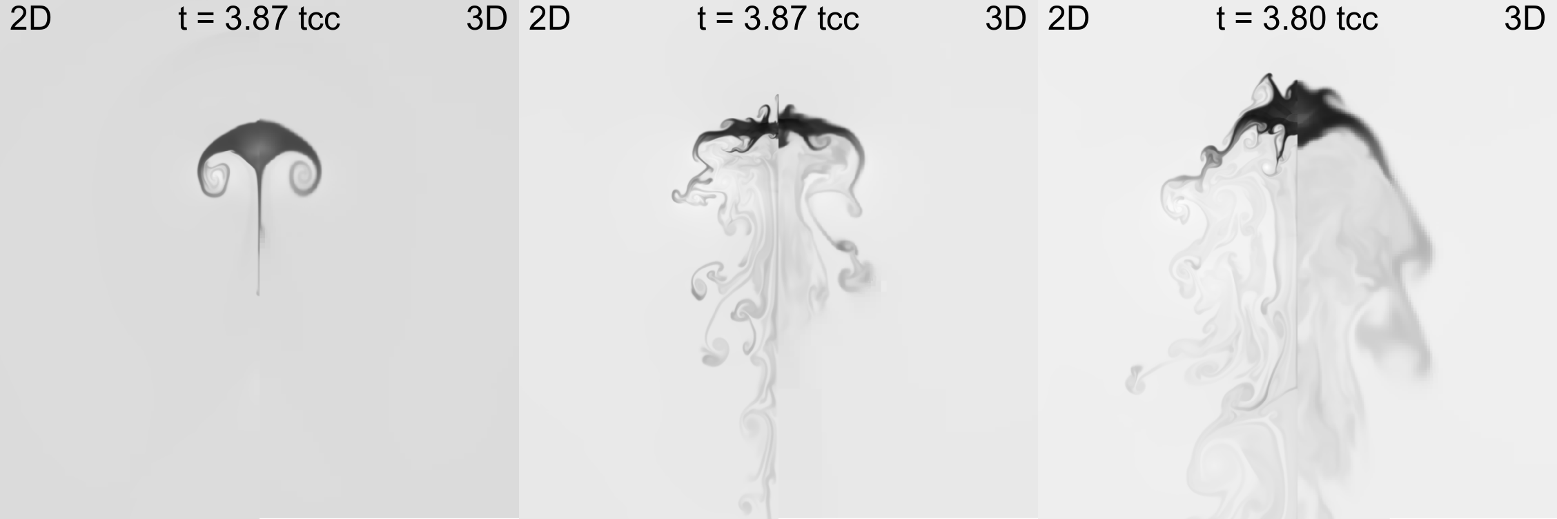
Figure 13: Comparison of 2D and 3D simulations for $M=1.5$. Left: $\chi=10$; Middle: $\chi=10^{2}$; Right: $\chi=10^{3}$. Each frame shows the region $-2<X<10$, $0<Y<6$. Note that each 2D simulation is at resolution $R_{128}$, while the 3D simulations are at the lower resolutions of $R_{64}$ ($\chi=10$) and $R_{32}$ ($\chi=10^{2}$ and $10^{3}$).

4.2 Statistics

Fig. 14 shows the evolution of $m_{\rm core}$ as a function of $M$ and $\chi$ for 2D and 3D simulations, with and without the subgrid turbulence model. This figure reveals that the 2D and 3D calculations are generally in very good agreement with each other. The most obvious differences occur between the $M=1.5$, $\chi=10$ simulations. The $M=3$, $\chi=10^{3}$, 2D $k$-$\epsilon$ simulation shown in panel f) is also surprisingly different from the others. Examination of this simulation shows that it proceeds similarly to the others, but that at later times the cloud and its core remains more compact than in the 2D inviscid or the 3D calculations. This ultimately leads to slower ablation and acceleration. It is not obvious why the cloud behaves so differently in this case, but we note similar behaviour in a 3D simulation at resolution $R_{32}$, which is examined in more detail in the appendix. The 4 models are most closely aligned when $\chi=10^{2}$ (for all $M$), and agreement is also good for the $M=10$, $\chi=10$ simulations. It is also interesting that the core is destroyed noticeably quicker in 3D simulations when $M=3$ and $\chi=10^{3}$.

Previously, Nakamura et al. (2006) reported that global quantities from a single 3D simulation of a shock striking a relatively hard-edged cloud ($n=8$) with $M=10$, $\chi=10$, at resolution $R_{60}$, are within 10% of an equivalent 2D calculation for $t<10\,t_{\rm cc}$ (see their Sec. 9.2.2). In Figs. 14-18 we compare our 2D and 3D results against each other. Examination of panel g) in Figs. 14-18 reveals that our 2D and 3D simulations are comparably similar for such parameters.

Fig. 15 shows the acceleration of the cloud. Good agreement between the simulations is again seen, with the 2D $M=3$, $\chi=10^{3}$ $k$-$\epsilon$ simulation again significantly discrepant. Clouds appear to generally be accelerated marginally faster in 3D calculations compared to 2D calculations when $\chi$ is high. This is caused by a faster and/or greater increase in the transverse radius of the cloud in 3D simulations (see Fig. 16). In contrast, the acceleration of clouds in the 3D simulations appears to be slightly slower when $\chi$ is low (particularly for $M=3$). Again, this appears to be related to differences in the transverse radius of the cloud. Xu & Stone (1995) note that their average cloud velocity reaches 0.85 of the postshock velocity (so $0.64v_{\rm b}$) by $t\approx 4\,t_{\rm cc}$ for M=10, $\chi=10$, so our results are in good agreement with theirs.

Fig. 17 shows the evolution of the transverse cloud velocity dispersion, $\delta v_{\rm r,cloud}$. Of note is that $\delta v_{\rm r,cloud}$ is almost always greater in the inviscid simulations than in simulations that use the subgrid turbulence model. This is irrespective of the dimensionality, and likely indicates the damping of velocity motions by the turbulent viscosity in the subgrid model. Again the $M=3$, $\chi=10^{3}$ $k$-$\epsilon$ simulation is noticeably discrepant.

The longitudinal velocity dispersion of the cloud is shown in Fig. 18. The simulation results are broadly comparable, but for low to moderate $M$ and moderate to high $\chi$, $\delta v_{\rm z,cloud}$ appears to peak higher and decay more slowly in the 2D simulations. This behaviour may be related to the lower resolution used in the 3D simulations in this region of parameter space.

Fig. 19 summarizes the Mach and density contrast dependence of the 3D inviscid results. These results can be compared against the 2D $k$-$\epsilon$ results in Figs. 5, 8 and 9 in Pittard et al. (2010). The same behaviour is seen but there are some qualitative differences. Compared to the 2D results, the 3D behaviour of $a_{\rm cloud}$ at $\chi=10^{3}$ shows much more variation with $M$. The major difference concerning the behaviour of $m_{\rm core}$ is the much less rapid ablation of the cloud when $M=1.5$ and $\chi=10$ in the 3D simulation compared to that in the 2D simulation.

Fig. 20 takes the results in Fig. 19 and plots them on a dimensionless timescale based on the post-shock velocity. Since the mixing and acceleration of the cloud is driven by the velocity gradients in the post-shock flow, we see that the data collapses to a tighter trend. This extends the behaviour previously noted by Niederhaus et al. (2008) to higher $\chi$ and $M$.

Fig. 21 also shows the variation of $c_{\rm cloud}$ and $c_{\rm cloud}/a_{\rm cloud}$ for the 3D inviscid calculations. As previously noted by Pittard et al. (2010), a long “tail-like” feature is formed only when $\chi\mathrel{\hbox to0.0pt{\lower 3.0pt\hbox{$\sim$}\hss}\raise 2.0pt\hbox{$>$}}10^{3}$. Comparison of $a_{\rm cloud}$, $c_{\rm cloud}$ and $c_{\rm cloud}/a_{\rm cloud}$ with Fig. 4 in Xu & Stone (1995) reveals good agreement for $M=10$ and $\chi=10$.

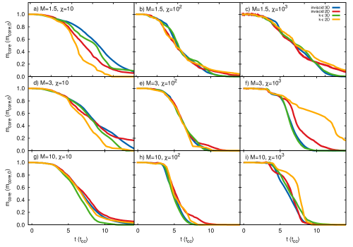
Figure 14: Comparison of the time evolution of the normalized core mass, $m_{\rm core}/m_{\rm core,0}$, for 2D (red and yellow) and 3D (blue and green) simulations with $M=1.5,3$ and 10 (top, middle and bottom panels, respectively), and $\chi=10,10^{2}$ and $10^{3}$ (left, centre and right panels, respectively). Results from inviscid and $k$-$\epsilon$ simulations are shown. Note the difference in the time-scale for the top panels (tick marks are at intervals of $5\,t_{\rm cc}$). The resolution of each of the 3D calculations is noted in Table 3. All the 2D calculations were performed at resolution $R_{128}$.

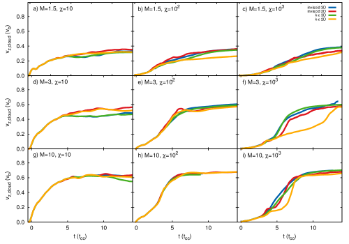
Figure 15: As Fig. 14 but showing the time evolution of the mean cloud velocity, $<v_{\rm z,cloud}>$.

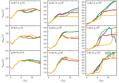
Figure 16: As Fig. 14 but showing the time evolution of the effective transverse radius of the cloud, $a_{\rm cloud}$.

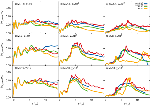
Figure 17: As Fig. 14 but showing the time evolution of the cloud velocity dispersion in the radial direction, $\delta v_{\rm r,cloud}$.

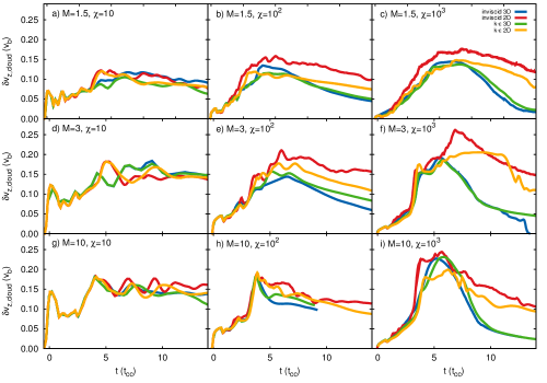
Figure 18: As Fig. 14 but showing the time evolution of the cloud velocity dispersion in the axial direction, $\delta v_{\rm z,cloud}$.

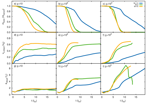
Figure 19: The time evolution of the normalized core mass, cloud mean velocity, and cloud transverse radius as a function of Mach number and cloud density contrast, for 3D inviscid simulations.

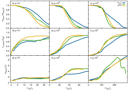
Figure 20: As Fig. 19, but plotting on the dimensionless timescale $tv_{\rm ps}/r_{\rm c}$. $v_{\rm z,cloud}$ is also scaled to the post-shock velocity, $v_{\rm ps}$.

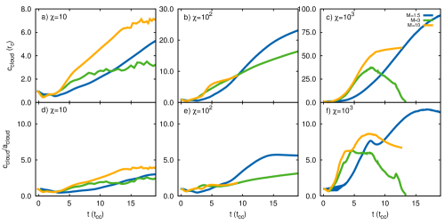
Figure 21: The time evolution of the cloud axial radius and shape as a function of Mach number and cloud density contrast, for 3D inviscid simulations.

Table 4: Various timescales (in units of $t_{\rm cc}$) calculated from the 3D inviscid simulations.

$\chi$	$M$	$t_{\rm drag}$	$t_{\rm drag,KMC}$	$t_{\rm mix}$	$t_{\rm life}$
10	1.5	3.14	8.65	16.4	$>30$
	3	1.36	3.86	8.42	16.6
	10	0.98	2.69	6.89	15.4
$10^{2}$	1.5	6.85	13.3	9.97	26.1
	3	3.65	5.38	6.00	12.8
	10	3.06	4.03	4.95	9.50
$10^{3}$	1.5	9.79	14.8	12.8	28.4
	3	5.13	6.57	6.31	10.7
	10	4.55	6.18	6.10	10.4

4.3 Timescales

Values of $t_{\rm drag}$, $t_{\rm mix}$ and $t_{\rm life}$ are noted in Table 4. In all cases $t_{\rm drag}<t_{\rm mix}<t_{\rm life}$ (though sometimes $t_{\rm drag,KMC}>t_{\rm mix}$). Fig. 22 shows the values of $t_{\rm drag}$, $t_{\rm mix}$ and $t_{\rm life}$ as a function of $M$ and $\chi$ for the 3D inviscid simulations. Also shown are the corresponding values from the 2D $k$-$\epsilon$ simulations in Pittard et al. (2010) and the fits made to this latter data. There is more scatter in $t_{\rm drag}$ and $t_{\rm mix}$ when $\chi=10^{3}$ due to spontaneous and random fragmentation.

Excellent agreement is found between the 2D and 3D results for $t_{\rm drag}$ when $\chi=10$ and 100, but clouds with $\chi=10^{3}$ accelerate more rapidly in the 3D calculations when $M\mathrel{\hbox to0.0pt{\lower 3.0pt\hbox{$\sim$}\hss}\raise 2.0pt\hbox{$>$}}3$. Since in the strong shock limit $t_{\rm drag}/t_{\rm cc}\propto\chi^{1/2}$ (see Eq. 9 in Pittard et al., 2010), one wonders whether the lower than expected drag time for the $M=10$, $\chi=10^{3}$ 3D simulation is a result of the lower resolution used. Alternatively, this may instead just be a result of the larger scatter when $\chi=10^{3}$ and the small number of simulations performed in 3D.

Xu & Stone (1995) postulated that clouds may be mixed more rapidly in 3D simulations due to the non-axisymmetric instabilities which develop, but this has not been tested prior to this work. We have already shown generally good agreement between our 2D and 3D calculations, both in terms of the morphology, and in terms of various global quantities. Fig. 14 shows that this is the case for $m_{\rm core}$, and Fig. 22 now lends further support by revealing that the 2D and 3D results have similar values of $t_{\rm mix}$ for $\chi=10^{2}$ and $10^{3}$. However, there is one set of simulations which stand out: for $M=1.5$ and $\chi=10$ it seems that the cloud takes longer to mix in the 3D simulations. Similar behaviour is found for $t_{\rm life}$. Fig. 14 shows that $m_{\rm core}$ declines increasingly slowly at late times in the 3D inviscid simulation, whereas in the 2D $k$-$\epsilon$ simulation $m_{\rm core}$ declines much more rapidly, reaching zero by $t\approx 20\,t_{\rm cc}$. Although not quite as rapid, the 2D inviscid simulation also has $m_{\rm core}$ declining faster than the 3D simulations.

Fig. 23 examines the 2D and 3D inviscid simulations side-by-side. It is clear that secondary vortices form earlier and are more prevelant in the higher resolution 2D simulation, and this may be the cause of the faster decline in $m_{\rm core}$. We also raise the possibility that the subgrid turbulence model is perhaps overly efficient at mixing the core material into low Mach number flows, given that the 2D inviscid simulation shows a slightly less rapid decline in $m_{\rm core}$ (see Fig. 14).

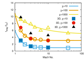
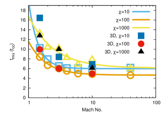
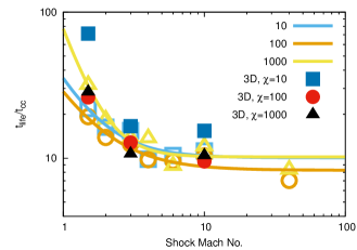
Figure 22: Top: $t_{\rm drag}$ (for the cloud); middle: $t_{\rm mix}$; and bottom: $t_{\rm life}$, as functions of the Mach number $M$ and cloud density contrast $\chi$. The 2D results are plotted using the open symbols, and fits to the 2D data are also shown (cf. Pittard et al., 2010).

Figure 23: As Fig. 2 but for the $M=1.5$, $\chi=10$ simulations. The first 2 frames show the same region ($-2<X<6$, $0<Y<4$ in units of $r_{\rm c}$) so that the motion of the cloud is clear. The other frames shift the $X$-axis to show $2<X<10$, $4<X<12$, and $9<X<17$ at $t=8.38$, 12.2, and $18.7\,t_{\rm cc}$, respectively. Note that the 2D simulation has a resolution of $R_{128}$, while the 3D simulation is at the lower resolution of $R_{64}$.

5 Conclusions

This is the third of a series of papers investigating the turbulent destruction of clouds. Our first paper (Pittard et al., 2009) noted the benefits of using a sub-grid turbulence model in simulations of shock-cloud interactions and found that clouds could be destroyed more rapidly when overrun by a highly turbulent flow. The inviscid and $k$-$\epsilon$ simulations were found to be in good agreement when the cloud density contrast $\chi\mathrel{\hbox to0.0pt{\lower 3.0pt\hbox{$\sim$}\hss}\raise 2.0pt\hbox{$<$}}100$, but they became increasingly divergent as $\chi$ increased. The $k$-$\epsilon$ simulations also displayed significantly better convergence properties, such that $\sim 30$ grid cells per cloud radius is needed for reasonable convergence (compared to the $\sim 120$ needed in inviscid simulations).

Our second paper (Pittard et al., 2010) investigated how the nature of the interaction changed with the Mach number $M$ and density contrast $\chi$. For $M\mathrel{\hbox to0.0pt{\lower 3.0pt\hbox{$\sim$}\hss}\raise 2.0pt\hbox{$>$}}7$, the lifetime of the cloud, $t_{\rm life}$, showed little variation with $M$ or $\chi$ and we found that $t_{\rm life}\sim 10\,t_{\rm cc}$. Due to the gentler nature of the interaction, $t_{\rm life}$ increases significantly at lower Mach numbers. A popular analytical formula for the mass-loss rate due to hydrodynamic ablation (Hartquist et al., 1986) was shown to predict cloud lifetimes which were inconsistent with Mach scaling and which had a $\chi$ dependence which was not supported by the simulation results.

In this third paper we have examined whether the conclusions in Pittard et al. (2010) remain valid for three dimensional simulations, and whether the nature of the interaction is different in 2D axisymmetric and fully 3D simulations. This was motivated by previous reports that clouds are destroyed more rapidly in 3D due to the additional development of non-axisymmetric instabilites. However, our detailed investigation, covering Mach numbers from $1.5-10$ and cloud density contrasts from $10-10^{3}$, has instead revealed that the interaction proceeds very similarly in 2D and 3D. Although non-azimuthal modes lead to different behaviour in the later stages of the interaction, they have very little effect on key global quantities such as the lifetime of the cloud and its acceleration.

In particular, we are not able to confirm differences in the hollowing or “voiding” of the cloud between 2D and 3D simulations with $M=10$ and $\chi=10$. This contrasts with the findings in Klein et al. (2003), where 3D experimental data and 3D simulations display such voiding but synthetic shadowgrams based on 2D simulations do not. We note that the 2D and 3D simulations in Klein et al. (2003) are computed with different numerical codes and different initial conditions. Our work shows that when the same code and initial conditions are used the interaction evolves almost identically.

The biggest differences between our 2D and 3D simulations occur for $M=1.5$ and $\chi=10$ - the destruction is noticeably slower in 3D. It is not clear why this is so, though secondary vortices form earlier and are more prevelant in the higher resolution 2D simulations. Having said this, our resolution tests indicate that increasing the resolution of the 3D simulation is likely to slow the destruction of the cloud yet further (see Fig. 31). Additional 3D simulations at higher resolution are necessary to resolve this issue.

We have also shown how the cloud acceleration (through $t_{\rm drag}$) and mixing (through $t_{\rm mix}$) are affected by low resolution. We find that these timescales are up to $5\times$ shorter for clouds at resolution $R_{1}$ (i.e. very poorly resolved clouds). This is relevant to simulations of the mixing and entrainment of cold clouds in multiphase-flows: simulations which do not adequately resolve the cold clouds in the flow will underestimate $t_{\rm drag}$ and $t_{\rm mix}$, often to a significant degree.

Our work has also highlighted that 3D inviscid and $k$-$\epsilon$ simulations give typically very similar results. This is somewhat surprising given that 2D calculations can show significant differences (see Pittard et al., 2009, 2010), but must be related to the different way that vortices behave and evolve in 2D and 3D flows. Unlike in 2D, we find no evidence for convergence at lower resolution when employing the $k$-$\epsilon$ model. Hence, there seems to be no compelling reason to use the $k$-$\epsilon$ model in 3D calculations, but clearly it remains very useful in 2D calculations.

In future work we will examine the dependence of the interaction on the shape and orientation of the cloud, and in particular whether the nature of the interaction changes when the cloud is elongated/filamentary. By examining the destruction of spherical clouds in 3D, the present work has laid the necessary groundwork for this forthcoming study.

Appendix A Resolution Test

In an actual shock-cloud interaction, the smallest instabilities have a length scale, $\eta$, which is set by the damping of hydromagnetic waves. This is typically through particle collisions, but can also be through wave-particle interactions (see Sec. 2.2 of Pittard et al., 2009), and is dependent on the nature of the problem. For instance, in astrophysical problems it depends on whether the cloud is ionized, neutral or molecular, and the strength of the magnetic field and thermal conductivity. The Reynolds number of a flow past a cloud is ${\rm Re}=ur_{\rm c}/\nu$, where $u$ is the average flow speed past the cloud, $r_{\rm c}$ is the radius of the cloud, and $\nu$ is the kinematic viscosity. For astrophysical scenarios, Re can easily exceed a value of $10^{5-6}$ (Pittard et al., 2009). The size of the smallest eddies, $\eta\sim{\rm Re}^{-3/4}l$, where the largest eddies have a length scale, $l$, comparable in size to the cloud. Resolving the smallest eddies in a numerical simulation can thus be very challenging. Alternatively, a $k$-$\epsilon$ model can be used to explicitly model the effects of sub-grid-scale turbulent viscosity through the addition of turbulence-specific viscosity and diffusion terms to the Euler equations (Pittard et al., 2009, 2010).

Without any prescription for the small-scale dissipative physics, new unstable scales will be added as the resolution of the simulation is increased. This is the case for simulations which simply solve the Euler equations for inviscid fluid flow. For instance, simulations of a shock striking a cloud will produce features which depend on the resolution adopted. Higher resolution simulations allow the development of smaller instabilities, and surfaces and interfaces become sharper. These differences can affect the rate at which material is stripped from the cloud and mixed into the surrounding flow, and the acceleration that the cloud experiences. Increasing the resolution simply creates finer and finer structure as Re increases. In the shock-cloud scenario, the different instabilities present at different resolution will break up the cloud differently, thus eventually affecting the convergence of integral quantities. Thus formal convergence may be impossible in “inviscid” simulations. Samtaney & Pullin (1996) have shown that initial value problems for the Euler equations involving shock-contact interactions exhibit features indicating that such problems are ill-posed, including non-convergence of the solution at a given time.

Simulations of problems for which there is no analytical solution typically rely on a demonstration of self-convergence. Lower resolution simulations are compared against the highest resolution simulation performed, and a resolution is chosen which balances accuracy against computational cost. Klein et al. (1994) suggested that $\sim 100$ cells per cloud radius was required to adequately model the adiabatic interaction of a Mach 10 shock with a $\chi=10$ cloud. Most simulations in the astrophysics literature since then have adopted resolutions matching or exceeding this requirement, though some 3D studies have been performed at lower resolution. More recently, Niederhaus et al. (2007) examined the issue of convergence for 2D calculations of the purely adiabatic interaction of a shock with a spherical cloud. They find that although the solution is locally and pointwise nonconvergent, some aspects of the computed flowfields, particularly certain integrated and mean quantities, do reach a converged grid-independent state. For instance, they show that the maximum density in the flowfield continues to vary with the spatial resolution (even for resolutions up to $R_{1024}$), while the mean cloud density converges to a nearly grid-independent value for resolutions $>R_{500}$.

At very low resolution, important features of the flow may not be present, and ultimately the simulated interaction will compare poorly to reality. Thus, rather than attempting to obtain a converged solution, some previous work has instead focussed on resolving key features of the flow. In purely hydrodynamic shock-cloud simulations this includes the stand-off distance of the bowshock (e.g., Farris & Russell, 1994) and the thickness of the turbulent boundary layer on the cloud surface (see Pittard et al., 2009, and references therein); in radiative shock-cloud simulations it is the cooling layer behind shocks (Yirak et al., 2010), while in the MHD simulations of Dursi & Pfrommer (2008) it is the magnetic draping layer on the upstream surface of the cloud.

To understand how the grid resolution affects our results we have run a variety of simulations at different resolutions, with and without inclusion of a $k$-$\epsilon$ sub-grid model. In the following subsections we examine the resolution dependence of the cloud morphology, study some statistics of the interaction, determine how certain integral quantities vary with resolution, and finally study the impact of resolution on the cloud acceleration and mixing timescales, $t_{\rm drag}$ and $t_{\rm mix}$.

Figure 24: Comparison with resolution of the “inviscid” $M=10$, $\chi=10$ simulation at $t=4.09\,t_{\rm cc}$. From top to bottom the resolutions are $R_{8},R_{16},R_{32},R_{64}$ and $R_{128}$.

A.1 Cloud Morphology

We first study the resolution dependence of the cloud morphology for “inviscid” simulations with $M=10$ and $\chi=10$, which are the most popular parameter choices in the astrophysical literature to date (see Table 1). We expect the bowshock to have a stand-off distance of $\approx 0.28\,r_{\rm c}$ (Farris & Russell, 1994). Hence the bowshock will be resolved at resolutions $\mathrel{\hbox to0.0pt{\lower 3.0pt\hbox{$\sim$}\hss}\raise 2.0pt\hbox{$>$}}R_{16}$, while resolving the turbulent boundary layer requires resolutions $\sim R_{100}$.

Fig. 24 shows volumetric plots of the density of cloud material at $t=4.09\,t_{\rm cc}$ (this focus means that features in the ambient medium - e.g., the bowshock - are not visible). As the resolution increases we see that the shape of the cloud changes, from rounded and relatively featureless at lower resolutions, to displaying a torus of high vorticity at the highest resolutions. The cloud and the vortex ring at the rear of the cloud are merged together in the $R_{8}$ simulation, but become increasingly separate and distinct as the resolution increases. At $R_{64}$ numerous density structures occur within the cloud interior (these are not readily visible in Fig. 24, but are clearly identifiable when this figure is rotated on the computer screen), which break up into smaller structures in the $R_{128}$ simulation (these are clearly visible in the 2D slices shown in Fig. 2). At $R_{64}$ the vortex ring shows azimuthal variations for the first time. In addition, the thickness of the slip surface decreases and the maximum density of cloud material increases as the resolution increases.

Fig. 25 shows the resolution-dependent behaviour of simulations with $M=10$, $\chi=10^{2}$. It is interesting to see how the dominant scale of the instabilities changes with resolution. For $R_{8}$, $R_{16}$ and $R_{32}$, the cloud has 4 dominant fingers. At $R_{64}$ and $R_{128}$ smaller scale structures develop which change these fingers into a single ring-like feature. The main effect of the resolution in “inviscid” simulations is to set the size of the instabilities which develop: at low resolution only longer-wavelength instabilities can develop. The tail appears to display some characteristics of turbulence at $R_{64}$ and above.

Fig. 26 shows volumetric plots of the cloud density at $t=0.79\,t_{\rm cc}$ for the $M=10$, $\chi=10^{3}$ simulations as a function of the resolution. As the resolution increases we again see that the thickness of the slip surface decreases and the maximum density of the shocked cloud increases. The tail of ablated material also becomes more hollow, and its shape changes. At the highest resolution studied the tail is disrupted by instabilities after about 3 cloud radii, and becomes “turbulent”. At this time very little material has been stripped from the cloud but there are already important qualitative and quantitative differences in the flow.

Fig. 27 shows the resolution dependent morphology at a later time ($t=3.80\,t_{\rm cc}$). Despite the dramatic changes to the shape of the cloud, the core has yet to suffer significant mass loss. As expected, the differences with resolution are much more pronounced than in Fig. 26. At $R_{8}$ the cloud has 4 dominant fingers while at $R_{16}$ a central finger is also seen. At $R_{32}$ and $R_{64}$ we instead find that the bulk of the cloud material forms a coherent structure located on the original cloud axis. At these later times we see similar changes with resolution as for the $M=10$, $\chi=10^{2}$ simulations discussed previously.

Fig. 28 examines how the resolution affects simulations with $\chi=10^{2}$ when the Mach number of the shock is lowered to $M=1.5$. At $R_{8}$ the cloud is reasonably featureless. At $R_{16}$ a small “bump” is visible on the leading surface, and the cloud becomes both somewhat hollow and also less extended in the axial direction. In the $R_{32}$ simulation the leading “bump” is more extended, and in the $R_{64}$ simulation it splits into 4 parts. We identify these features as RM instabilities (cf. Fig 1 in Stone & Norman, 1992). The remainder of the cloud has an appearance which resembles a “jelly-fish” at the highest resolution examined.

In terms of the morphology, the general impression that one gets from Figs. 24-28 is that $R_{64}$ is the minimum resolution needed to capture the morphology accurately in a qualitative sense. Our investigation is therefore consistent with the statement in Xu & Stone (1995) that $R_{60}$ “has captured the dominant dynamical effects present in the evolution”.

Figure 25: Comparison with resolution of the $M=10$, $\chi=10^{2}$ simulation at $t=3.87\,t_{\rm cc}$. From left to right and top to bottom the resolutions are $R_{8},R_{16},R_{32},R_{64}$ and $R_{128}$.

Figure 26: Comparison with resolution of the $M=10$, $\chi=10^{3}$ simulation at $t=0.79\,t_{\rm cc}$. From left to right and top to bottom the resolutions are $R_{8},R_{16},R_{32}$ and $R_{64}$. The initial cloud density is 1000.

Figure 27: As Fig. 26 but at $t=3.80\,t_{\rm cc}$.

Figure 28: Comparison with resolution of the $M=1.5$, $\chi=10^{2}$ simulation at $t=3.87\,t_{\rm cc}$. From left to right and top to bottom the resolutions are $R_{8},R_{16},R_{32}$, and $R_{64}$.

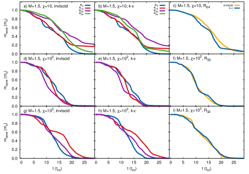
Figure 29: Time evolution of the core mass, $m_{\rm core}$, for simulations with $M=1.5$. The top row has $\chi=10$, the middle row has $\chi=10^{2}$, and the bottom row has $\chi=10^{3}$. The calculations are made at various resolutions for inviscid (left column) and k-$\epsilon$ (middle column) simulations. A comparison at the indicated resolution is made between the inviscid and k-$\epsilon$ results in the right column.

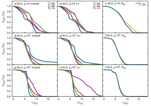
Figure 30: As Fig. 29 but for $M=3$.

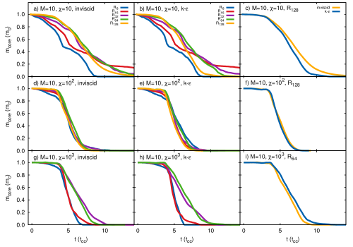
Figure 31: As Fig. 29 but for $M=10$.

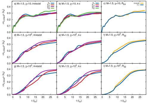
Figure 32: Time evolution of the cloud velocity, $<v_{\rm z,cloud}>$, for simulations with $M=1.5$. The top row has $\chi=10$, the middle row has $\chi=10^{2}$, and the bottom row has $\chi=10^{3}$. The calculations are made at various resolutions for inviscid (left column) and k-$\epsilon$ (middle column) simulations. A comparison at the indicated resolution is made between the inviscid and k-$\epsilon$ results in the right column.

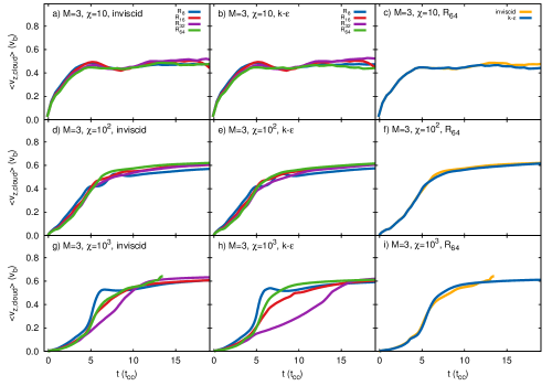
Figure 33: As Fig. 32 but for $M=3$.

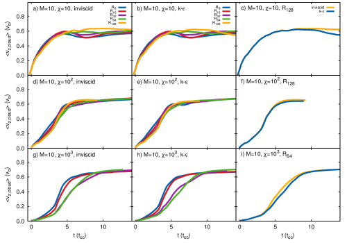
Figure 34: As Fig. 32 but for $M=10$.

A.2 Time Evolution

Figs. 29-31 show the time evolution of the core mass, $m_{\rm core}$, for 3D simulations with $\chi=10,10^{2}$ and $10^{3}$ and $M=1.5,3$ and 10. In each figure, the left panels (a, d and g) show results at different resolutions from the “inviscid” calculations, while the centre panels (b, e and h) show corresponding results from the $k$-$\epsilon$ calculations. The right panels (c, f and i) compare the highest resolution simulations from each of these models. In a similar fashion, Figs. 32-34 show the time evolution of the mean cloud velocity, $<v_{\rm z,cloud}>$, for the same runs. Since the displayed profiles are generally less disparate and show a tighter correlation for the cloud velocity than for the core mass we will concentrate on the latter in the following discussion.

Consider first the $M=10$ results (see Fig. 31). For $\chi=10$ and $\chi=10^{3}$ it is clear that there are very large differences in the time dependent behaviour of $m_{\rm core}$ between simulations at resolutions below $R_{32}$. However, for both values of $\chi$ the $R_{32}$ and $R_{64}$ simulations are reasonably matched. This is true for both the “inviscid” and $k$-$\epsilon$ cases. Surprisingly, the simulations for $\chi=10^{2}$ are much less dependent on resolution. In all cases, the clouds in simulations with higher resolutions lose core mass initially more slowly, but then show more rapid core mass loss at later times (this is particularly true for the $\chi=10$ simulations). The former is due to the higher numerical viscosity and thickness of the shear layer, while the latter is caused by the larger dynamic range of instabilities which eventually develop. The important point is that simulations with a resolution of $R_{32}$ appear to show that the time evolution of $m_{\rm core}$ and $<v_{\rm z,cloud}>$ are reasonably converged.

In contrast, 2D axisymmetric simulations of an adiabatic shock striking a spherical cloud have $m_{\rm core}$ and $<v_{\rm z,cloud}>$ profiles which do not converge until $\sim R_{128}$ for “inviscid” calculations (see, e.g., Fig. 2 in Pittard et al., 2009). That the resolution requirement for 3D calculations is lower than for 2D calculations is likely due to the fundamentally different behaviour of 2D versus 3D turbulence (e.g., the absence of vortex-stretching in 2D, and the transport of kinetic energy from large to small scales in 3D (and vice-versa in 2D)). This behaviour indicates that fully 3D simulations better represent the actual flow, and can “outperform” 2D simulations of higher resolution (at least for the behaviour of $m_{\rm core}$ and $<v_{\rm z,cloud}>$ - further work is necessary to see if this is true for other integrated quantities and for the flow field in general). On the other hand, it remains the case that higher resolution simulations will develop smaller scale instabilities, and that one can expect that resolutions in excess of $R_{32}$ will be needed for the convergence of other properties, such as minimum and maximum quantities (cf. Niederhaus et al., 2007).

Another surprise is that we see little difference between the inviscid and $k$-$\epsilon$ 3D simulations. In particular, there is no indication that the $k$-$\epsilon$ simulations converge at a lower resolution than their inviscid counterparts (see Fig. 31). This is in contrast to the 2D simulation results presented in Pittard et al. (2009), where a major finding was that the $k$-$\epsilon$ simulations converged at significantly lower resolutions (roughly $R_{32}$) than their inviscid counterparts (roughly $R_{128}$). It seems that the ability of instabilities to grow in any direction means that 3D calculations more accurately capture the real behaviour of such systems whether or not a $k$-$\epsilon$ model is used. Thus there seems to be little benefit in employing the $k$-$\epsilon$ model in 3D shock-cloud simulations (though its lower resolution requirements for convergence mean that it remains useful for 2D simulations).

For completeness we consider the resolution-dependent behaviour of 3D simulations with a shock Mach number $M=3$ (Figs. 30 and 33) and $M=1.5$ (Figs. 29 and 32). The same general behaviour is seen in the $M=3$ simulations as in the $M=10$ simulations and thus the same broad conclusions can be drawn (e.g., $R_{32}$ is roughly the minimum needed for $m_{\rm core}$ and $<v_{\rm z,cloud}>$ to be reasonably converged).

The only significant discrepancy between the inviscid and $k$-$\epsilon$ simulations occurs when $M=3$ and $\chi=10^{3}$ - the $R_{32}$ $k$-$\epsilon$ simulation appears at odds with the others. Fig. 35 compares the morphology of the inviscid and $k$-$\epsilon$ as a function of resolution at a number of different times. Panels a) and b) show that the nature of the interaction and the way the cloud is destroyed depends strongly on the resolution. However, apart from a “smoother” wake in the $k$-$\epsilon$ models, the cloud morphology is otherwise almost identical between panels a) and b). The major difference is that the cloud has a much more compact cross-section in the $R_{32}$ calculations at $t=5.73\,t_{\rm cc}$. It is not obvious from the preceding panels why this occurs. It is at about this time that the core mass and mean cloud velocity in the $R_{32}$ $k$-$\epsilon$ simulation start to diverge from the other models (see Figs. 30 and 33). In the inviscid simulation, the cloud is already showing some asymmetry at $t=5.73\,t_{\rm cc}$. This becomes more pronounced at later times, as shown in Fig. 35c), and the cloud develops significant transverse motions which speeds up its mixing and acceleration. In contrast, in the $k$-$\epsilon$ simulation the cloud remains compact and symmetrical to very late times. As such, its core mass drops more slowly as it suffers less ablation, and its acceleration is much slower. This behaviour accounts for the differences seen in Figs. 30 and 33. It highlights the fact that instabilities develop differently at different resolutions, and supports our earlier statement that this can eventually influence the global mixing and acceleration of cloud material.

High resolutions, particularly at high cloud density contrasts, are very computationally demanding when $M=1.5$ because of the gentler nature of the interaction and the longer run times which ensue. For this reason we were unable to perform calculations above $R_{64}$ for $\chi=10^{2}$, and above $R_{32}$ for $\chi=10^{3}$. We note that $m_{\rm core}$ and $<v_{\rm z,cloud}>$ appear reasonably converged for $R_{32}$ and $R_{64}$ when $M=1.5$ and $\chi=10$. However, further work is needed to determine whether $R_{32}$ is an adequate resolution for $m_{\rm core}$ and $<v_{\rm z,cloud}>$ $M=1.5$ when $\chi\mathrel{\hbox to0.0pt{\lower 3.0pt\hbox{$\sim$}\hss}\raise 2.0pt\hbox{$>$}}100$.

The only published resolution test for 3D hydrodynamic simulations that we are aware of in the astrophysics literature is shown in Fig. 5 of Xu & Stone (1995). They plot the time evolution of a number of cloud properties, including $m_{\rm core}$ and $<v_{\rm z,cloud}>$, for simulations with $M=10$ and $\chi=10$, with 11, 25 and 53 cells per cloud radius. They find smaller differences between the $R_{25}$ and $R_{53}$ simulations, than between the $R_{11}$ and $R_{25}$ simulations, and thus claim that their highest resolution simulation captures the dominant dynamical effects. Our work is consistent with these claims.

Figure 35: Comparison of the 3D $M=3$, $\chi=10^{3}$ simulations with time and resolution in the $Z=0$ plane. A grayscale of the logarithmic density is shown between $\rho_{\rm amb}$ (white) and $4\times\rho_{\rm c}$ (black). a) Inviscid models. b) $k$-$\epsilon$ models. In both a) and b), results at resolutions $R_{16}$ (top), $R_{32}$ (middle), and $R_{64}$ (bottom) are shown. c) At later times the $R_{32}$ inviscid (top) and $k$-$\epsilon$ (bottom) simulations are compared. The frames show the region ($0<X<12$, $-3<Y<3$) at $t=2.51$ and $3.15\,t_{\rm cc}$, ($0<X<20$, $-5<Y<5$) at $t=3.80\,t_{\rm cc}$, ($0<X<26$, $-6.5<Y<6.5$) at $t=5.73\,t_{\rm cc}$, and ($0<X<50$, $-7<Y<7$) at $t=7.67$ and $11.5\,t_{\rm cc}$ (all in units of $r_{\rm c}$). Note that in this figure the $X$-axis is plotted horizontally.

A.3 Convergence Tests

To gain further insight into the effect of the grid resolution on our simulations we examine the variation of some integral quantities computed from the datasets. One method for examining the degree of convergence between simulations at different resolution is to study the relative error, which is defined as the fractional difference between the value measured at resolution $N$ and the value at the finest resolution, $f$:

$$\Delta Q_{N}=\frac{|Q_{N}-Q_{f}|}{|Q_{f}|}.$$ (5)

If $\Delta Q_{N}$ shows a monotonic decrease with increasing resolution, and is small, then self-convergence is occurring (e.g., Yirak et al., 2010). This behaviour translates into an asymptotic levelling off with increasing resolution of a particular quantity.

However, there is also the danger of “false convergence”, whereby further increases in resolution show that the models actually have not converged (see, e.g., Fig. 10a in Niederhaus et al., 2007). This can happen when an important flow feature is resolved for the first time (e.g., the standoff of the bowshock, or the cooling zone of radiative shocks). Furthermore, simulations which demonstrate convergence at a particular simulation time may well not be converged at a later time. This is expected for simulations of the “inviscid” Euler equations, where RT and KH instabilities in simulations at different resolution will break up the cloud differently, thus eventually affecting the convergence of integral quantities. Therefore, any statement that such simulations are “converged” must be qualified by a time, and by the caveat that this does not imply that convergence exists at later times.

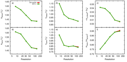
Figure 36: Integral quantities from the $M=10$, $\chi=10$, simulations at $t=3.14\,t_{\rm cc}$, plotted as a function of the grid resolution.

The variation in $a_{\rm cloud}$, $c_{\rm cloud}$, $<v_{\rm z,cloud}>$, $a_{\rm core}$, $c_{\rm core}$ and $m_{\rm core}$ with the spatial resolution for the $M=10$, $\chi=10$ 3D inviscid and $k$-$\epsilon$ simulations is shown in Fig. 36. We again notice the very good agreement between the inviscid and $k$-$\epsilon$ simulations. We also see that some quantites appear to be converged ($c_{\rm core}$), some appear to show signs of convergence ($a_{\rm cloud}$, $a_{\rm core}$ and $m_{\rm core}$), while some are clearly not converged ($c_{\rm cloud}$ and $<v_{\rm z,cloud}>$). Therefore, our simulations are not formally converged at this time. However, they are at sufficient resolution that some global quantities are. Clearly, it would be useful to extend this convergence study to still higher resolutions.

We are also interested in the variation of these integral quantities with resolution from simulations with a higher density contrast. Fig. 37 shows this behaviour for models with $M=10$ and $\chi=10^{3}$. We see that there is clear asymptotic levelling off of $c_{\rm cloud}$, $<v_{\rm z,cloud}>$, and $c_{\rm core}$ ($k$-$\epsilon$ only), indicating that the solutions are converging for these quantities. However, there is no levelling off for $a_{\rm core}$ and $a_{\rm cloud}$, indicating clear non-convergence. $m_{\rm core}$ may be showing signs of convergence, but more data is needed. We conclude that our simulations are again not formally converged, but it appears that the highest resolution simulations have sufficient resolution that some of the integral quantities are showing signs of convergence at this time.

Moving to later times ($t=6\,t_{\rm cc}$), Fig. 38 shows that none of the quantities (except perhaps $a_{\rm core}$) display any signs of convergence. This demonstrates that as the simulations advance in time they move from showing some convergence to showing non-convergence. Thus we can be totally clear that still higher resolution is necessary in order to obtain formal convergence (at $t\approx 3\,t_{\rm cc}$, let alone at later times), if indeed this is even possible given the nature of the inviscid Euler equations.

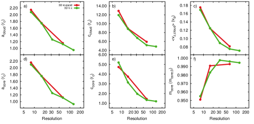
Figure 37: Integral quantities from the $M=10$, $\chi=10^{3}$, simulations at $t=2.9\,t_{\rm cc}$, plotted as a function of the grid resolution.

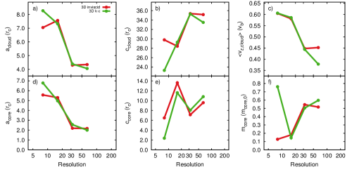
Figure 38: Integral quantities from the $M=10$, $\chi=10^{3}$, simulations at $t=6.0\,t_{\rm cc}$, plotted as a function of the grid resolution.

A.4 Timescales

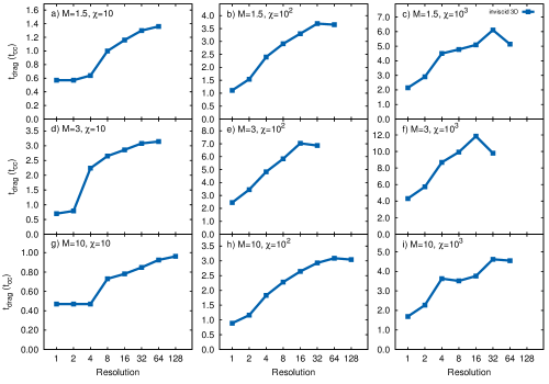
Figure 39: Resolution dependence of $t_{\rm drag}$ (for the cloud) as functions of the Mach number $M$ and cloud density contrast $\chi$.

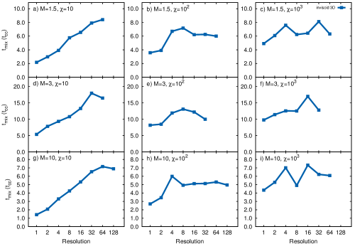
Figure 40: Resolution dependence of $t_{\rm mix}$ as functions of the Mach number $M$ and cloud density contrast $\chi$.

Figs. 39 and 40 examine the resolution dependence of $t_{\rm drag}$ and $t_{\rm mix}$. In general, $t_{\rm drag}$ increases with resolution. However, there are few signs of convergence towards an asymptote, so further resolution tests are needed to determine $t_{\rm drag}$ accurately. Since, $t_{\rm mix}>t_{\rm drag}$ in all cases, it is not surprising that we do not see formal convergence for $t_{\rm mix}$ either.

While formal convergence is not seen, in many cases $t_{\rm drag}$ and $t_{\rm mix}$ level-off at higher resolutions, indicating that their values may be reasonably close to the “true” value. It is also of interest to note by how much $t_{\rm drag}$ and $t_{\rm mix}$ are underestimated in lower resolution calculations. By averaging the values in Fig. 39 we find that $t_{\rm drag}$ is only 40% of its maximum resolution value at $R_{1}$, climbing to 83% at $R_{8}$ and 93% at $R_{16}$, and is on average within 1% of its maximum resolution value for $R_{32}$ and higher resolutions.

There is significantly more scatter in the resolution dependence of $t_{\rm mix}$, as shown in the bottom panel of Fig. 40. However, like $t_{\rm drag}$, there is a clear trend that $t_{\rm mix}$ is underestimated in lower resolution calculations. At $R_{1}$, $t_{\rm mix}$ is on average 56% of its value from our highest resolution simulations, and is on average 10% lower at $R_{8}$. In some simulations it can be only 20% of its true value, while in others it can be nearly 30% longer. Note that there is a tight correlation in the trend of $t_{\rm mix}$ when $\chi=10$, for the 3 Mach numbers investigated: at $R_{1}$ and $R_{8}$, $t_{\rm mix}$ is 26% and 64% of the true value, respectively.

Figs. 39 and 40 indicate that clouds will be accelerated and destroyed more rapidly than they should be when they are poorly resolved in numerical simulations. This has implications for simulations of a wide-range of multiphase flows, including the collision of stellar winds (Stevens et al., 1992; Walder & Folini, 2002; Pittard, 2007a; Pittard et al., 2009; Parkin et al., 2011), the interaction of stellar winds, jets and SNe with their local environment (e.g. Jun, Jones & Norman, 1996; Steffen & López, 2004; Tenorio-Tagle et al., 2006; Yirak et al., 2008; Rogers & Pittard, 2013; Dale et al., 2014), the SN-regulated ISM (e.g., de Avillez & Breitschwerdt, 2005; Joung & Mac Low, 2006; Joung et al., 2009; Hill et al., 2012; Kim et al., 2013; Creasey et al., 2013; Hennebelle & Iffrig, 2014; Walch et al., 2015; Girichidis et al., 2015), galactic outflows and superwinds (e.g., Strickland & Stevens, 2000; Cooper et al., 2008; Dubois & Teyssier, 2008; Ceverino & Klypin, 2009; Fujita et al., 2009; Hopkins et al., 2012; Marinacci et al., 2014; Schaye et al., 2015; Vorobyov et al., 2015; Kimm et al., 2015), ram-pressure stripping of the ISM from galaxies (e.g., Tonnesen & Bryan, 2009; Roediger et al., 2014; Vijayaraghavan & Ricker, 2015), and AGN feedback (e.g., Sutherland & Bicknell, 2007; Wagner et al., 2012). It also affects studies of the interaction of a shock with multiple clouds (e.g., Poludnenko et al., 2002; Melioli et al., 2005; Alūzas et al., 2012), and mass-loaded flows in general (see the review by Pittard, 2007b).

References

- Abdo et al. (2010) Abdo A. A., et al., 2010, Science, 327, 1103
- Ackermann et al. (2013) Ackermann M., et al., 2103, Science, 339, 807
- Agertz et al. (2007) Agertz O., et al., 2007, MNRAS, 380, 963
- Alarie et al. (2014) Alarie A., Bilodeau A., Drissen L., 2014, MNRAS, 441, 2996
- Alūzas et al. (2012) Alūzas R., Pittard J. M., Hartquist T. W., Falle S. A. E. G., Langton R., 2012, MNRAS, 425, 2212
- Arthur & Henney (1996) Arthur, S. J., & Henney, W. J. 1996, ApJ, 457, 752
- Aschenbach et al. (1995) Aschenbach B., Egger R., Trumper J., 1995, Nature, 373, 587
- Blair et al. (2000) Blair W. P., et al., 2000, ApJ, 537, 667
- Brogan et al. (2013) Brogan C. L., et al., 2013, ApJ, 771, 91
- Bykov et al. (2008) Bykov A. M., 2008, ApJ, 676, 1050
- Cecil et al. (2001) Cecil G., Bland-Hawthorn J., Veilleux S., Filippenko A. V., 2001, ApJ, 555, 338
- Ceverino & Klypin (2009) Ceverino D., Klypin A., 2009, ApJ, 695, 292
- Chen & Slane (2001) Chen Y., Slane P. O., 2001, ApJ, 563, 202
- Chevalier & Kirshner (1979) Chevalier R. A., Kirshner R. P., 1979, ApJ, 233, 154
- Chièze & Lazareff (1981) Chièze, J. P., & Lazareff, B. 1981, A&A, 95, 194
- Childs et al. (2012) Childs H., et al., 2012, “VisIt: An End-User Tool For Visualizing and Analyzing Very Large Data”, in High Performance Visualization–Enabling Extreme-Scale Scientific Insight (eds. E. Wes Bethel, Hank Childs, Charles Hansen), p.357-372, CRC Press
- Close et al. (2013) Close J. L., Pittard J. M., Hartquist T. W., Falle S. .A. E. G., 2013, MNRAS, 436, 3021
- Cooper et al. (2008) Cooper J. L., Bicknell G. V., Sutherland R. S., Bland-Hawthorn J., 2008, ApJ, 674, 157
- Cowie et al. (1981) Cowie, L. L., McKee, C. F., & Ostriker, J. P. 1981, ApJ, 247, 908
- Creasey et al. (2013) Creasey P., Theuns T., Bower R. G., 2013, MNRAS, 429, 1922
- Dale et al. (2014) Dale J. E., Ngoumou J., Ercolano B., Bonnell I. A., 2014, MNRAS, 442, 694
- de Avillez & Breitschwerdt (2005) de Avillez M. A., Breitschwerdt D., 2005, A&A, 436, 585
- Dubois & Teyssier (2008) Dubois Y., Teyssier R., 2008, A&A, 477, 79
- Dursi & Pfrommer (2008) Dursi L. J., Pfrommer C., 2008, ApJ, 677, 993
- Dyson et al. (2002) Dyson, J. E., Arthur, S. J., & Hartquist, T. W. 2002, A&A, 390, 1063
- Elmegreen & Scalo (2004) Elmegreen B. G., Scalo J., 2004, ARA&A, 42, 211
- Elmhamdi et al. (2004) Elmhamdi A., Danziger I. J., Cappellaro E., Della Valle M., Gouiffes C., Phillips M. M., Turatto M., 2004, A&A, 426, 963
- Falle (1991) Falle S. A. E. G., 1991, MNRAS, 250, 581
- Farris & Russell (1994) Farris M. H., Russell C. T., 1994, J. Geophys. Research, 99, 17681
- Fassia et al. (1998) Fassia A., Meikle W. P. S., Geballe T. R., Walton N. A., Pollacco D. L., Rutten R. G. M., Tinney C., 1998, MNRAS, 299, 150
- Fesen & Kirshner (1980) Fesen R. A., Kirshner R. P., 1980, ApJ, 242, 1023
- Fesen (2001) Fesen R. A., Morse J. A., Chevalier R. A., Borkowski K. J., Gerardy C. L., Lawrence S. S., van den Bergh S., 2001, AJ, 122, 2644
- Fesen et al. (2011) Fesen R. A., Zastrow J. A., Hammell M. C., Shull J. M., Silvia D. W., 2011, ApJ, 736, 109
- Filippenko & Sargent (1989) Filippenko A. V., Sargent W. L. W., 1989, ApJ, 345, L43
- Finkelstein et al. (2006) Finkelstein S. L., et al., 2006, ApJ, 641, 919
- Fujita et al. (2009) Fujita A., Martin C. L., Mac Low M.-M., New K. C. B., Weaver R., 2009, ApJ, 698, 693
- Ghavamian et al. (2005) Ghavamian P., Hughes J. P., Williams T. B., 2005, ApJ, 635, 365
- Girichidis et al. (2015) Girichidis P., et al., 2015, MNRAS (arXiv:1508.06646)
- Graham et al. (1995) Graham J. R., Levenson N. A., Hester J. J., Raymond J. C., Petre R., 1995, ApJ, 444, 787
- Gregori et al. (2000) Gregori G., Miniati F., Ryu D., Jones T. W., 2000, ApJ, 543, 775
- Giuliani et al. (2011) Giuliani A., et al., 2011, ApJL, 742, 30
- Hansen et al. (2007) Hansen J. F., Robey H. F., Klein R. I., Miles A. R., 2007, Phys. Plasmas, 14, 056505
- Hartquist et al. (1986) Hartquist T. W., Dyson J. E., Pettini M., Smith L.J., MNRAS, 1986, 221, 715
- Hennebelle & Iffrig (2014) Hennebelle P., Iffrig O., 2014, A&A (arXiv:1405.7819)
- Hill et al. (2012) Hill A. S., et al., 2012, ApJ, 750, 104
- Hopkins et al. (2012) Hopkins P. F., Quataert E., Murray N., 2012, MNRAS, 421, 3522
- Hwang et al. (2005) Hwang U., Flanagan K. A., Petre R., 2005, ApJ, 635, 355
- Jiang et al. (2010) Jiang B., Chen Y., Wang J., Su Y., Zhou X., Safi-Harb S., DeLaney T., 2010, ApJ, 712, 1147
- Johansson & Ziegler (2013) Johansson E. P. G., Ziegler U., 2013, ApJ, 766, 45
- Joung & Mac Low (2006) Joung M. K. R., Mac Low M.-M., 2006, ApJ, 653, 1266
- Joung et al. (2009) Joung M. K. R., Mac Low M.-M., Bryan G. L., 2009, ApJ, 704, 137
- Jun, Jones & Norman (1996) Jun B.-I., Jones T. W., Norman M. L., 1996, ApJ, 468, L59
- Kamper & van den Bergh (1976) Kamper K., van den Bergh S., 1976, ApJS, 32, 351
- Kane et al. (1997) Kane J., et al., 1997, ApJL, 478, L75
- Kane et al. (2000) Kane J., Arnett D., Remington B. A., Glendinning S. G., Bazan G., Drake R. P., Fryxell B. A., 2000, ApJSS, 127, 365
- Katsuda & Tsunemi (2006) Katsuda S., Tsunemi H., 2006, ApJ, 642, 917
- Katsuda et al. (2008) Katsuda S., et al., 2008, ApJ, 678, 297
- Katsuda et al. (2010) Katsuda S., et al., 2010, ApJ, 709, 1387
- Kim et al. (2013) Kim C.-G., Ostriker E. C., Kim W.-T., 2013, ApJ (arXiv:1308.3231)
- Kimm et al. (2015) Kimm T., Cen R., Devriendt J., Dubois Y., Slyz A., 2015, MNRAS (arXiv:1501.05655)
- Klein et al. (1994) Klein R. I., McKee C. F., Colella P., 1994, ApJ, 420, 213
- Klein et al. (2000) Klein R. I., Budil K. S., Perry T. S., Bach D. R., 2000, ApJS, 127, 379
- Klein et al. (2003) Klein R. I., Budil K. S., Perry T. S., Bach D. R., 2003, ApJ, 583, 245
- Kokusho et al. (2013) Kokusho T., Nagayama T., Kaneda H., Ishihara D., Lee H.-G., Onaka T., 2013, ApJL, 768, 8
- Koo et al. (2005) Koo B.-C., Lee J.-J., Seward F. D., Moon D.-S., 2005, ApJ, 633, 946
- Kwak et al. (2011) Kwak K., Henley D. B., Shelton R., 2011, ApJ, 739, 30
- Lasker (1978) Lasker B. M., 1978, ApJ, 223, 109
- Lasker (1980) Lasker B. M., 1980, ApJ, 237, 765
- Layes et al. (2009) Layes G., Jourdan G., Houas L., 2009, Phys. Fluids, 21:074102
- Leaõ et al. (2009) Leaõ M. R. M., de Gouveia Dal Pino E. M., Falceta-Gonçalves D., Melioli C., Geraissate F. G., 2009, MNRAS, 394, 157
- Levenson et al. (1999) Levenson N. A., Graham J. R., Snowden S. L., 1999, ApJ, 526, 874
- Li et al. (2013) Li S., Frank A., Blackman E. G., 2013, ApJ, 774, 133
- Marinacci et al. (2014) Marinacci F., Pakmor R., Springel V., 2014, MNRAS, 437, 1750
- Matheson et al. (2000) Matheson T., Filippenko A. V., Ho L. C., Barth A. J., Leonard D. C., 2000, AJ, 120, 1499
- McCourt et al. (2015) McCourt M., O’Leary R.M., Madigan A.-M., Quataert E., 2015, MNRAS, 449, 2
- McKee & Ostriker (1977) McKee, C. F., & Ostriker, J. P. 1977, ApJ, 218, 148
- Melioli et al. (2005) Melioli C., de Gouveia Dal Pino E. M., Raga A., 2005, A&A, 443, 495
- Miceli et al. (2006) Miceli M., Reale F., Orlando S., Bocchino F., 2006, A&A, 458, 213
- Miceli et al. (2013) Miceli M., Orlando S., Reale F., Bocchino F., Peres G., 2013, MNRAS, 430, 2864
- Miceli et al. (2014) Miceli M., Acero F., Dubner G., Decourchelle A., Orlando S., Bocchino F., 2014, ApJL, 782, 33
- Milisavljevic & Fesen (2013) Milisavljevic D., Fesen R. A., 2013, ApJ, 772, 134
- Morse et al. (1996) Morse J. A., et al. 1996, AJ, 112, 509
- Nakamura et al. (2006) Nakamura F., McKee C. F., Klein R. I., Fisher R. T., 2006, ApJSS, 164, 477
- Nakamura et al. (2014) Nakamura R., et al., 2014, PASJ, 66, 62
- Niederhaus et al. (2007) Niederhaus J. H. J., 2007, PhD thesis, University of Wisconsin - Madison
- Niederhaus et al. (2008) Niederhaus J. H. J., Greenough J. A., Oakley J. G., Ranjan D., Anderson M. H., Bonazza R., 2008, J. Fluid Mech., 594, 85
- Obergaulinger et al. (2014) Obergaulinger, M., Iyudin A. F., Müller E., Smoot G. F., 2014, MNRAS, 437, 976
- Ohyama et al. (2002) Ohyama Y., et al., 2002, PASJ, 54, 891
- Orlando et al. (2005) Orlando S., Peres G., Reale F., Bocchino F., Rosner R., Plewa T., Siegel A., 2005, A&A, 444, 505
- Orlando et al. (2006) Orlando S., Bocchino F., Peres G., Reale F., Plewa T., Rosner R., 2006, A&A, 457, 545
- Orlando et al. (2010) Orlando S., Bocchino F., Miceli M., Zhou X., Reale F., Peres G., 2010, A&A, 514, A29
- Park et al. (2004) Park S., Hughes J. P., Slane P. O., Burrows D. N., Roming P. W. A., Nousek J. A., Garmire G. P., 2004, ApJL, 602, 33
- Parkin et al. (2011) Parkin E. R., Pittard J. M., Corcoran M. F., Hamaguchi K., 2011, ApJ, 726, 105
- Patnaude & Fesen (2014) Patnaude D. J., Fesen R. A., 2014, ApJ, 789, 138
- Pittard (2007a) Pittard J. M., 2007a, ApJ, 660, L141
- Pittard (2007b) Pittard J. M., 2007b, in Hartquist T. W., Pittard J. M., Falle S. A. E. G., eds., Astrophys. & Space Sci. Proc., Diffuse Matter From Star Forming Regions to Active Galaxies - A Volume Honouring John Dyson. Springer, Dordrecht, p. 245
- Pittard (2009) Pittard J. M., 2009, MNRAS, 396, 1743
- Pittard et al. (2003) Pittard, J. M., Arthur, S. J., Dyson, J. E., Falle, S. A. E. G., Hartquist, T. W., Knight M. I., & Pexton M. 2003, A&A, 401, 1027
- Pittard et al. (2009) Pittard J. M., Falle S. A. E. G., Hartquist T. W., Dyson J. E., 2009, MNRAS, 394, 1351
- Pittard et al. (2010) Pittard J. M., Hartquist T. W., Falle S. A. E. G., 2010, MNRAS, 405, 821
- Pittard (2011) Pittard J. M., 2011, MNRAS, 411, L41
- Pittard & Goldsmith (2016) Pittard J. M., Goldsmith K. J. A., 2016, MNRAS, submitted
- Poludnenko et al. (2002) Poludnenko A. Y., Frank A., Blackman E. G., 2002, ApJ, 576, 832
- Raga et al. (2007) Raga A. C., Esquivel A., Riera A., Velázquez P. F., 2007, ApJ, 668, 310
- Ranjan et al. (2005) Ranjan D., Anderson M. H., Oakley J. G., Bonazza R., 2005, Phys. Rev. Lett., 94, 184507
- Ranjan et al. (2008) Ranjan D., Niederhaus J. H. J., Oakley J. G., Anderson M. H., Greenough J. A., Bonazza R., 2008, Phys. Scr., T132, 014020
- Ranjan et al. (2011) Ranjan D., Oakley J., Bonazza R., 2011, Annu. Rev. Fluid Mech., 43, 117
- Reed et al. (1995) Reed J. E., Hester J. J., Fabian A. C., Winkler P. F., 1995, ApJ, 440, 706
- Robey et al. (2002) Robey H. F., Perry T. S., Klein R. I., Kane J. O., Greenough J. A., Boehly T. R., 2002, Phys. Rev. Lett., 89, 085001
- Roediger et al. (2014) Roediger E., Brüggen M., Owers M. S., Ebeling H., Sun M., 2014, MNRAS, 443, L114
- Roediger et al. (2015a) Roediger E., et al., 2015a, ApJ, 806, 103
- Roediger et al. (2015b) Roediger E., et al., 2015b, ApJ, 806, 104
- Rogers & Pittard (2013) Rogers H., Pittard J. M., 2013, MNRAS, 431, 1337
- Rosen et al. (2009) Rosen P. A., et al., 2009, Astrophys. Space Sci., 322, 101
- Sales et al. (2010) Sales L. V., Navarro J. F., Schaye J., Dalla Vecchia C., Springel V., Booth C. M., 2010, MNRAS, 409, 1541
- Samtaney & Pullin (1996) Samtaney R., Pullin D. I., 1996, Physics of Fluids, 8, 2650
- Scalo & Elmegreen (2004) Scalo J., Elmegreen B. G., 2004, ARA&A, 42, 275
- Scannapieco & Brüggen (2015) Scannapieco E., Brüggen M., 2015, ApJ, 805, 158
- Schaye et al. (2015) Schaye J., et al., 2015, MNRAS, 446, 521
- Schneider & Robertson (2015) Schneider E. E., Robertson B. E., 2015, ApJSS, 217, 24
- Seta et al. (1998) Seta M., et al., 1998, ApJ, 505, 286
- Shin & Ruszkowski (2013) Shin M.-S., Ruszkowski M., 2013, MNRAS, 428, 804
- Shin & Ruszkowski (2014) Shin M.-S., Ruszkowski M., 2014, MNRAS, 445, 1997
- Shin et al. (2008) Shin M.-S., Stone J. M., Snyder G. F., 2008, ApJ, 680, 336
- Slane et al. (2015) Slane P., Bykov A., Ellison D. C., Dubner G., Castro D., 2015, Space Sci. Rev., 188, 187
- Snell et al. (2005) Snell R. L., 2005, ApJ, 620, 758
- Spyromilio (1991) Spyromilio J., 1991, MNRAS, 253, 25
- Spyromilio (1994) Spyromilio J., 1994, MNRAS, 266, L61
- Steffen & López (2004) Steffen W., López J. A., 2004, ApJ, 612, 319
- Stevens et al. (1992) Stevens I. R., Blondin J. M., Pollock A. M. T., 1992, ApJ, 386, 265
- Stone & Norman (1992) Stone J. M., Norman M. L., 1992, ApJ, 390, L17
- Strickland & Stevens (2000) Strickland D. K., Stevens I. R., 2000, MNRAS, 314, 511
- Strom et al. (1995) Strom R., Johnston H. M., Verbunt F., Aschenbach B., 1995, Nature, 373, 590
- Sutherland & Bicknell (2007) Sutherland R. S., Bicknell G. V., 2007, ApJSS, 173, 37
- Tenorio-Tagle et al. (2006) Tenorio-Tagle G., Muñoz-Tuñón, C., Pérez E., Silich S., Telles E., 2006, ApJ, 643, 186
- Tonnesen & Bryan (2009) Tonnesen S., Bryan G. L., 2009, ApJ, 694, 789
- Tonnesen & Stone (2014) Tonnesen S., Stone J., 2014, ApJ, 795, 148
- Tsunemi et al. (1999) Tsunemi H., Miyata E., Aschenbach B., 1999, PASJ, 51, 711
- Vaidya et al. (2013) Vaidya B., Hartquist T. W., Falle S. A. E. G., 2013, MNRAS, 433, 1258
- Van Loo et al. (2010) Van Loo S., Falle S. A. E. G., Hartquist T. W., 2010, MNRAS, 406, 1260
- Veilleux et al. (2005) Veilleux S., Cecil G., Bland-Hawthorn J., 2005, ARA&A, 43, 769
- Vijayaraghavan & Ricker (2015) Vijayaraghavan R., Ricker P. M., 2015, MNRAS, 449, 2312
- Vorobyov et al. (2015) Vorobyov E. I., Recchi S., Hensler G., 2015, A&A, 579, 9
- Wagner et al. (2012) Wagner A. Y., Bicknell G. V., Umemura M., 2012, ApJ, 757, 136
- Walch et al. (2015) Walch S., et al., 2015, MNRAS, 454, 238
- Walder & Folini (2002) Walder R., & Folini D., 2002, in ASP Conf. Ser. 260, Interacting Winds from Massive Stars, ed. A. F. J. Moffat & N. St.-Louis (San Francisco: ASP), 595
- Wang & Chevalier (2002) Wang C.-Y., Chevalier R. A., 2002, ApJ, 574, 155
- Widnall et al. (1974) Widnall S. E., Bliss D. B., Tsai C. Y., 1974, J. Fluid Mech., 66, 35
- Williams et al. (2013) Williams B. J., et al., 2013, ApJ, 770, 129
- Winkler & Kirshner (1985) Winkler P. F., Kirshner R. P., 1985, ApJ, 299, 981
- Winkler et al. (1988) Winkler P. F., Tuttle J. H., Kirshner R. P., Irwin M. J., 1988, in IAU Colloq. 101, Supernova Remnants and the Interstellar Medium, ed. R. S. Roger & T. L. Landecker (Cambridge: Cambridge Univ. Press), 65
- Winkler et al. (2014) Winkler P. F., Williams B. J., Reynolds S. P., Petre R., Long K. S., Katsuda S., Hwang U., 2014, ApJ, 781, 65
- White & Long (1991) White, R. L., & Long, K. S. 1991, ApJ, 373, 543
- Xu & Stone (1995) Xu J., Stone J. M., 1995, ApJ, 454, 172
- Yirak et al. (2008) Yirak K., Frank A., Cunningham A., Mitran S., 2008, ApJ, 672, 996
- Yirak et al. (2010) Yirak K., Frank A., Cunningham A., 2010, ApJ, 722, 412
- Zhai et al. (2011) Zhai Z., Si T., Luo X., Yang J., 2011, Phys. Fluids, 23, 084104