Large N meson masses from a matrix model

Abstract

We explain how to compute meson masses in the large $N$ limit using the twisted Eguchi-Kawai model. A very simple formula is derived, and we show how it leads in a fast and efficient way to results which are in fairly good agreement with other determinations. The method is easily extensible to reduced models with dynamical fermions based on the twisted reduction idea.

Determining the properties of gauge theories in the limit of infinite number of colours is interesting by itself, and not only as a first term in a $1/N$ expansion. It is a testing ground where different methodologies can be applied and put in contact and contrast. Furthermore, the theory simplifies in this limit and certain properties are simpler to analyze. One example is the role played by quarks transforming in fundamental representation of the group. At large $N$ quark loops are suppressed, so that quark lines only appear as sources in a pure Yang-Mills theory. Hence, one can consider observables like Wilson loops in the fundamental representation, and they will satisfy an area law relation. In addition, one can also consider meson states. One expects to have an infinite spectrum of stable mesons in this limit. The situation is perfectly exemplified by the two dimensional case which was solved by ‘t Hooft thooftmodel . In four dimensions the result is not known exactly although there are models and approximations that predict an specific result evans ; pelaez . It is tempting to use lattice gauge theories to calculate this spectra. The standard methodology consists on extracting the masses from correlation functions of quark bilinears in euclidean space. Since one uses Monte Carlo methods on computers, one has to work at finite $N$ and then extrapolate the results to infinite $N$. Furthermore, at small $N$ quark loops are not suppressed, and one should in principle work with dynamical quarks, making the computation highly demanding. Of course, one might also compute the spectra in the quenched approximation and hope that the approximation becomes increasingly accurate as $N$ grows. Although, this approach is perfectly justified, one should be careful when considering the chiral limit, since the order of the limits ($m_{q}\longrightarrow 0$ and $N\longrightarrow\infty$) might matter, as chiral perturbation theory is altered in the quenched approximation bernard ; sharpe . Recently, there have been results on the large $N$ meson spectrum following this philosophy debbio ; bali ; degrand ; lucini .

In this letter we want to use an alternative approach based on the idea of volume independence. If the volume can be kept very small in the calculation, one can explore much larger values of $N$ with similar computer resources. Here in particular we will be using the Twisted Eguchi-Kawai model (TEK), which is 4-matrix model which in the large $N$ limit should be equivalent to the infinite volume large $N$ theory TEK1 ; TEK2 ; TEK3 . Although the model was proposed long time ago, a more recent addition constrains the way in which the chromo-electric and chromo-magnetic discrete flux, characteristic of twisted boundary conditions, should be scaled with $N$. With this restriction in mind these authors and other collaborators have tested the volume reduction hypothesis directly both on the lattice testing and in the continuum string-tension ; coupling . Being able to compute the large $N$ meson spectrum within this model and comparing it with other determinations is then an interesting challenge for the TEK model. Furthermore, the way in which one can do so, does not look obvious at all. Since the TEK model in obtained by reducing the lattice to a single point, one might wonder how can one compute correlations of bilinear operators at different points in order to compute the spectrum. In addition, readers familiar with the meaning of twisted boundary conditions know that these boundary conditions are singular for fields in the fundamental representation. Hence, they might wonder how one can deal with quark operators in this context. The purpose of this letter is precisely to explain these points and produce a formula which enables one to obtain the meson spectrum from this matrix model.

For a state-of-the-art analysis of the large $N$ spectrum one should use variational methods with several bilinear quark operators with the same quantum numbers. This allows a clear separation of the states with the same quantum numbers and a more precise determination of the ground states and the first few excited ones. This is a fairly computationally demanding procedure. Hence, in this work we will be satisfied with explaining the method and presenting some results to illustrate whether they are both feasible and reasonable. Indeed our formula has a larger range of validity than the 4-dimensional Yang-Mills theory. It can be applied in other dimensions and also in theories with dynamical quarks in the adjoint representation of the group. An extension to the Veneziano limit seems also at hand, at least for the case in which the number of flavours $N_{f}$ is a multiple of the number of colours $N$.

Here, it is worth mentioning a calculation of some mesonic states which is the closest in spirit to the one presented here narayanan-neuberger ; hietanen . In these works the authors do not employ twisted boundary conditions, but use the idea of partial reduction introduced previously by some of them narayanan-neuberger2 together with the so-called quenched momentum prescription.

The pure gauge theory at large $N$ possesses the volume independence property provided the finite volume model is equipped with appropriate twisted boundary conditions. This can be taken to the extreme and we are then led to the Twisted Eguchi-Kawai model, which is a matrix model where the dynamical degrees of freedom are given by $d=4$ unitary matrices $U_{\mu}$. In this work, we will restrict to the case of the symmetric twist TEK2 ; TEK3 , so that $N$ should be the square of an integer. The statistical distribution is determined by the Boltzman factor associated to the action

$$S_{\rm TEK}=-bN\sum_{\mu\neq\nu=0}^{d-1}z_{\nu\mu}{\rm Tr}\left[U_{\mu}U_{\nu}U_{\mu}^{\dagger}U_{\nu}^{\dagger}\right]$$ (1)

where

$$z_{\nu\mu}=\exp\left(k{2\pi i\over\sqrt{N}}\right),\ \ \ z_{\mu\nu}=z_{\nu\mu}^{*},\ \ \ \mu>\nu.$$ (2)

$k$ and $\sqrt{N}$ are co-prime and should satisfy certain constraints so that the Z($N$) symmetry of the TEK model is not spontaneously broken TEK3 .

In ordinary lattice gauge theory at infinite volume the main observables are the expectation values of Wilson loops. Given a closed path on the lattice ${\cal L}$, we can construct a corresponding unitary matrix $U({\cal L})$ by multiplying in an ordered way the link matrices that define the path. The Wilson loop expectation values are then given by $W({\cal L})=\langle\mathrm{Tr}(U({\cal L})\rangle$. Volume independence implies that at large $N$ these values are reproduced by the following expectation values in the TEK model:

$$\tilde{W}({\cal L})=z({\cal S})\,\langle\mathrm{Tr}(U({\cal L}))\rangle$$ (3)

In this case ${\cal L}$ represents just an ordered sequence of direction indices (with orientation) in the same order as for the closed loop ${\cal L}$ of the ordinary theory. The factor $z({\cal S})$ is given by the product of the $z_{\mu\nu}$ factors for all plaquettes paving a surface ${\cal S}$ bounded by the loop ${\cal L}$. This factor does not depend on the chosen surface.

In the weak coupling limit, as $b$ goes to infinity, the expectation values of single trace wilson loops of the standard SU($N$) theory tend towards the trace of the unit matrix. In the reduced model the path integral in that limit is dominated by the minima of the action, achieved for $U_{\mu}=\Gamma_{\mu}$. The matrices $\Gamma_{\mu}$, called twist-eaters, are specific SU($N$) matrices satisfying:

$$\Gamma_{\mu}\Gamma_{\nu}=z_{\mu\nu}\Gamma_{\nu}\Gamma_{\mu}$$ (4)

These matrices are unique up to global gauge transformations and multiplication by elements of the center. To be specific for the rest of the letter we will choose these twist-eaters to satisfy $(\Gamma_{\mu})^{\sqrt{N}}=\mathbf{I}$. It is clear that the equivalence of the TEK model in that limit is obtained since

$$\mathrm{Tr}(\Gamma({\cal L}))=N\,z^{*}({\cal S})$$ (5)

where the symbol $\Gamma({\cal L})$ is obtained by replacing $U_{\mu}$ by $\Gamma_{\mu}$ in the expression of $U({\cal L})$. The reader is invited to consult the literature on the TEK model for a proof of the previous statements. The equality of expectation values of rectangular Wilson loops for the infinite volume theory and the corresponding reduced model observables has been verified with great accuracy for a large range of values of the coupling $b$ testing .

We will now consider, in addition to the gauge fields, lattice fermions in the fundamental representation. In this work we will be using Wilson fermions. This does not seem essential, so one could easily obtain similar results using staggered or overlap fermions. These fermions are not dynamical, but simply act as sources for the gauge fields. This quenched approximation is justified since their dynamical role is suppressed in the large $N$ limit.

We will now concentrate our efforts in computing correlations of meson operators. We will focus upon ultralocal bilinear quark operators $O_{A}(x)\equiv\overline{\Psi}(x)A\Psi(x)$ with $A$ an element of the Clifford algebra of spinors. In computing the correlation function of two such operators in ordinary SU($N$) gauge theory, one can integrate out the contribution of the fermions and express the result as an expectation value over the gauge fields of a product of factors involving the inverse of the Dirac operator and its determinant. The determinant contribution is suppressed, as mentioned earlier, so we are left with an expression involving the product of two inverse Dirac operators (quark propagators). Usually, there are two types of contributions, one of which only contributes to singlet operators. In the large $N$ limit, factorization also eliminates this contribution to the meson spectrum, so that the situation simplifies considerably. The role of flavour is quite limited and appears through the possibility of assigning different quark masses to different flavours. Here we will ignore this distinction since it does not affect our arguments and we will consider a single flavour of quarks.

A rather fast way to justify the possibility of obtaining meson spectra from the reduced model is to use the hopping parameter expansion. This follows by expanding the quark propagator as a power series in $\kappa$. The meson two point correlation function takes the form

$$\langle O_{A}(0)O_{B}(x)\rangle=\sum_{\gamma\circ\gamma^{\prime}}R_{AB}\,W(\gamma\circ\gamma^{\prime})$$ (6)

where the sum extends over all lattice paths $\gamma$ going from the origin to the point $x$ followed by return paths $\gamma^{\prime}$. The quantity $R_{AB}$ is the trace of a $4\times 4$ matrix in spinor space, which contains a factor $\kappa^{|\gamma\circ\gamma^{\prime}|}$, where $\kappa$ is the hopping parameter and $|\gamma\circ\gamma^{\prime}|$ the length of the closed path $\gamma\circ\gamma^{\prime}$. As explained earlier, the quantity $W(\gamma\circ\gamma^{\prime})$ is the expectation value of the corresponding Wilson loop in the pure Yang-Mills theory. Thus, if the reduced model is capable of reproducing the expectation value of the Wilson loops, it should also permit the computation of meson correlators. However, we recall that one should replace the Wilson loop expectation values by $\tilde{W}$. Notice that to obtain this quantity, it is not enough to identify all links in the $\mu$ direction with the matrix $U_{\mu}$, one should also introduce the factor $z({\cal S})$. Using the complex conjugate of Eq. 5, we see this factor can be obtained by computing the same Wilson loop but replacing the link matrices by $\Gamma_{\mu}^{*}$, the complex conjugates of the twist-eaters. Summing up, we see that equivalence implies that we can replace the expectation values of the Wilson loops of the infinite volume theory by $1/N$ times the expectation value of the Wilson loop obtained by replacing $U_{\mu}(x)$ by $U_{\mu}\otimes\Gamma_{\mu}^{*}$. Resumming the hopping parameter expansion we would obtain the same formula for the correlation function that we will be presenting below.

After this warm up, let us approach the problem from a more standard way. The two problems that we signalled in the introductory paragraphs, the oddity of looking at correlations at different points for a 1-point box, and the conflict of twisted boundary conditions with quarks in the fundamental representation, can be circumvented with the same idea: quarks should be allowed to propagate in a bigger (even infinite) lattice. Thus, reduction is only applied for the gauge field. The situation resembles what happens in solid state physics where electrons propagate in a periodic potential. This time, however, gauge fields are not quite periodic, but only periodic up to a twist. Let us consider the gauge field at one lattice point $n$, $V_{\mu}(n)$. One can translate this gauge field in the $\nu$ direction by applying some twist-matrices. We will choose these twist-matrices to be the twist-eaters given earlier $\Gamma_{\nu}$. Then we have

$$V_{\mu}(n+\hat{\nu})=\Gamma_{\nu}V_{\mu}(n)\Gamma_{\nu}^{\dagger}$$ (7)

The non-triviality of the twisted boundary conditions follows from the non-commutativity of the twist matrices, which satisfy Eq. 4. Although several choices of the twist tensor $z_{\mu\nu}$ are possible, as explained earlier, here we will restrict to the case of the symmetric twist, so that we should take $N$ to be the square of an integer.

Thus, if we start with the gauge field at one particular point $n=0$ $V_{\mu}\equiv V_{\mu}(0)$, we can apply translations in different directions to construct the gauge link at another point $n$ as follows:

$$V_{\mu}(n)=\Gamma(n)V_{\mu}\Gamma^{\dagger}(n)$$ (8)

where the $\Gamma(n)$ can be chosen to be

$$\Gamma(n)=\Gamma_{0}^{n_{0}}\Gamma_{1}^{n_{1}}\Gamma_{2}^{n_{2}}\Gamma_{3}^{n_{3}}$$ (9)

The matrices $\Gamma(n)$ are all linearly independent for all $n$, except when $n_{\mu}$ is proportional to $\sqrt{N}$ in all directions. In that case these matrices are equal to the identity, implying strict periodicity of the gauge field in a box of size $(\sqrt{N})^{4}$. Obviously, in the large $N$ limit the size grows indefinitely, but at finite $N$ one expects to find corrections taking the form of finite volume corrections. For the reduced model to be a good approximation to the infinite volume theory one needs that all correlations lengths are smaller than $\sqrt{N}$.

The links appearing in the reduced model action Eq. 1 are not the $V_{\mu}$, but rather $U_{\mu}=V_{\mu}\Gamma_{\mu}$. Notice that, once we make this change of variables, the plaquette of the gauge field becomes

$$\mathrm{Tr}\left(V_{\mu}(n)V_{\nu}(n+\mu)V^{\dagger}_{\mu}(n+\nu)V^{\dagger}_{\nu}(n)\right)=z_{\nu\mu}\mathrm{Tr}\left(U_{\mu}U_{\nu}U_{\mu}^{\dagger}U_{\nu}^{\dagger}\right)$$ (10)

which is the standard form appearing in the TEK action.

According to our general idea, we can add quark fields in the fundamental representation $\Psi(n)$ and couple them to the $V_{\mu}(n)$ gauge fields. The choice of the fundamental representation is not essential and the whole thing could be repeated for other representations, but for definiteness we will stick to the fundamental one in this letter. In principle, these quarks fields could live in an infinite lattice, but given that gauge fields live in an effective finite box, we can take the quarks to live also in this box. Indeed, for the sake of getting better correlations we will make the box longer in the time direction. Thus, quark fields are defined as periodic in a box of size $(\sqrt{N})^{3}\times(l_{0}\sqrt{N})$ where $l_{0}$ is an integer. This eliminates the conflict of boundary conditions in this or any other representation. In fact, this is not the smallest box for which there is consistency with the twisted boundary conditions of the gauge field, but it is a more symmetric choice, which we will then adopt. For this choice the number of quark degrees of freedom is $4\times N\times l_{0}N^{2}$, coming from multiplying spinor indices, colour indices and spatial indices.

Now we can write down the quark fermionic action for Wilson fermions in the standard way:

$$S_{f}=\sum_{n}\left[\bar{\Psi}(n)\Psi(n)-\kappa\sum_{\mu}\left(\bar{\Psi}(n)(r-\gamma_{\mu})V_{\mu}(n)\Psi(n+\hat{\mu})+\bar{\Psi}(n)(r+\gamma_{\mu})V^{\dagger}_{\mu}(n-\hat{\mu})\Psi(n-\hat{\mu})\right)\right]$$ (11)

The simplification of the reduced model is hidden in the form of the link variables $V_{\mu}(n)=\Gamma(n)U_{\mu}\Gamma_{\mu}^{\dagger}\Gamma^{\dagger}(n)$, which are just functions of the 4 space-time-independent link matrices $U_{\mu}$.

Let us now make the following change of variables in the fermion fields:

$$\Psi(n)=\Gamma(n)\chi(n)$$ (12)

The new fermion fields are still periodic in space-time with the same periodicity. In terms of the redefined quark fields the Wilson-Dirac operator takes the form

$$D_{nm}=\delta(n,m)\mathbf{I}-\kappa\sum_{\mu}((r-\gamma_{\mu})U_{\mu}\Gamma^{\dagger}_{\mu}\Gamma^{\dagger}(n)\Gamma(n+\hat{\mu})\delta(n+\hat{\mu},m)+$$ (13)

$$(r+\gamma_{\mu})\Gamma^{\dagger}(n)\Gamma(n-\hat{\mu})\Gamma_{\mu}U^{\dagger}_{\mu}\delta(n-\hat{\mu},m))$$ (14)

One can easily realize that the combinations of $\Gamma(n)$ matrices satisfy

$$\Gamma^{\dagger}_{\mu}\Gamma^{\dagger}(n)\Gamma(n+\hat{\mu})=e^{i\omega_{\mu}(n)}\mathbf{I}$$ (15)

where $\omega_{\mu}(n)$ is given by

$$\omega_{\mu}(n)=\frac{2\pi k}{\sqrt{N}}\sum_{\nu>\mu}n_{\nu}$$ (16)

The Dirac operator acts on spinorial indices, colour indices and space-time indices. We might make this explicit by writing the operator in terms of tensor products of matrices acting on these spaces:

$$D=\mathbf{I}\otimes\mathbf{I}\otimes\mathbf{I}-\kappa\sum_{\mu}\left((r\mathbf{I}-\gamma_{\mu})\otimes U_{\mu}\otimes\tilde{\Gamma}_{\mu}+(r\mathbf{I}+\gamma_{\mu})\otimes U^{\dagger}_{\mu}\otimes\tilde{\Gamma}^{\dagger}_{\mu}\right)$$ (17)

where we have introduced the matrices $\tilde{\Gamma}_{\mu}$ which act on the space-time degrees of freedom only. Its matrix elements are given by

$$\tilde{\Gamma}_{\mu}(n,m)=e^{i\omega_{\mu}(n)}\delta(n+\hat{\mu},m)$$ (18)

It is interesting to notice that the matrices satisfy the following relations:

$$\tilde{\Gamma}_{\mu}\tilde{\Gamma}_{\nu}=z_{\mu\nu}^{*}\tilde{\Gamma}_{\nu}\tilde{\Gamma}_{\mu}$$ (19)

These are the same relations satisfied by the complex conjugate of the twist-eaters corresponding to the gauge field. The difference is that these are $V\times V$ matrices, where $V=l_{0}N^{2}$ is the lattice volume, and the ordinary twist-eaters are $N\times N$ matrices. This can be further simplified if we separate the time dependence from the purely spatial one. This is easy given our choice of $\Gamma(n)$. Indeed, $\tilde{\Gamma}_{i}$ are diagonal in the time coordinate $n_{0}$ and independent on $n_{0}$. On the other hand, $\tilde{\Gamma}_{0}$ becomes

$$\tilde{\Gamma}_{0}(n,m)\equiv\delta(m_{0},n_{0}+1)\tilde{\Gamma}^{\prime}_{0}(\vec{n},\vec{m})=\prod_{i}(\delta(n_{i},m_{i}))\,e^{2\pi k(n_{1}+n_{2}+n_{3})/\sqrt{N}}\,\delta(m_{0},n_{0}+1)$$ (20)

Thus, we might simply consider that $\tilde{\Gamma}^{\prime}_{0}(\vec{n},\vec{m})$ are the components of $N^{3/2}\times N^{3/2}$ matrix acting only on the spatial indices. For the remaining directions the matrices can be directly reduced to the same space $\tilde{\Gamma}_{i}\longrightarrow\tilde{\Gamma}_{i}^{\prime}$. The $\tilde{\Gamma}^{\prime}_{\mu}$ matrices satisfy the same relations (Eq. 19).

Using general results pegniscola on the representations of the twisted algebra (Eq. 19), we can conclude that there is a change of basis in the spatial coordinates such that

$$\tilde{\Gamma}^{\prime}_{\mu}=\Omega(\Gamma_{\mu}^{*}\otimes D_{\mu})\Omega^{\dagger}$$ (21)

where $\Omega$ is the unitary matrix which implements the change of basis and the $D_{\mu}$ are $\sqrt{N}\times\sqrt{N}$ unitary diagonal matrices. Furthermore, it is easy to see that $(D_{\mu})^{\sqrt{N}}=\mathbf{I}$, so that all the diagonal elements are given by $\sqrt{N}$ roots of unity.

Of course, the matrices $\Omega$ and $D_{\mu}$ can be explicitly derived once a choice is taken for $\Gamma_{\mu}^{*}$. We will leave this as an exercise for the reader. As we will see, this will not play a role for the sake of this letter since we will only be interested in meson correlation functions of local operators at zero spatial momentum.

The simple temporal structure of our Dirac matrix allows us to compute its inverse (the quark propagator) between two times as follows:

$$P(m_{0},n_{0})=\frac{1}{l_{0}\sqrt{N}}\Omega\sum_{p_{0}}e^{ip_{0}(m_{0}-n_{0})}\left[\mathbf{I}-\kappa\sum_{\mu}\left((r-\gamma_{\mu})U_{\mu}\Gamma_{\mu}^{*}D^{\prime}_{\mu}+(r+\gamma_{\mu})U_{\mu}^{\dagger}\Gamma_{\mu}^{t}D_{\mu}^{\prime*}\right)\right]^{-1}\Omega^{\dagger}$$ (22)

where $D^{\prime}_{i}=D_{i}$ and $D^{\prime}_{0}=D_{0}e^{ip_{0}}$. The temporal momentum takes values $p_{0}=2\pi n/(l_{0}\sqrt{N})$, with integer $n$.

Now the meson correlator is

$$C_{AB}(n_{0})=\frac{1}{\sqrt{N}^{3}}\mathrm{Tr}(AP(0,n_{0})BP(n_{0},0))=\frac{1}{l_{0}^{2}N^{5/2}}\sum_{p_{0}}\sum_{q_{0}}e^{-iq_{0}n_{0}}\mathrm{Tr}(AX(p_{0}+q_{0})BX(p_{0}))$$ (23)

where

$$X(p_{0})=\left[\mathbf{I}-\kappa\sum_{\mu}\left((r-\gamma_{\mu})U_{\mu}\Gamma_{\mu}^{*}D^{\prime}_{\mu}+(r+\gamma_{\mu})U_{\mu}^{\dagger}\Gamma_{\mu}^{t}D_{\mu}^{\prime*}\right)\right]^{-1}$$ (24)

where we recall that $D^{\prime}_{0}=D_{0}e^{ip_{0}}$. In the formula for the correlator we are projecting both operators over zero-spatial momentum. This is implicit since the trace affects not only spinor and color indices, but also spatial indices. This projection also allow us to eliminate the dependence in $D_{\mu}$. As mentioned earlier, these matrices are diagonal and commute with the whole propagator. Furthermore, the elements of the diagonal are just $\sqrt{N}$ roots of unity $z_{\mu}$. Since $z_{\mu}\Gamma_{\mu}^{*}=U\Gamma_{\mu}^{*}U^{-1}$, the effect of $z_{\mu}$ disappears when taking the trace. Hence, we can safely eliminate $D_{\mu}$ matrices multiplying the expression by $\sqrt{N}$. A similar conclusion applies for the factor $e^{ip_{0}}$ when $l_{0}=1$. For $l_{0}>1$ it would only be true if the $Z(N)$ symmetry remains unbroken (not just $Z(\sqrt{N})$). With these simplifications we end up with our final formula

$$C_{AB}(n_{0})=\frac{1}{l_{0}N^{3/2}}\sum_{q_{0}}e^{-iq_{0}n_{0}}\mathrm{Tr}(A\bar{X}(q_{0})B\bar{X}(0))$$ (25)

where

$$\bar{X}(p_{0})=\left[\mathbf{I}-\kappa\sum_{\mu}\left((r-\gamma_{\mu})e^{ip_{0}\delta_{\mu 0}}U_{\mu}\Gamma_{\mu}^{*}+(r+\gamma_{\mu})e^{-ip_{0}\delta_{\mu 0}}U_{\mu}^{\dagger}\Gamma_{\mu}^{t}\right)\right]^{-1}$$ (26)

For the $l_{0}>1$ case and broken $Z(N)$ symmetry one needs to average over the $p_{0}=2\pi s/(l_{0}\sqrt{N})$ where $s$ is an integer modulo $l_{0}$.

A state of the art calculation of the spectrum should involve a variational method employing several operators with the same quantum numbers plus the use of smearing techniques to increase the projection of these operators onto the lowest lying states in the spectrum. Although such a program is feasible and is presently being considered, it would certainly involve a long time, many computer resources and a bigger research team. At this stage what we want is to make a exploratory study which is designed to test the performance of the method, estimate the number of necessary resources and also verify whether the preliminary results match with other determinations. In the following, we will present the results of this study. More details about the procedure and additional results are given in our contribution to the proceedings of the 2015 Lattice Conference okawaproc .

We will concentrate only on ultralocal quark bilinears of the form $O_{A}(x)=\overline{\Psi}(x)A\Psi(x)$, where $A$ is one element of the Clifford algebra. With our limited statistics only the pseudoscalar and vector channels have sufficiently small errors ($A=\gamma_{5},\gamma_{i}$). Meson masses would be extracted from Eqs. 25, 26. We take $N$=289 corresponding to an effective box of size $17^{4}$. We choose $k$=5, which ensures that the Z($N$) symmetry of the theory is not spontaneously broken TEK3 . Furthermore, to have a larger extent of correlation functions we doubled the size of the fermionic volume, by choosing $l_{0}=2$.

Gauge configurations of the TEK model are generated by a recently proposed over-relaxation Monte Carlo method OR . Configurations are separated by 1000 sweeps and meson propagators are averaged over 800 configurations for each parameter set ($b$ and $\kappa$). The cost in CPU time on a single node of SR16000 supercomputer for the computation of correlation functions ranges from 130 to 800 hours depending on the value of $\kappa$. Our whole data set was generated in 7000 node$\times$hours, which can be done within one month using 10 nodes of SR16000. To calculate the trace appearing in Eq. 25, we use the $Z(4)$ random source method. More details on the simulations are given in ref. okawaproc .

We will now present our results. We have studied the system at two values of $b=0.36$ and $0.37$ and various values of $\kappa$: 0.153, 0.154, 0.155,0.156, 0.157, 0.158, and 0.1585 at $b=0.36$; 0.15, 0.151, 0.152, 0.153, 0.154, 0.155, and 0.1555 for $b=0.37$. The masses are extracted from the two-point correlation functions $C(t)$ by fitting them to a sum of three exponentials. As a matter of fact, what we fit is $M_{\mathrm{eff}}(t)=\log(C(t-1)/C(t))$ in the range $t\in\{t_{\mathrm{min}},13\}$. For the pion mass we use the pseudoscalar operator $\overline{\Psi}\gamma_{5}\Psi$ and $t_{\mathrm{min}}=3$. For the rho mass we use the vector current $\overline{\Psi}\gamma_{i}\Psi$ and fit from $t_{\mathrm{min}}=2$. In all cases good fits are obtained, with reduced chi-squares below 1 for the pion and below 1.2 for the rho.

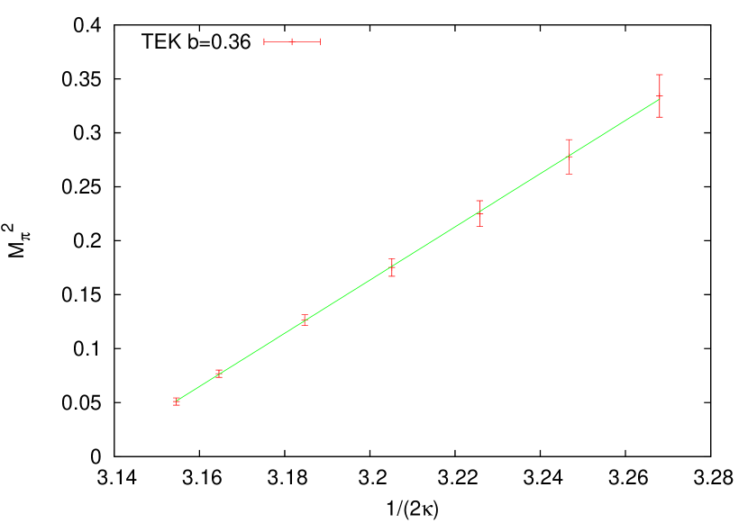
Figure 1: The pion mass square in lattice units is plotted as a function of $1/(2\kappa)$. The continuous line is a linear fit.

The pion mass follows the characteristic chiral symmetry breaking pattern, with the mass square depending linearly on $\frac{1}{2\kappa}$. This is shown in Fig. 1 for b=0.36. This allows a determination of the critical hopping parameter $\kappa_{c}$ at which the pion mass vanishes. In the case of the rho mass a linear fit of the mass works well and gives a non-zero value for the lattice mass at $\kappa=\kappa_{c}$, which we label $M_{\rho}^{(0)}(b)=m_{\rho}^{(0)}a(b)$ where $a(b)$ is the lattice spacing. For $b=0.36$ we have $\kappa_{c}=0.1596$ and $M_{\rho}^{(0)}(0.36)=0.391(3)$. For $b=0.37$ we have $\kappa_{c}=0.1559$ and $M_{\rho}^{(0)}(0.37)=0.230(3)$. The numbers at different $b$ cannot be compared without knowing the value of the lattice spacing at those $b$. In our case we can use our results for the string tension at infinite $N$ from Ref. string-tension to give the dimensionless ratio $m_{\rho}/\sqrt{\sigma}$, which comes out to be 1.90 and 1.46 for $b=0.36$ and $0.37$ respectively. This implies considerable scaling violations at these $b$ values. The errors given before are only statistical and we did not attempt a thorough estimate of the systematic errors.

It is also interesting to compare our results with those of other authors. We chose to take those of Bali et al lucini corresponding to $N=17$. Their results are obtained at $b=0.36064$, which is not far from our value of $0.36$. Nevertheless, a way to circumvent the difference in scale is to use $m_{\rho}^{(0)}$ to fix the scale. This might take away part of the systematic error. In Figs 3-3 we display $m_{\rho}/m_{\rho}^{(0)}$ as a function of $(m_{\pi}/m_{\rho}^{(0)})^{2}$. For small pion masses this quantity behaves as a straight line with intercept at 1. Our result at b=0.36 is displayed in Fig. 3 and compared with the same determination from Ref. lucini for N=17. The result is in perfect agreement. The fitted slope for our data is 0.326, and that for the values of Ref. lucini is 0.3275. The precision is somewhat accidental since a quadratic fit covering the full range of the data of Bali et al gives a slope at the origin of 0.371. Our data for b=0.37, displayed in Fig. 3, also demand a quadratic fit giving a slope at the origin of 0.351. It is clear from the figure, that errors are much larger in this case. For the purpose of this letter we are satisfied to see that our method produces very reasonable numbers with fairly limited computational resources.

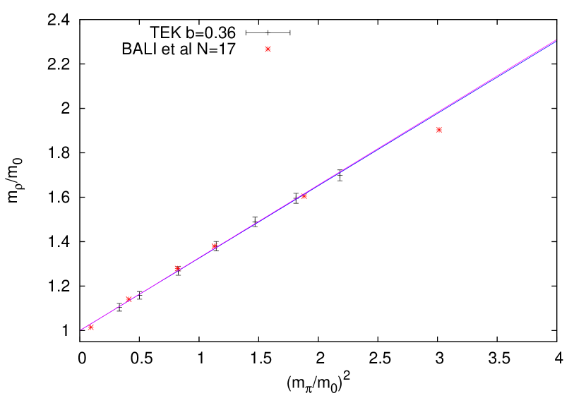
Figure 2: The $\rho$ mass versus the square of the pion mass for our $b=0.36$ data. All masses in units $m_{0}=m_{\rho}^{(0)}$. The plot also shows the data of Ref. lucini and linear fits to both sets of data.

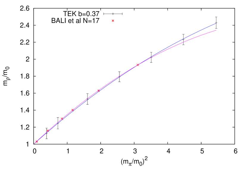
Figure 3: The same as Fig. 3 for our b=0.37 data. Fits are now given to quadratic functions.

We now summarize our conclusions. In this letter we showed how one can compute the meson masses at large $N$ using a single-site lattice model. The formula is quite simple, and using it we obtained results which are very similar to those obtained by other methods with a very limited amount of resources. In this work we opted for brevity, focusing on deriving and testing the formula for Wilson quarks in the fundamental representation in the 4-dimensional SU($N$) theory at large $N$. The idea and methodology can be readily extended to different kinds of lattice fermions, arbitrary representations of SU($N$), and different space-time dimensions. Currently we are applying the method to ‘t Hooft model in two dimensions GPGAO , in which the spectrum is known and the lattice literature is fairly scarce. Apart from testing the formula it enables to develop the technology for a precise determination in four dimensions including scalar and tensor meson masses and decay constants. There is indeed no problem in defining smeared meson operators in the reduced model okawaproc .

As mentioned earlier, the case of quarks in other representations can be addressed similarly. Despite the fact that gauge fields are defined in a one-point lattice, we should allow for quarks propagate in a larger lattice. This removes the conflict with twisted boundary conditions. Particularly interesting are the two index representations (symmetric, anti-symmetric and adjoint). However, in those cases quarks are dynamical, and the numerical task of generating thermalized configurations is much more demanding. The case of quarks in the adjoint is particularly simple since fermions can be fully reduced to a single-site GAO and dynamical quark configurations with two flavours are already available nf2 .

- (1) G. ’t Hooft, Nucl. Phys. B75, 461 (1974)
- (2) J. Erdmenger, N. Evans, I. Kirsch and E. Threlfall, Eur. Phys. J. A35, 81 (2008)
- (3) J. R. Pelaez and G. Rios, Phys. Rev. Lett. 97, 242002 (2006)
- (4) C. Bernard and M. Golterman, Phys. Rev. D46, 853 (1992)
- (5) S. R. Sharpe, Phys. Rev. D46, 3146 (1992)
- (6) L. Del Debbio, B. Lucini, A. Patella and C. Pica, JHEP 03, 062 (2008)
- (7) G. S. Bali and F. Bursa, JHEP 09, 110 (2008)
- (8) T. DeGrand, Phys. Rev. D86, 034508(2012)
- (9) G. Bali, F. Bursa, L. Castagnini, S. Collins, L. Del Debbio, B. Lucini and M. Panero, JHEP 06, 071 (2013)
- (10) A. Gonzalez-Arroyo and M. Okawa, Phys. Lett. B120, 174 (1983)
- (11) A. Gonzalez-Arroyo and M. Okawa, Phys. Rev. D 27, 2397 (1983)
- (12) A. Gonzalez-Arroyo and M. Okawa, JHEP 07, 043 (2010)
- (13) A. Gonzalez-Arroyo and M. Okawa, JHEP 12, 106 (2014)
- (14) A. Gonzalez-Arroyo and M. Okawa, Phys. Lett. B718, 1524 (2013)
- (15) M. Garcia Perez, A. Gonzalez-Arroyo, L. Keegan and M. Okawa, JHEP 01, 038 (2015)
- (16) R. Narayanan and H. Neuberger, Phys. Lett. B616, 76 (2005)
- (17) A. Hietanen, R. Narayanan, R. Patel and C. Prays, Phys. Lett. B674, 80 (2009)
- (18) R. Narayanan and H. Neuberger, Phys. Rev. Lett. 91, 081601 (2003)
- (19) A. Gonzalez-Arroyo, Advanced Summer School on Nonperturbative Quantum Filed Physics, Peniscola, Spain, 2-6 June , 57 (1997)
- (20) A. Gonzalez-Arroyo and M. Okawa, PoS(LATTICE2015) , 291 (2015)
- (21) M. Garcia Perez, A. Gonzalez-Arroyo, L. Keegan, M. Okawa and A. Ramos, JHEP 06, 193 (2015)
- (22) M. Garcia Perez, A. Gonzalez-Arroyo and M. Okawa, in preparation
- (23) A. Gonzalez-Arroyo and M. Okawa, Phys. Rev. D 88, 014514 (2013)
- (24) M. Garcia Perez, A. Gonzalez-Arroyo, L. Keegan and M. Okawa, JHEP 08, 034 (2015)