Adaptive gauge method for long-time double-null simulations of spherical black-hole spacetimes

Abstract

Double-null coordinates are highly useful in numerical simulations of dynamical spherically-symmetric black holes (BHs). However, they become problematic in long-time simulations: Along the event horizon, the truncation error grows exponentially in the outgoing Eddington null coordinate — which we denote $v_{e}$ — and runs out of control for a sufficiently long interval of $v_{e}$. This problem, if not properly addressed, would destroy the numerics both inside and outside the black hole at late times (i.e. large $v_{e}$). In this paper we explore the origin of this problem, and propose a resolution based on adaptive gauge for the ingoing null coordinate $u$. This resolves the problem outside the BH — and also inside the BH, if the latter is uncharged. However, in the case of a charged BH, an analogous large-$v_{e}$ numerical problem occurs at the inner horizon. We thus generalize our adaptive-gauge method in order to overcome the IH problem as well. This improved adaptive gauge, to which we refer as the maximal-$\sigma$ gauge, allows long-$v$ double-null numerical simulation across both the event horizon and the (outgoing) inner horizon, and up to the vicinity of the spacelike $r=0$ singularity. We conclude by presenting a few numerical results deep inside a perturbed charged BH, in the vicinity of the contracting Cauchy Horizon.

Department of Physics,

Technion - Israel Institute of Technology,

Haifa 3200003, Israel

1 Introduction

The study of perturbations of the Reissnner-Nordström (RN) background has been an area of continuing interest in black hole (BH) physics during the last few decades [1, 2, 3, 4, 5, 6, 7, 8, 9, 10, 11, 12, 13, 14]. While the perturbed Kerr geometry is considered to be a more suitable spacetime model to describe astrophysical black holes, the former model of a spherical charged BH offers a simpler analysis due to spherical symmetry. The RN and Kerr spacetimes admit a similar structure of outer and inner horizons, which implies common behavior in various phenomena; thus perturbations on RN background were often used as a “proto-type” model for BH structure both in analytical [1, 3, 5, 6, 14] and numerical [2, 7, 8, 9, 10, 11, 12, 13] analyses.

Double-null coordinates are widely used in numerical analyses of spherically symmetric spacetimes [15, 16, 17, 18, 19, 20]. The choice of double-null coordinates has several advantages: It leads to relatively simple field equations, it allows convenient coverage of globally-hyperbolic charts, and simplifies the determination of the causal structure. However, when it comes to long-time numerical simulations of (non-extremal) dynamical black-holes, it also has a serious drawback: unless preventive measures are taken, the numerical error runs out of control if the integration along the event horizon (EH) proceeds for a sufficiently long time. The time scale for the onset of this catastrophic problem, when expressed in terms of the outgoing null Eddington coordinate $v_{e}$, is typically of order $20$-$50$ times the BH mass $M$ (depending on the numerical parameters, and also on the surface gravity). The origin of this problem may be traced to dynamics at the horizon’s neighborhood, yet it destroys the numerics in the entire domain of influence of that neighborhood. This includes the BH interior (at sufficiently large $v_{e}$), and also the entire strong-field and weak-field regions at sufficiently large values of the ingoing null Eddington coordinate $u_{e}$.

To demonstrate this problem, consider two adjacent outgoing null grid rays, one just before the EH and the next one immediately after the EH. When simulation time (in $v_{e}$) is long enough, the outer ray obviously heads towards future null infinity while the inner ray heads towards either $r=0$ (e.g., in the Schwarzschild metric case) or Cauchy horizon (in the RN metric case, as illustrated in Fig. 1). This means that $\delta r$ — the difference in the area coordinate $r$ between the two adjacent grid rays at a given $v_{e}$ — grows out of control, and the numerics breaks down due to blowing-up truncation error. In fact, as long as $\delta r$ is $\ll M$, it grows exponentially with $v_{e}$ — and so is the truncation error. This exponential growth of $\delta r$ and truncation error occurs not only in that specific pair of null grid rays at the two sides of the EH, but in fact in the entire region near the horizon (both inside and outside), where $r$ is close to its value at the horizon.

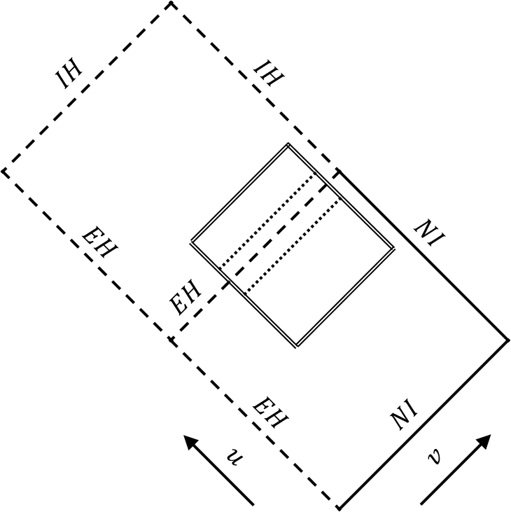
Figure 1: Spacetime diagram illustrating the resolution loss problem in a double-null numerical simulation. The diagram locates the double-null numerical grid in the RN spacetime diagram; the grid boundaries are marked by double solid lines. Solid (single) lines denote null infinity (NI); dashed lines represent the event horizon (EH) and inner horizon (IH). Dotted lines denote two adjacent grid lines, the “outer ray” and “inner ray”, at the two sides of the EH.

We have encountered this problem of uncontrolled growth of error when we attempted to numerically investigate the recently-discovered phenomenon of outgoing shock wave [21] that forms at the outgoing inner horizon of a perturbed charged (or spinning) BH. Our algorithm for overcoming this problem was developed especially for this purpose; yet we believe that this numerical algorithm may be useful for a variety of problems associated with spherical dynamical BHs. Hence the present paper will be devoted to presenting this algorithm; the results of our numerical investigation of the shock wave will be presented elsewhere.

This numerical problem has been previously addressed by Burko and Ori [9] using the so-called “point splitting” algorithm, which is based on steady addition of new grid points at the vicinity of the horizon while propagating in the $v$ direction. This algorithm is very effective, yet it is fairly cumbersome. Here we propose a different solution to that problem, based on adaptive gauge choice for the ingoing null coordinate $u$. The effect of this adaptive gauge is similar to crowding the null grid rays in the vicinity of the horizon. This solution is simpler and more versatile. It is also generalizable to similar problems that occur near the inner horizon of a charged black hole.

The paper is organized as follows: We formulate the physical problem in terms of the field equations, initial conditions, and coordinate choice in section 2; we present the basic “four-point” numerical scheme (for double-null integration of PDEs in effectively $1+1$ spacetime) in section 3. Note that sections 2 and 3 contain fairly standard material, which we nevertheless present here for the sake of completeness and for establishing our notation. The EH problem is then described in some detail in section 4; our solution for this problem, based on the adaptive-gauge method, is described in section 5. This section also contains a description of another variant of the algorithm (the “Eddington-like gauge” variant), as well as a few examples of relevant numerical results. The analogous inner-horizon problem is then discussed in section 6, and our solution to this problem — an appropriate extension of the adaptive-gauge method of section 5 — is presented in section 7. Section 8 contains a few examples of numerical results describing the behavior of the various fields deep inside the perturbed charged BH at late time (namely at large $v_{e}$, close to the contracting Cauchy horizon). We summarize our results and conclusions in section 9.

2 The physical system and field Equations

Let us consider a spherically-symmetric pulse of self-gravitating scalar field $\Phi$, which propagates inward on the background of a pre-existing Reissnner-Nordström black hole and perturbs its metric. The scalar field is neutral, massless, and minimally coupled, and the initial RN background has mass $M_{0}$ and charge $Q$. We use double-null coordinate system $(u,v,\theta,\varphi)$, and the line element is given by:

$$ds^{2}=-e^{\sigma(u,v)}dudv+r(u,v)^{2}d\Omega^{2}$$ (1)

where $d\Omega^{2}=d\theta^{2}+\sin^{2}\theta\,d\varphi^{2}$. The unknown functions in our problem are thus the scalar field $\Phi(u,v)$ and the metric functions $r(u,v)$ and $\sigma(u,v)$.

The pulse starts at a certain ingoing null ray $v=v_{1}$; hence, at $v<v_{1}$ the scalar field vanishes and the metric is just RN with mass $M_{0}$ and charge $Q$. However, at $v=v_{1}$ the metric functions are deformed by the energy-momentum contribution of the scalar field (unless the scalar field perturbation is a test field).

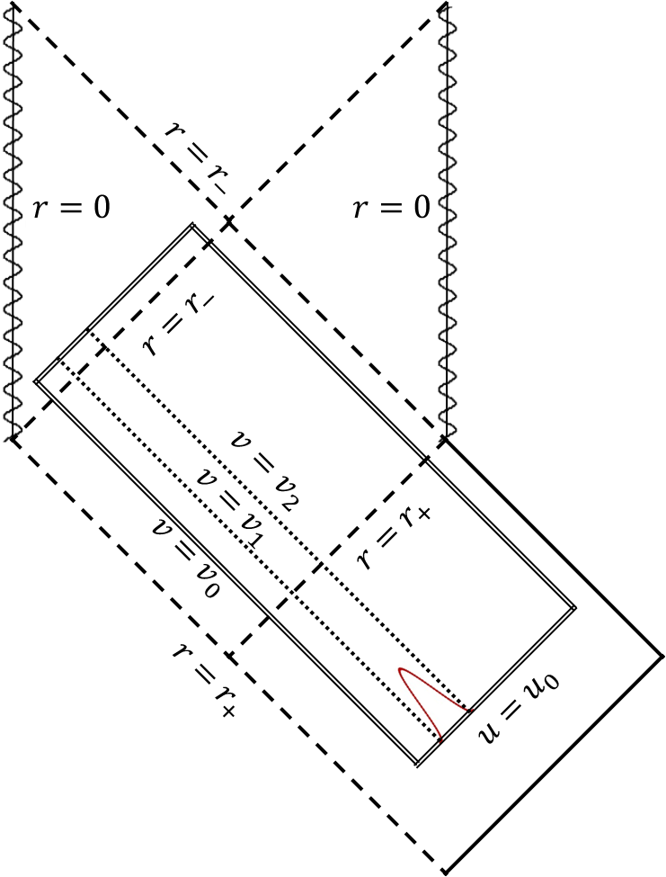
Figure 2: Spacetime diagram illustrating a typical initial-value setup for the simulation in perturbed RN spacetime. Grid boundaries are again marked by double lines. Solid lines denote null infinity; dashed lines represent the event horizon ($r=r_{+}$) and inner horizon ($r=r_{-}$). Wavy lines denote the time-like $r=0$ singularity of RN. The ingoing scalar field pulse, defined on the initial ray $u=u_{0}$, is marked by the red curve. It is initially limited to the range $v_{1}\leq v\leq v_{2}$. In the case of self-gravitating scalar field the original RN metric is deformed at $v>v_{1}$.

2.1 Field equations

The field equations and also the energy-momentum contributions of the scalar and electromagnetic fields are described in some detail in Appendix A. In our double-null coordinates the massless Klein-Gordon equation $\Phi_{;\alpha}^{\,\,;\alpha}=0$ reads

$$\Phi,_{uv}=-\frac{1}{r}(r,_{u}\Phi,_{v}+r,_{v}\Phi,_{u}).$$ (2)

The metric evolution is governed by the Einstein equation $G_{\mu\nu}=8\pi(T_{\mu\nu}^{\Phi}+T_{\mu\nu}^{Q})$, where $T_{\mu\nu}^{\Phi}$ and $T_{\mu\nu}^{Q}$ respectively denote the energy-momentum tensors of the scalar and electromagnetic fields. Substituting the explicit expressions (31,36) for $T_{\mu\nu}^{\Phi}$ and $T_{\mu\nu}^{Q}$ in the Einstein equations, one obtains two evolution equations

$$r,_{uv}=-\frac{r,_{u}r,_{v}}{r}-\frac{e^{\sigma}}{4r}(1-\frac{Q^{2}}{r^{2}}),$$ (3)

$$\sigma,_{uv}=\frac{2r,_{u}r,_{v}}{r^{2}}+\frac{e^{\sigma}}{2r^{2}}(1-\frac{2Q^{2}}{r^{2}})-2\Phi,_{u}\Phi_{,v}\,\,,$$ (4)

as well as two constraint equations

$$r,_{uu}-r,_{u}\sigma,_{u}+r(\Phi,_{u})^{2}=0,$$ (5)

$$r,_{vv}-r,_{v}\sigma,_{v}+r(\Phi,_{v})^{2}=0.$$ (6)

Overall we have a hyperbolic system of three evolution equations (2-4) for our three unknowns $\Phi(u,v)$, $r(u,v)$, and $\sigma(u,v)$. The two constraint equations need only be satisfied at the initial hypersurface (see footnote 5below).

2.2 Mass function

In addition to our three unknown functions, one may also be interested in the mass function, $m(u,v)$. The mass function is determined from the metric functions according to [5]

$$g^{\alpha\beta}r,_{\alpha}r,_{\beta}=1-2m/r+Q^{2}/r^{2},$$ (7)

which in our coordinates translates to

$$m=(1+4e^{-\sigma}r,_{u}r,_{v})r/2+Q^{2}/2r.$$ (8)

The actual numerical calculation of $m(u,v)$ is based on the numerical results of $r(u,v)$ and $\sigma(u,v)$ and finite-difference approximation for the derivatives $r,_{u},r,_{v}$.

In particular, we shall later refer to the black-hole “final mass” ($m_{final}$) which we define as the value of the mass function at the intersection of the event horizon with the final ray of the numerical grid, $v=v_{max}$.

2.3 Gauge freedom

The field equations in their double-null form (2-6) are invariant under coordinate transformations of the form $v\rightarrow v^{\prime}(v),u\rightarrow u^{\prime}(u)$. In such a transformation, obviously $r$ and $\Phi$ are unchanged, but $\sigma$ changes according to

$$\sigma\rightarrow\sigma^{\prime}=\sigma-\ln(\frac{du^{\prime}}{du})-\ln(\frac{dv^{\prime}}{dv})\,.$$ (9)

The choice of optimal gauge may depend on the nature and properties of the spacetime chart being investigated. For example, if the domain of integration is restricted to the BH exterior, an Eddington-like $u$ coordinate may be very convenient. But on the other hand if this domain contains the horizon, then one has to choose another gauge for $u$, because the Eddington-like $u$ diverges at the horizon. In that case, a compelling $u$ coordinate is the one that coincides with the affine parameter along the ingoing initial ray, to which we shall refer as an affine $u$ coordinate. (Recall, however, that in a numerical application, if the domain of integration has too large extent in $v$, then one would still run into the aforementioned “horizon problem”). In all these cases, an Eddington-like $v$ coordinate may be a reasonable choice, and the same for affine $v$ coordinate — regardless of the choice of $u$.

2.4 Characteristic initial conditions

The characteristic initial hypersurface consists of two null rays, $u=u_{0}$ and $v=v_{0}$ (see Fig. 2). In principle, the initial conditions for the hyperbolic system (2-4) should consist of the six initial functions $\Phi(u_{0},v)$, $r(u_{0},v)$, $\sigma(u_{0},v)$ and $\Phi(u,v_{0})$, $r(u,v_{0})$, $\sigma(u,v_{0})$; however, on each null ray, only two of the three functions may be freely chosen. The third function should then be dictated by the relevant constraint equation — Eq. (5) at $v=v_{0}$ and Eq. (6) at $u=u_{0}$.

In our set-up, we freely choose the two variables $\Phi$ and $\sigma$ along each initial ray, and then determine $r$ along that ray from the constraint equation. Recall, however, that there is one gauge degree of freedom associated to each initial ray. Consider for example the ray $u=u_{0}$: The initial function $\sigma(u_{0},v)$ may be modified in a fairly arbitrary manner by a gauge transformation $v\rightarrow v^{\prime}(v)$ (for example it can always be set to zero by such a transformation). Restated in other words, the choice of gauge for $v$ can be expressed by the choice of initial function $\sigma(u_{0},v)$. The same applies to the other initial ray $v=v_{0}$ and the function $\sigma(u,v_{0})$ defined along it.

We conclude that of the three initial functions that need be defined along each initial ray, one ($\sigma$) expresses the choice of gauge, one ($r$) is determined by the constraint equation, and only one ($\Phi$) expresses a true gauge-invariant physical degree of freedom.

2.4.1 The standard gauge condition

A compelling gauge choice is the one defined by the initial conditions

$$\sigma(u,v_{0})=0\,,\;\sigma(u_{0},v)=0.$$ (10)

We shall refer to it as the “standard gauge condition”. Note that this gauge condition implies an affine gauge for both $u$ and $v$.

3 The basic numerical algorithm

We solve the field equations on a discrete numerical $(u,v)$ grid, with fixed spacings $\Delta u$ and $\Delta v$ in these two directions. The borders of the grid are defined by four null rays: The two initial rays $u=u_{0}$, $v=v_{0}$ where initial data are specified, and the two final rays $u=u_{max}$, $v=v_{max}$. The numerical solution proceeds along $u=const$ lines in ascending order, from $u=u_{0}$ up to $u=u_{max}$. Along each line the solution is numerically advanced from $v=v_{0}$ up to $v=v_{max}$.

The basic building block of our algorithm, the grid cell, is portrayed in Fig. 3. It consists of three grid points (1,2,3) in which the functions $\Phi$, $r,$ and $\sigma$ are already known (from initial conditions or from previous numerical calculations), and one point (“4”) in which these functions are not known yet. The most elementary numerical task is to calculate the values of these three unknowns — which we denote by $\Phi_{4}$, $r_{4},$ $\sigma_{4}$ — at point 4 . To this end we evaluate the evolution equations (2-4) at the central point “0” (a fiducial point not included in the numerical grid), using central finite differences at second-order accuracy.

To demonstrate the basic numerical algorithm let us use the generic symbol $x$ to represent the three unknowns $\Phi$, $r,$ $\sigma$. The evolution equation for $x$ takes the schematic form

$$x,_{uv}=F(x,x_{,u},x_{,v})$$ (11)

(with some given function $F$). We evaluate this equation at point 0:

$$x,_{uv\,0}=F(x_{0},x_{,u\,0},x_{,v\,0})\equiv F_{0}\,,$$ (12)

where $x_{0}$ stands for $x$ evaluated at point 0 (and similarly for $x,_{u\,0}$, $x,_{v\,0}$, $x,_{uv\,0}$). For $x,_{uv\,0}$ we have, at second-order accuracy,

$$x,_{uv\,0}\cong\frac{x_{4}-x_{3}-x_{2}+x_{1}}{\Delta u\Delta v}\,,$$ (13)

where $x_{i}$ denotes the value of $x$ at point $i$. Next we turn to evaluate $F_{0}$. For $x_{0}$ we can simply write $x_{0}=(x_{2}+x_{3})/2$. For $x_{,u\,0}$ and $x_{,v\,0}$, the correct expressions (at second-order accuracy) would be

$$x_{,u\,0}\cong\frac{x_{3}-x_{1}+x_{4}-x_{2}}{2\Delta u}\>,\quad\quad x_{,v\,0}\cong\frac{x_{2}-x_{1}+x_{4}-x_{3}}{2\Delta v}\,.$$ (14)

Substituting these expressions for $x_{0}$, $x,_{u\,0}$, $x,_{v\,0}$ and $x,_{uv\,0}$ in Eq. (12) would yield an algebraic equation (assuming an algebraic function $F$) for the unknown $x_{4}$. In order to avoid non-linear algebraic equations, we apply a predictor corrector scheme:

• In the first stage (“predictor”), the first-order derivatives at the R.H.S. of Eq. (12) are evaluated at first-order accuracy only, through the expressions $x_{,u\,0}\approx\frac{x_{3}-x_{1}}{\Delta u}$ and $x_{,v\,0}\approx\frac{x_{2}-x_{1}}{\Delta u}$, hence $F_{0}$ is independent of $x_{4}$. Therefore, at the predictor stage Eq. (12) yields a linear equation for $x_{4}$. We mark the solution of this linear equation by $\tilde{x}_{4}$. This intermediate value $\tilde{x}_{4}$ is only first-order accurate.

• In the second stage (“corrector”), we elevate the expression for $x_{4}$ from first-order to second-order accuracy. To this end, we use the above expressions (14) for $x,_{u\,0}$ and $x,_{v\,0}$ but with $x_{4}$ replaced by $\tilde{x_{4}}$ (a known quantity). Again, $F_{0}$ is independent of the unknown $x_{4}$, and we obtain a linear equation for this unknown — which is now second-order accurate.

When applying this procedure to our actual variables, we find it convenient to solve the three evolution equations in a specific order: We first solve Eq. (3) to obtain $r_{4}$, then Eq. (2) for $\Phi_{4}$, and finally Eq. (4) for $\sigma_{4}$. This way, the predictor-corrector is not needed in the integration of the last equation (4) (as can be easily verified from its R.H.S.). We also find it convenient to choose equal grid spacings, $\Delta u=\Delta v\equiv\frac{M_{0}}{N}$, where $M_{0}$ is the initial black hole mass and $N$ takes several values $40,80,160,320,640$ (several values are used on each run to provide numerical convergence indicators).

This basic numerical scheme usually performs very well — second order convergence of $r,\sigma$ and $\Phi$ — as long as the domain of integration is not too large (say, a span in $v_{e}$ smaller than $20$ times $M$). Even if the domain of integration is much larger, the scheme should still function well if this domain is entirely outside the BH. But if the domain of integration contains a sufficiently long portion of the EH, the numerical scheme encounters the aforementioned “horizon problem”, which we now explore.

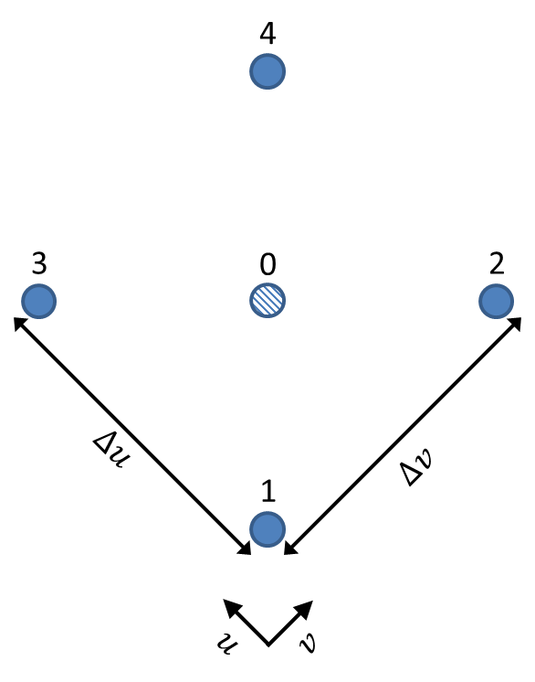
Figure 3: The basic grid cell. Points 1-4 are grid points; point 0 is an auxiliary point in which the field equations are evaluated using finite differences. The distances between adjacent grid points in the $u,v$ directions are $\Delta u$ and $\Delta v$ respectively.

4 The event-horizon problem

4.1 Simplest example: test scalar field

To illustrate the EH problem in its simplest form, suppose for example that we want to numerically analyze the evolution of a test scalar field $\Phi$ on a prescribed RN (or possibly Schwarzschild) background. Let $U_{k}$, $V_{k}$ be the Kruskal coordinates, and, recall, $u_{e}$, $v_{e}$ denote the Eddington coordinates (e.g. of the BH exterior). Suppose that our numerical chart contains (parts of) the BH exterior as well as interior, so it also contains a portion of the EH. Then certainly we cannot use the coordinate $u_{e}$ to cover this chart, because it diverges at the horizon. Instead, we can in principle use $U_{k}$, or any other $u$-coordinate regular at the horizon (e.g. the “affine $u$ coordinate” introduced in Sec. 2.3) . For the $v$ coordinate the issue of regularity at the EH does not arise at all, and we can choose $V_{k}$ or $v_{e}$ (or essentially any other $v$ coordinate), it doesn’t really matter; Nevertheless it turns out that the EH-problem is easiest to describe and quantify in terms of the $v_{e}$ coordinate, so we shall use this coordinate here.

Once we choose a horizon-regular $u$ coordinate (and essentially any $v$ coordinate), both the metric and the scalar field $\Phi$ are perfectly regular across the horizon. This is indeed the situation from the pure mathematical view-point. However, in a numerical implementation the situation becomes more problematic. It turns out that along the horizon’s neighborhood the truncation error grows exponentially in $v_{e}$. In the Schwarzschild case it grows as $\propto e^{v_{e}/4M}$, and in the more general case as $\propto e^{\kappa_{+}v_{e}}$, where $\kappa_{+}$ is the surface gravity of the EH. There is a pre-factor which is proportional to the basic spacing $\Delta u$, but if the $v_{e}$-extent of the numerical chart is sufficiently large, the exponentially-growing error eventually gets too large values and the numerics actually breaks down.

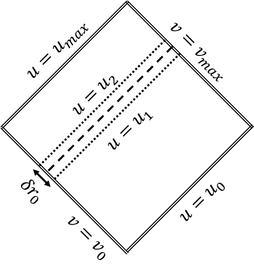
Figure 4: A zoom on the numerical grid of Figure 1 illustrating the resolution loss problem. Double solid lines denote the grid past ($u=u_{0},v=v_{0}$) and future ($u=u_{max},v=v_{max}$) boundaries. The dashed line is the EH. The dotted lines denote two adjacent null grid lines close to the event horizon, $u=u_{1}$ and $u=u_{2}$. The arrow represents the initial radial difference $\delta r_{0}$.

To understand and quantify this exponential growth of error, consider two adjacent outgoing null grid lines, denoted $u=u_{1}$ and $u=u_{2}$ (with $u_{2}=u_{1}+\Delta u$): $u_{1}$ is the last $u=const$ grid line before the EH and $u_{2}$ is the next one, as illustrated in Fig. 4. At any $v=const$ line, we denote by $\delta r(v)$ the $r$-difference between these two $u$ values:

$$\delta r(v)\equiv r(u_{1},v)-r(u_{2},v).$$

To evaluate $\delta r(v)$ we shall employ the tortoise coordinate $r_{*}(r)$ which is defined, both inside and outside the EH, as

$$r_{*}=r+\frac{r_{+}^{2}}{r_{+}-r_{-}}\ln|r-r_{+}|-\frac{r_{-}^{2}}{r_{+}-r_{-}}\ln|r-r_{-}|\,.$$ (15)

This function is non-invertible, but we can use the near-horizon approximation for $r(r_{*})$:

$$r\cong r_{+}\pm C_{\pm}e^{2\kappa_{+}r_{*}},$$

where the “$\pm"$ refers to points outside or inside the EH, and $C_{\pm}>0$ are certain constants whose specific values are unimportant here. Thus, denoting by $r_{1},r_{2}$ the values of $r$ along the lines $u=u_{1},u=u_{2}$ respectively (at a given $v$), we write

$$r_{1}\cong r_{+}+C_{+}\cdot e^{2\kappa_{+}r_{*}},\,\,\,r_{2}\cong r_{+}-C_{-}\cdot e^{2\kappa_{+}r_{*}}.$$

Let us now re-express $r_{1,2}$ using Eddington coordinates $v_{e},u_{e}$, defined (at the two sides of the EH) by $v_{e}=t+r_{*}$ and $u_{e}=\pm(t-r_{*})$, implying $r_{*}=(v_{e}\mp u_{e})/2$. [Note that regardless of the specific gauge that we actually use for $u$ in the numerics, we are allowed to re-express $u$ in terms of $u_{e}$, which simplifies the analysis here; and the same for $v_{e}$.] We find that

$$\delta r(v)\equiv r_{1}(v)-r_{2}(v)\cong e^{\kappa_{+}v_{e}}\left[C_{+}e^{-\kappa_{+}u_{e1}}+C_{-}e^{+\kappa_{+}u_{e2}}\right]\,,$$ (16)

where $u_{e1},u_{e2}$ are the Eddington values of $u_{1},u_{2}$. Notice that the term in squared bracket is a constant. Let us denote by $\delta r_{0}$ the initial value of $\delta r$ (at $v=v_{0})$. We find that

$$\delta r(v)\cong\delta r_{0}\,e^{\kappa_{+}(v_{e}-v_{e0})}\,,$$ (17)

where $v_{e0}$ is the Eddington value corresponding to $v=v_{0}$.

Since the field equation explicitly depends on $r$ (and its derivatives), the exponential growth of the difference in $r$ between two adjacent grid points will inevitably lead to an exponentially growing truncation error. If the span in $v_{e}$ is large enough, at some point $\delta r(v)$ will become so large (e.g. comparable to $r$ itself) that the finite-difference numerics will inevitably break down.

To demonstrate how severe this problem is, suppose for example that we want to explore the formation of power-law tails of the scalar field along the horizon of a Schwarzschild (or possibly RN) BH. A reliable description of tail formation typically requires a $v_{e}$ range of order a few hundreds $M$ (see e.g. Burko and Ori [9]). Let us denote this desired $v_{e}$ extent by $\delta v_{e}$, and pick for example $\delta v_{e}=200M$. Assuming that the exponential law (17) applies, and recalling that in Schwarzschild $\kappa_{+}=1/(4M)$, we find that $\delta r_{final}\equiv\delta r(v_{max})$ is $e^{50}\,\delta r_{0}\sim 5\cdot 10^{21}\,\delta r_{0}$. For any reasonable choice of initial $\Delta u$, in any “conventional” (horizon-crossing) gauge for $u$, such $\delta r_{final}$ will be $\gg M$, rendering the numerical finite-difference scheme useless. An equivalent assessment can be made in the RN case. However this phenomenon does not occur in the extremal case, because $\kappa_{+}$ vanishes.

Note however that the simple exponential growth of $\delta r(v)$ only holds as long as the two outgoing rays are still in the EH neighborhood. In particular, it is not valid when $\delta r(v)$ is no longer $\ll r_{+}$. Nevertheless, one can show that whenever Eq. (17) predicts (upon extrapolation) values of $\delta r(v_{max})$ that are comparable or larger than $r_{+}$, the actual $\delta r(v)$ between two adjacent rays bordering the EH will always achieve values of order $r_{+}$ at least (regardless of how small $\delta r_{0}$ was initially). Figure 5 displays $\delta r(v_{e})$ for a RN background with $Q/M\cong 0.65$, and a pair of grid lines (located in both sides of the EH) with initial separation $\delta r_{0}=10^{-3}M$. The figure was generated using the analytical relation between $r_{*}$ and $r$ in RN, Eq. (15).

So far we restricted the discussion to a pair of adjacent grid lines $u=u_{1,2}$ at the two sides of the EH. It is straightforward to show, however, that basically the same phenomenon occurs when the pair $u_{1},u_{2}$ in consideration is located either outside or inside the EH (but near the horizon). In all three cases $\delta r$ admits the same exponential growth (17). Note that in the case of two inner grid lines in RN the final separation $\delta r_{final}$ may be fine for large $\delta v_{e}$, because both inner rays runs to $r=r_{-}$; Yet the numerics still breaks down because in intermediate $v$ values $\delta r(v)$ becomes $\sim M$.

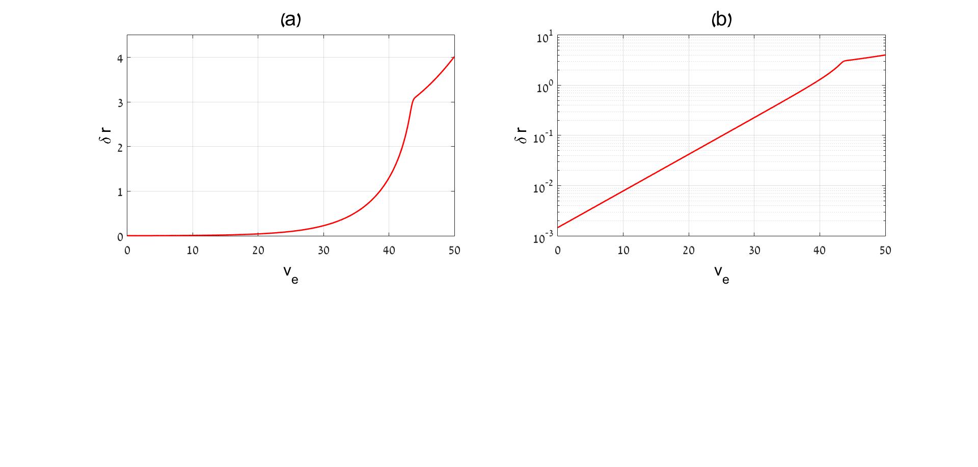
Figure 5: The event horizon problem as demonstrated from analytical results for the RN spacetime. We consider here the specific example of mass parameter $M=1.4587$ and charge parameter $Q=0.95$ in which $Q/M\simeq 0.65$, $r_{+}\simeq 2.565$, $r_{-}\simeq 0.352$ and $\kappa_{+}\simeq 0.168$. The red line represents the actual $\delta r(v_{e})$ for two adjacent grid lines in different sides of the horizon, characterized by $r(u_{1},v_{0})=r_{+}+5\times 10^{-4}M$ and $r(u_{2},v_{0})=r_{+}-5\times 10^{-4}M$. Panel (a) displays $\delta r$ in linear scale, and panel (b) in a logarithmic one. One can see that $\delta r(v_{e})$ has a long phase of exponential growth, and eventually it reaches a final value which is larger than $r_{+}$. The breaking point at $v_{e}\sim 44$ represents the point in which the inner line approaches the vicinity of $r=r_{-}$.

So far we considered the numerical solution of the scalar wave equation on a prescribed RN metric. Let us now address a slightly different problem: The simulations of the Einstein equations themselves, for the unknowns $r(u,v)$ and $\sigma(u,v)$, with no self-gravitating scalar field (and with or without a test scalar field). This numerical simulation should of course yield the RN geometry, and hence the aforementioned “horizon problem”, and the consequent numerics break-down, should occur in this case too.

This problem is demonstrated in panel (a) in Fig. 6, which displays the results of the numerical simulation of the Einstein equations for RN (with no scalar field), using the standard gauge condition (10). The BH parameters are $M=1$ and $Q=0.95$. The figure displays levels of $r$ as a function of $v$ and $u$. The diagonally-dashed rectangular region represents the domain where no numerical results were produced at all, due to numerics break-down. The “bottom” boundary of this dashed region is an outgoing $u=const$ ray, which starts at $r\approx r_{+}$ and runs far into the weak-field region (approaching $r\sim 60$ at $v_{max}=200$). Notice that this domain of faulty numerics also contains the entire large-$v$ (say $v>60$) portion of the BH interior.

For comparison, and in order to demonstrate that this “missing rectangle” is a mere numerical problem, panel (b) of Fig. 6 displays $r(u,v)$ for exactly the same initial data, presented using the same gauge for $u,v$ as in panel (a). The only difference is that this time, for the numerical integration a more sophisticated $u$-gauge was used (the “maximal-$\sigma$ gauge” described in Sec. 7 below, which solves the horizon problem). After numerical integration, the data were converted back to affine $u$ for presentation, to allow comparison with sub-figure (a). Thus, as long as the numerics works properly, the numerical results for $r(u,v)$ in the two panels are identical. The obvious difference is of course the missing diagonally-dashed region in the sub-figure (a), which demonstrates the catastrophic numerical horizon problem.

Figure 6: Demonstration of the event-horizon problem in the case of RN spacetime (with no scalar field). The figure displays $r(u,v)$ as obtained from the numerical simulation. In this example the BH mass parameters are $M_{0}=1$ and $Q=0.95$, which yield horizon radii of $r_{+}\simeq 1.312$ and $r_{-}\simeq 0.688$. (The initial value of $r$ is $r(0,0)=5$). Panel (a) displays the numerical results obtained using the standard gauge condition (10). The event-horizon problem expresses itself by the diagonally-striped patch, the rectangular region at the upper right, where no numerical data were produced at all. Notice that this region extends also outside the BH, up to $r\sim 60$ in this domain. For comparison, panel (b) displays $r(u,v)$ for exactly the same initial data, which were numerically produced using a method designed to resolve the event-horizon problem (the “maximal-$\sigma$ gauge” described in Sec. 7). The results in panel (b) were converted to the same gauge (10) as in panel (a) for presentation, in order to allow the comparison. Both panels are based on numerics with the same resolution $N=640$. The missing rectangle in panel (a) [unlike panel (b)] demonstrates the event-horizon problem.

4.2 Self-gravitating scalar field

Of course, the problem described above will also occur with self-gravitating scalar field, if double-null coordinates are used (with a “conventional” gauge for $u$). Due to the mechanism described above, $\delta r(v)$ will grow exponentially in $v_{e}$ along the EH. Since all three evolution equations (2,3,4) explicitly depend on $r$, the uncontrolled growth of $\delta r(v)$ will ruin the numerical evolution of all three unknowns. This catastrophic numerical problem is demonstrated in Fig. 7. The initial conditions are the same as in Fig. 6 above, the only difference is that this time there is a self-gravitating scalar field. We use here (like in Fig. 6) initial mass $M_{0}=1$ and charge $Q=0.95$, and employ the standard gauge condition (10). We send in an ingoing pulse of scalar field, prescribed along the initial ray $u=u_{0}$ by

$$\Phi(u_{0},v)=\begin{cases}\begin{array}[]{c}A\,\frac{64(v-v_{1})^{3}(v_{2}-v)^{3}}{(v_{2}-v_{1})^{6}}\\ 0\end{array}&\begin{array}[]{c}|\,v_{1}\leq v\leq v_{2}\\ |\,\,\,\,\,otherwise\end{array}\end{cases}$$ (18)

with $A=0.115$. This function increases smoothly and monotonically from zero (at $v=v_{1}$) to a maximum of height $A$ (at $v=\frac{v_{1}+v_{2}}{2}$), and then decreases smoothly and monotonically back to zero (at $v=v_{2}$). Throughout this paper, the scalar field vanishes on the initial ray $u=u_{0}$ – $\Phi(u,v_{0})=0$. In this case, too, one can see in panel (a) that the entire large-$v$ portion of the BH interior is missing (and also a piece of the strong- and weak-field regions outside the BH). Panel (b) presents the numerical solution with exactly the same initial data, and displayed using the same gauge for $u,v$ as in the left panel — a numerical solution produced using the “maximal-$\sigma$ gauge” for $u$ (developed later in Sec. 7). It again demonstrates that the missing diagonally-dashed region in panel (a) is a mere numerical artifact.

One can notice a missing region in panel (b) as well — the criss-crossed region at $u>10$. However, this missing region is not a numerical artifact: It results from the fact that the evolution with self-gravitating scalar field terminates at a spacelike $r=0$ singularity (unlike in the test-field case).

Figure 7: Demonstration of the event-horizon problem in the case of a spherical charged BH perturbed by self-gravitating scalar field. Apart from the difference in the physical case, this figure is similar to figure 6. The BH in this example has final mass $m_{final}\approx 1.4587$ (while $M_{0}=1$) and charge parameter $Q=0.95$, which yield horizon radii of $r_{+}\simeq 2.565$ and $r_{-}\simeq 0.352$. The event horizon problem is evident in panel (a) as a “hole” in the grid (the diagonally striped patch). Again, the problematic domain extends outside the BH to $r\gg M$. Panel (b) displays results obtained with the “maximal-$\sigma$ gauge” and then converted back to the affine gauge for presentation, to allow comparison with panel (a). The numerically-covered area in panel (b) ends around affine $u$ value of $u\sim 10$ due to the encounter of the ray $v=v_{max}=200$ with the close neighborhood of the space-like $r=0$ singularity; the area in which numerical results are unavailable due to closeness to the singularity is marked as a criss-cross patch.

We point out that if the BH is extremal (or asymptotically extremal, or even almost extremal) this problem does not arise, because $\kappa_{+}$ vanishes in the extremal case (for numerical example, see [13]) . We shall be concerned here with non-extremal BHs. Note also that if one’s only goal was to numerically analyze a test field outside the event horizon of a prescribed BH spacetime, then this problem could be easily circumvented, by just choosing the Eddington coordinate $u_{e}$. In our case, however, we wish to explore exterior as well interior regions of the BH; And more crucially, we have a self-gravitating rather than test field, hence the metric evolves dynamically. In particular, the location of the EH is not known in advance, which would hamper attempts to tailor an effectively-Eddington $u$ coordinate to the EH.

This EH problem restricted the domain of integration in previous double-null numerical simulations of dynamical BHs, in spherically-symmetric four-dimensional models [7, 8, 9, 11] as well as in two-dimensional models [22, 23, 24]. For example, $\delta v_{e}$ was restricted to $\sim 20M$ in [8]; In two-dimensional simulations, $\kappa_{+}\,\delta v_{e}$ was restricted to $\sim 20$ in [23] and to $\sim 32$ in [24].

In some spherically-symmetric simulations of self-gravitating scalar field, coordinates other than double-null were used for specifying the components of the metric, but still, the numerical coordinates—which determine the numerical grid points—were double-null. That was the situation for example in Refs. [8] and [11], which used a kind of ingoing-Eddington coordinates but with double-null numerical grid. The problem of exponentially-growing numerical error along the horizon is encountered in this situation too, for exactly the same reason: The $r$-difference between two adjacent outgoing grid lines grows exponentially in $v_{e}$.

Burko and Ori [9] developed an algorithm to address this EH problem, using a variant of adaptive mesh. More specifically, at certain lines of constant $v$ (separated from each other by some fixed interval of $v_{e}$), some of the grid points “split” into two: Namely, new grid points are born in the neighborhood of the EH. This procedure was used in Ref. [10] for investigating the internal structure of a charged BH perturbed by self-gravitating scalar field; Similar procedures of adaptive mesh were applied to the EH problem by other authors [25, 26, 27]. This procedure works very efficiently. However, it is not obvious if this algorithm would successfully deal with the outgoing shock wave [21] that develops at the inner horizon of a perturbed charged BH. (To the best of our knowledge, this issue was not tested yet.) Besides, the numerical code implementing this “point-splitting” algorithm is fairly complicated, due to the appearance of new grid points at certain $v$ values. In particular it requires interpolations at these new-born points, to determine the values of the unknown functions there. These interpolations not only complicate the algorithm but also introduce some random numerical noise at each such event of “point splitting”. Our goal in this paper is to propose a simpler method for handling this EH problem, which will not require point-splitting—and which will successfully resolve the shock at the inner horizon as well. To this end, in the next sections we shall develop a kind of “adaptive gauge” for the $u$ coordinate, instead of adaptive mesh.

5 Horizon-resolving gauge

In a conventional gauge set-up, one usually picks the function $\sigma_{u}(u)\equiv\sigma(u,v_{0})$ along the initial ray $v=v_{0}$. A particularly simple and convenient choice is $\sigma_{u}(u)=0$ (the affine $u$ gauge), but any other choice of this function is allowed. The choice of $\sigma_{u}(u)$ completely fixes the gauge of $u$. However, this conventional strategy of gauge choice leads to the EH problem described above.

To overcome this problem, we use a different strategy for gauge fixing: We prescribe the function $\sigma(u)$ along the final ingoing ray, $v=v_{max}$. Namely, we define $\sigma_{final}(u)\equiv\sigma(u,v_{max})$. Choosing different functions $\sigma_{final}(u)$ lead to different variants of the method. Unless specified otherwise, we shall use here the simple gauge condition

$$\sigma_{final}(u)=0,$$ (19)

to which we shall refer as the “Kruskal-like” final gauge. (Another variant of the method, the “Eddington-like” final gauge, is described below).

The gauge of $v$ is selected in the more conventional form, via the initial function $\sigma_{v}(v)\equiv\sigma(u_{0},v)$, as described in more detail below.

The gauge condition (19) resolves the aforementioned horizon problem. This is demonstrated in Fig. 8 for the RN case, and in Fig. 9 for the self-gravitating scalar field case. In both figures, panel (a) displays $r(u,v)$ obtained using the horizon-resolving gauge (19). For comparison, panel (b) displays the numerical solution (with exactly the same initial conditions) produced by the original affine gauge and subsequently converted to the horizon-resolving gauge for presentation. As long as the two numerical simulations function properly, they should yield the same level curves for $r(u,v)$. Again, the diagonally-dashed region marks a domain of faulty numerics, where no numerical data were produced. Panel (b) exhibits the EH problem, the termination of the numerical solution at the EH, at $u\sim 45$. Panel (a) clearly demonstrates that the horizon-resolving gauge overcomes this problem. This is the situation in both the RN and scalar-field cases. (Notice, however, that in both these figures there is a narrow diagonally-dashed strip at the upper part of panel (a) as well. This strip indicates a failure of the horizon-resolving gauge (19) somewhere inside the charged BH. We shall return to this issue at the end of this section.)

Figure 8: Resolution of the event-horizon problem in the RN case (no scalar field). Both panels display the numerically produced function $r(u,v)$ for pure RN initial data. The BH parameters in this figure are identical to those specified in Fig. 6. In panel (a) the numerics used the horizon-resolving gauge (19). In panel (b) the numerics was based on the affine $u$ gauge, although the results are displayed in the horizon-resolving gauge to allow the comparison with (a). The diagonally striped patches in both panels represent domains in which numerical results are unavailable due to the break-down of the numerics. The figure makes it clear that the horizon-resolving gauge indeed allows large-$v$ numerical resolution of the EH (unlike the affine $u$ gauge). In particular, the entire domain of dependence outside the BH is resolved, as well as a portion of the BH interior. [The narrow diagonally-striped band at the top of panel (a) indicates the inner-horizon problem, discussed below. The horizontally striped patch in panel (b) represents a region in which the affine $u$ gauge functions well but representation of results in the EH resolving gauge is problematic due to the “freeze” of $r(u,v=0)$.]

Figure 9: Resolution of the event-horizon problem in the case of a spherical charged BH perturbed by self-gravitating scalar field. It is fully analogous to Fig. 8, except the presence of self-gravitating scalar field. The BH parameters in this figure are identical to those specified in Fig. 7. In this case too, panel (a) demonstrates the efficient resolution of the EH problem (but also the occurrence of the IH problem deeper inside the BH, as indicated by the narrow diagonally-striped band at the top).

To understand how the EH problem is resolved by the gauge condition (19), consider again $\delta r(v)$, the ($v$-dependent) difference in $r$ between two adjacent grid lines $u=u_{1}$ and $u=u_{2}$ at the horizon’s neighborhood. We already saw in the previous section that near the EH $\delta r(v)\propto e^{\kappa_{+}v_{e}}$. This now implies that $\delta r(v)$ is everywhere smaller than $\delta r(v_{max})$ (because $v_{e}(v)$ is monotonically increasing). Thus, as long as $\delta r(v_{max})$ is reasonably small, the horizon problem is solved. Restated in simple words, in our new gauge set-up $\delta r(v)$ becomes “exponentially small” rather than “exponentially large” at a typical near-horizon point (e.g. at the middle of the horizon’s section included in the numerical domain).

To estimate $\delta r(v_{max})$ we express it as $\Delta u$ times $r_{,u}^{h}$, where $r_{,u}^{h}$ denotes the value of $r_{,u}$ at the intersection point of $v=v_{max}$ and the horizon. The parameter $\Delta u$ (the numerical spacing parameter) is presumably taken to be $\ll M$, so it is sufficient to show that $r_{,u}^{h}$ is of order unity. To this end we consider the constraint equation (5) imposed along the ray $v=v_{max}$, which now reads $r,_{uu}=-r(\Phi,_{u})^{2}$. To simplify the discussion let us assume that at $v=v_{max}$ the scalar field is so diluted that it has a negligible contribution in that constraint equation. We thus get $r,_{uu}\approx 0$, meaning that $r_{,u}$ is approximately conserved along the ray $v=v_{max}$. Let $r_{,u}^{0}$ denote the value of $r_{,u}$ at point ($u=u_{0},v=v_{max}$), namely at the far edge of the outgoing initial ray. All we need is to make sure that $r_{,u}^{0}$ is of order unity (or smaller). It turns out that this parameter depends on the $v$-gauge as well; and in the way we choose our $v$-gauge (by imposing $\sigma(v)=0$ along $u=0$) $r_{,u}^{0}$ indeed turns out to be of order unity. Hence from the constraint equation $r_{,u}^{h}$ is of order unity too, which in turn ensures that $\delta r(v_{max})\ll M$, and the same for $\delta r(v<v_{max})$.

5.1 Numerical implementation: Initial-value set-up

5.1.1 Initial data at $v=v_{0}$

From the basic mathematical view-point, the characteristic initial data required for the hyperbolic system of evolution equations consist of the values of the three unknowns ($\Phi,r,\sigma$) along the two initial null rays. We focus here on the data specification along the ingoing ray $v=v_{0}$ (the initial-data set-up at the other ray $u=u_{0}$ is more conventional, and we shall briefly address it below). We denote the three initial-value functions at $v=v_{0}$ by $\Phi_{u}(u)$, $r_{u}(u)$, and $\sigma_{u}(u)$. The first two functions $\Phi_{u}(u)$, $r_{u}(u)$ can be chosen as usual: Namely, $\Phi_{u}(u)$ can be chosen at will, and $r_{u}(u)$ should be determined by the constraint equation (5). But the remaining function $\sigma_{u}(u)$ must be chosen in a special manner in order to achieve the desired gauge condition $\sigma_{final}(u)=0$. We now explain how we choose the appropriate initial function $\sigma_{u}(u)$.

We numerically integrate the PDE system along lines of constant $u$, as described in section 3 above. Suppose that we already integrated the PDE system up to (and including) a certain grid line $u=const=u_{a}$, and we turn to solve the next line, $u=u_{a}+\Delta u\equiv u_{b}$. To this end we need to specify the three initial values for this line, namely $\Phi_{u}(u_{b})$, $r_{u}(u_{b})$, and $\sigma_{u}(u_{b})$. We set $\Phi_{u}(u_{b})$ by just substituting $u=u_{b}$ in the prescribed initial function $\Phi_{u}(u)$. Then $r_{u}(u_{b})$ is to be obtained from the constraint equation (upon integration from $u_{a}$ to $u_{b}$). The more tricky task is the determination of $\sigma_{u}(u_{b})$. In principle one can do this by trial and error: For each choice of $\sigma_{u}(u_{b})$, one can integrate the PDE system along $u=u_{b}$ up to $v_{max}$ and obtain $\sigma_{final}(u_{b})$. Then one can correct $\sigma_{u}(u_{b})$ in an attempt to get a value of $\sigma_{final}(u_{b})$ closer to the desired value $\sigma_{final}(u_{b})=0$, and so on. This may be implemented by a simple iterative process, e.g. using Newton-Raphson method, which converges very rapidly. However, there is another method which turns out to be much more efficient in terms of computation time: One can find the desired value of $\sigma_{u}(u_{b})$ by extrapolation, based on the values of $\sigma_{u}(u)$ at $u=u_{a}$ and a few additional preceding $u=const$ lines (namely $u=u_{a}-\Delta u$, $u=u_{a}-2\Delta u$, … $,u=u_{a}-n\Delta u$). The number of such preceding $\sigma_{u}(u)$ values to be used in the process, would depend on the desired order of extrapolation. With this procedure, we only need to solve the evolution equations once along any $u=const$ grid line — just like in the case of the conventional gauge choice, in which $\sigma_{u}(u)$ is prescribed.

This procedure works very efficiently. By including a sufficient number of $u$-grid points in the extrapolation (that is, a sufficiently large $n$), the mismatch in $\sigma_{final}$ — namely the deviation of the latter from zero — can easily be made third order or even higher-order in $\Delta u$. In our numerical code we actually use interpolation order $n=2$. $\sigma_{final}$ is then third-order in $\Delta u$, and it is typically of order $10^{-8}$ or even smaller. One should also bear in mind that even this tiny deviation of $\sigma_{final}$ from zero does not necessarily represent an error in the numerical solution: It merely represents a deviation from the intended gauge condition $\sigma_{final}=0$ (a deviation which has no effect whatsoever on the capability of this gauge to achieve its goal of horizon-resolution).

As already mentioned above, the initial parameter $r_{u}(u_{b})$ is to be determined by integrating the constraint equation (5) from $u_{a}$ to $u_{b}$. The discretization of this ODE may involve also $\sigma_{u}(u_{b})$. But this does not pose any difficulty, because one can proceed as follows: First obtain $\sigma_{u}(u_{b})$ by extrapolation, and then determine $r_{u}(u_{b})$ from the constraint equation.

5.1.2 Initial data at $u=u_{0}$

The initial data along the outgoing ray $u=u_{0}$ are imposed in a rather conventional manner. We denote the three initial functions that need be specified along that ray by $\Phi_{v}(v)$, $r_{v}(v)$, and $\sigma_{v}(v)$. These three functions must satisfy the constraint equation (6). Our view-point concerning the role of these three initial functions is as described in section 2.3: $\Phi_{v}(v)$ is selected at will, representing the ingoing scalar pulse; $\sigma_{v}(v)$ may also be selected at will, but it merely represents one’s choice of $v$-gauge; The last function $r_{v}(v)$ is in turn determined by the constraint equation (6) — apart from its initial data, namely the values of $r$ and $r_{,v}$ at the vertex ($u_{0},v_{0}$).

The choice of $\sigma_{v}(v)$ is subject to one obvious constraint: It must coincide with the aforementioned final $u$-gauge condition; that is, $\sigma_{v}(v_{max})=\sigma_{final}(u_{0})$. In our numerical code we implemented the simplest choice $\sigma_{v}(v)=0$. Consistency at the vertex is guaranteed, by virtue of our $u$-gauge condition $\sigma_{final}(u)=0$.

To summarize, our gauge condition — throughout the external world as well as for horizon crossing — is

$$\sigma_{final}(u)=0\,,\>\sigma_{v}(v)=0\,.$$ (20)

5.2 The Eddington-like variant

In some applications one may be interested in time-dependent, dynamically evolving, BHs, but only in their external part, up to the EH — and not beyond. This is the situation, for example, when exploring the influence of the BH dynamics on the scattering of various fields/modes. A particular example is the issue of how BH dynamics affects the late-time tails of various modes, e.g. at $r=const$, at future null infinity, or along the horizon. [28, 29]

In such applications, there still is the need to numerically resolve the very neighborhood of the EH, but there is no reason to cross it. If the metric was prescribed — e.g. Schwarzschild or RN — the Eddington coordinate $u_{e}$ would be optimal for this task. However, we are concerned here with a-priori unknown dynamical metric. In particular, we don’t know in advance where the EH is. It would thus be helpful to have at our disposal a gauge-selection method which automatically yields a $u$ coordinate appropriate for such situations — namely an Eddington-like $u$ adapted to the dynamically-forming EH.

This goal is easily achieved within the framework of final-gauge condition for $u$, described above. All that one has to do is to replace the condition (19) by one appropriate to Eddington-like $u$. One such example is:

$$\sigma_{final}(u)=\ln\left(1-\frac{2m_{final}(u)}{r_{final}(u)}+\frac{Q^{2}}{[r_{final}(u)]^{2}}\right)$$

where $m_{final}(u)$ denotes the mass function evaluated at $v=v_{max}$, and similarly for $r_{final}(u)$. Here, however, we shall use a more convenient and pragmatic gauge condition which achieves this same goal, but without resorting to the mass function:

$$\sigma_{final}(u)=\ln[2(r_{,v})_{final}]$$ (21)

where $(r_{,v})_{final}\equiv r_{,v}(u,v_{max})$.

In principle, we could apply a similar gauge condition to the initial ray $u=u_{0}$. Nevertheless, we found it useful (due to certain technical reasons) to apply the gauge condition:

$$\sigma_{v}(v)=\ln\left(1-\frac{2m_{v}(v)}{r_{v}(v)}+\frac{Q^{2}}{[r_{v}(v)]^{2}}\right)$$ (22)

which also fits Eddington gauge in RN. However, it is not trivial that the different gauge conditions (21,22) would yield continuity of $\sigma$ at the corner ($u=u_{0},v=v_{max}$). Gauge condition (21) fixes the $u$ gauge completely and is unaffected by any change in the $v$ gauge, while gauge condition (22) keeps a residual gauge freedom (see footnote 6): it is unaffected by a gauge transformation of the form $v\rightarrow v\,b,u\rightarrow u/b$ (and does not fix either gauge independently). Therefore, we can achieve continuity at the corner by applying this gauge transformation on the initial data at $u=u_{0}$ with the appropriate choice of $b$.

To summarize, our gauge condition for the Eddington-like variant of the horizon-resolving gauge is:

$$\sigma_{final}(u)=\ln[2(r_{,v})_{final}]\,,\,\,\,\sigma_{v}(v)=\ln\left(1-\frac{2m_{v}(v)}{r_{v}(v)}+\frac{Q^{2}}{[r_{v}(v)]^{2}}\right).$$ (23)

5.3 Some numerical results for external tails

We shall refer to the gauge conditions (20) and (23) respectively as the Kruskal-like and Eddington-like variants of the final $u$-gauge. Since our main interest is the interior of a charged BH, in the next sections we shall use (and further develop) the Kruskal-like variant, the gauge condition (20). Nevertheless, we bring here some numerical results for both the Kruskal-like (Fig. 10) and the Eddington-like (Fig. 11) gauges, concerning late-time tails outside a dynamically-evolving BH. The initial conditions in these examples are essentially the same as the ones described in section 4.2, namely initial mass $M_{0}=1$ and charge $Q=0.95$, with ingoing scalar field pulse of the form (18) with $v_{1}=1$, $v_{2}=7$, and with $u_{0}=v_{0}=0$. The scalar field amplitude is again $A=0.115$. However, in order to reach deep into the late-time regime a larger $v_{max}$ was used here ($v_{max}=1000$ instead of $200$).

Figure 10: Numerical results obtained using the Kruskal-like gauge. The figure describes the late-time behavior of $\Phi$ and $r$ along the event horizon. Panel (a) displays the decay of $\Phi$ as a function of $v$. Panel (b) shows the local power of this decay, defined as $-v\Phi,_{v}/\Phi$.[9] In both panels the four resolutions overlap. The asymptotic local power is approximately $3$, in agreement with Price law[28] (see also [29]). Panel (c) displays $r$ as a function of $v$. As expected, $r$ is approximately constant along the curve, with a maximal drift of order $\sim 10^{-5}$ along a range $\Delta v=800$ (for the best resolution $N=640$). This drift is caused by truncation error.

Figure 11: Numerical results obtained using the Eddington-like gauge. The figure describes the late-time behavior of $\Phi$ and $r$ along the timelike curve $r*=0$, as functions of $t$, where $u_{e},v_{e}$ are the numerical Eddington-like coordinates introduced in section 5.2. Panel (a) presents the decay of $\Phi$ at large $t$. Panel (b) shows the local power characterizing this decay. Here again, in both panels the four resolution overlap, and the asymptotic local power is approximately $3$, in agreement with Price law. Panel (c) displays $r$ as a function of $t$ along the same curve $r*=0$. As expected, $r$ is approximately constant along the curve. However, there is a drift of order $\lesssim 10^{-3}$ for the best resolution ($N=320$) along $\Delta t=800$. The evident drift in the three best resolutions is caused by the fact that the constructed Eddington-like coordinates, as well as $r*$, fit Eddington coordinates in pure RN spacetime only asymptotically.

5.4 How well does the horizon-resolving gauge penetrate in?

The numerical results presented in the previous subsection made it clear that the horizon-resolving gauge (like its Eddington-like counterpart) functions very well outside the BH, all the way up to the EH. But how deeply can it penetrate into the BH? The narrow diagonally-dashed strips at the top of the left panels in Figs. 8 and 9 indicate numerical problems somewhere inside the BH. Figure 12 provides a more clear mapping of the regions of good and bad numerics, using a spacetime diagram with coordinates $r$ and $v$. Panel (a) describes the case of precisely-RN initial data (i.e. no scalar field), numerically evolved using either the affine or horizon-resolving gauges for $u$. The diagonally-dashed region marks the domain of successful numerics using the horizon-resolving gauge. Similarly, the vertically-dashed region marks the domain of numerical success of the original affine gauge. The orange thick dashed frame is the boundary of the maximal possible domain of integration — namely the entire domain of dependence of the characteristic initial data. We primarily focus here on the large-$v$ portion of the diagram (say $v>60$). One can again see that the original affine gauge does not get even close to the EH (the horizontal dashed purple line $r=r_{+}$). The horizon-resolving gauge, on the other hand, covers the entire external region up to the EH. Furthermore, at very large $v$, close to $v_{max}$ (say $v>180$ in this case) the numerically-covered region penetrates inside the BH and reaches $r\sim r_{-}$ at $v_{max}$. However, at smaller $v$ values the domain of numerical coverage hardly penetrates into $r<r_{+}$. The situation in the case of self-gravitating scalar field is basically similar, as seen in panel (b).

We shall refer to this numerical problem — this failure of the horizon-resolving gauge to traverse the IH (or even approach it effectively) — as the “inner-horizon problem”. We shall analyze it in the next section, and resolve it in Sec. 7 by further improving the gauge.

Figure 12: Numerical coverage of the horizon-resolving gauge in the spacetime of a spherical charged BH. The coverage of the affine $u$ gauge is also shown for comparison. Panel (a) presents the case of pure RN initial data, and panel (b) the case of self-gravitating scalar field. BH parameters of both cases are the same as in figures 6 and 7, respectively. Both panels presents the last reliable $r$ value on each $v=const$ grid ray as a function of numerical $v$ coordinate (which is common for both gauges). Numerical reliability is determined by the relative difference between the two best resolutions $(N=320$ and $N=640$), and the limit of reliability is chosen as the point in which the relative difference crosses a threshold $T$, where $T$ is either $1\%$ (dashed red and cyan curves) or $3\%$ (solid red and cyan curves). The red curves refer to the affine gauge, and the cyan curves to the horizon-resolving gauge. The thick dashed orange frame represents the maximal possible $r$ coverage on each case — namely boundary of the domain of dependence of the data. In panel (a), the pure RN case, the bottom orange curve is computed analytically, it corresponds to the $u=u_{max}$ ray which starts close to $r=0$ and runs toward $r=r_{-}$ (dashed magenta line). In panel (b), the case of self-gravitating scalar field, the bottom orange curve is absent (non-calculable) due to the lack of analytical solution. The region covered by the affine $u$ gauge is marked by a vertically striped patch; the region covered by the EH resolving gauge is marked by diagonally striped patch. The thin black trapezoid frame in both panels marks a region in which the affine $u$ gauge has non-robust error behavior. These graphs demonstrate clearly that the EH resolving gauge has superior numerical coverage at late times in which it enters the BH (while the affine $u$ gauge does not even get close to the EH).

6 The inner-horizon problem

If the black hole has no inner horizon (e.g. an uncharged spherical BH), the horizon-crossing gauge described above allows efficient numerical integration of the field equations all the way up to the neighborhood of the space-like $r=0$ singularity. However, as was just demonstrated, in the case of a charged BH new difficulties arise while approaching the inner horizon (IH). This will require us to further generalize our gauge condition for $u$.

To understand these IH-related difficulties, it would be simplest to consider again a test scalar field on a fixed RN background. Suppose that the outgoing initial ray is located outside the BH, and the ingoing initial ray crosses both the event and inner horizons, as in Fig. 2. We also assume that the outgoing initial ray is long, namely $\delta v_{e}\gg M$. Therefore the domain of integration contains long sections of both the event and inner horizons. Now consider two adjacent outgoing null grid lines, $u=u_{1}$ and $u=u_{2}$, this time in the immediate neighborhood of the IH. Again we consider the quantity $\delta r(v)\equiv r(u_{1},v)-r(u_{2},v)$. The analysis is analogous to the event-horizon case discussed above, and we again obtain

$$\delta r(v)=\delta r_{0}\cdot e^{-\kappa_{-}(v_{e}-v_{e0})}$$ (24)

where $\kappa_{-}>0$ is the inner-horizon surface gravity. Note the sign difference (in the exponent) between Eqs. (24) and (17): It actually reflects the difference between redshift (along the EH) and blue-shift (along the IH).

In the “final $u$-gauge” described in the previous section, at $v=v_{max}$ the difference $\delta r(v)$ naturally gets a reasonable value of order $\Delta u$. The problem is that this reasonable value of $\delta r$ at $v=v_{max}$ grows exponentially with decreasing $v_{e}$. At $v=v_{0}$ one gets $\delta r_{0}\approx\Delta u\,e^{\kappa_{-}\delta v_{e}}$. Such an exponentially-large $\delta r(v)$ naturally leads to a corresponding huge truncation error, and hence to break-down of the numerics.

In essence, the inner-horizon problem arises from the different signs of the exponents in Eqs. (17) and (24): The positive sign in the former motivated us to use the $\sigma(v_{max})$ “final $u$-gauge” at the EH, whereas the negative sign in the latter calls for using “initial $u$-gauge” at the IH.

Naively one might hope that a possible resolution would be to do the integration in two steps: First, integrate the initial data using the $u$-gauge $\sigma(v_{max})=0$ up to a certain outgoing line $u=const\equiv u_{middle}$ located somewhere between the event and inner horizons, and then integrate the remaining domain $u>u_{middle}$ using the more conventional gauge $\sigma(v_{0})=0$. This procedure does not work, however: one can show that there is a range of $u$ values, in between the EH and IH, in which neither of the two $u$-gauges $\sigma(v_{0})=0$ or $\sigma(v_{max})=0$ properly works (because in both gauges $r_{,u}$, and hence also $\delta r(v)$, gets exponentially-large values somewhere between $v_{0}$ and $v_{max}$).

To overcome this inner-horizon problem, in the next section we shall introduce a new $u$-gauge which solves this problem, and allows numerical resolution of both the event and inner horizons.

7 The solution: The maximal-$\sigma$ gauge

Consider the function $\sigma(v)$ along a line of constant $u$. We denote by $\sigma_{max}(u)$ the maximal value of this function in the range $v_{0}\leq v\leq v_{max}$. The value of $v$ at that point of maximal $\sigma$ is denoted $v_{\sigma max}(u)$.

We shall now impose the gauge condition

$$\sigma_{max}(u)=0$$ (25)

and refer to it as the maximal-$\sigma$ gauge. The gauge for $v$ remains as it was before,

$$\sigma_{v}(v)=0$$ (26)

Recall that the variable $\sigma$ depends on the gauge choice for both $v$ and $u$, through Eq. (9). The gauge of $v$ has already been fixed once and forever by the initial data at $u=u_{0}$. Along a given $u=const$ line, the effect of changing the gauge of $u$ would merely be to add $\ln(du/du^{\prime})=const$ to the original function $\sigma(v)$. Hence, such a change of $u$-gauge would not affect the location of the maximum point $v_{\sigma max}$ — but it would shift $\sigma_{max}(u)$ by that $const$. The specification of $\sigma_{max}(u)$ thus fixes the $u$-gauge freedom.

With this gauge condition, the inequality

$$\sigma(u,v)\leq 0$$ (27)

is satisfied in the entire domain of integration. This boundedness of $\sigma$ directly reflects on the magnitude of $r_{,u}$, and hence also on $\delta r$ and the truncation error, as we shortly explain. This solves the aforementioned numerical difficulties, and allows efficient long-$v$ numerical integration across both the event and inner horizons (as well as in the domain beyond the IH).

To understand how the bound on $\sigma$ affects the magnitude of $r_{,u}$ (and hence $\delta r$ and the truncation error), let us again consider the simple case of exact RN background. Assume at first stage that our $v$ coordinate is taken to be the Eddington coordinate $v_{e}$. Then, if $u$ were taken to be Eddington too, we would have $e^{\sigma}=2|r_{,u}|$, because in the RN metric in double-null Eddington coordinates both quantities are equal to $\left|1-2M/r+Q^{2}/r^{2}\right|$. In a general transformation $u\rightarrow u^{\prime}(u)$ both $e^{\sigma}$ and $|r_{,u}|$ are multiplied by the same factor $du/du^{\prime}$, hence $e^{\sigma}=2|r_{,u}|$ is preserved (as long as $v=v_{e}$). Transforming next from $v_{e}$ to a general $v$ coordinate, we find that

$$|r_{,u}|=\frac{1}{2}\frac{\partial v}{\partial v_{e}}\,e^{\sigma}$$ (28)

is satisfied in a general gauge for $u$ and $v$. Recall, however, that the ($v$-dependent) quantity $\partial v/\partial v_{e}$ is determined once and forever by the initial data at $u=u_{0}$; and in our set-up, this quantity turns out to be of order unity. We therefore conclude that in our maximal-$\sigma$ gauge, $|r_{,u}|$ is of order unity at most. Consequently $\delta r$ is bounded by $\sim\Delta u\ll 1$, and the truncation error is well under control.

So far we considered the case of exact RN background. In the more general case of nonlinearly-perturbed background metric Eq. (28) no longer holds. Nevertheless, in typical simulations $|r_{,u}|$ and $e^{\sigma}$ are still of same order of magnitude; hence (since $e^{\sigma}\leq 1$) the uncontrolled growth of $\delta r$, and the related problem of catastrophic truncation error, are prevented.

It may be instructive to understand the location of the maximal-$\sigma$ curve $v=v_{\sigma max}(u)$ (where in our new gauge $\sigma$ is set to zero). A detailed analysis of this curve can be done in the case of RN background. One finds that the integration range $u_{0}\leq u\leq u_{max}$ is divided into three domains: (I) Outside the BH — and also inside the BH up to a certain $u$ value which we denote $u_{a}$ — $v_{\sigma max}(u)=v_{max}$. (II) Next, in a certain transition domain $u_{a}<u<u_{b}$, $v_{0}<v_{\sigma max}(u)<v_{max}$; It smoothly moves in this domain from $v_{\sigma max}=v_{max}$ at $u=u_{a}$ to $v_{\sigma max}=v_{0}$ at $u=u_{b}$. (III) Then, at $u\geq u_{b}$, we have $v_{\sigma max}(u)=v_{0}$. Stated in other words, in domain (I) the “maximal-$\sigma$ gauge” coincides with the “horizon-resolving” gauge $\sigma(u,v_{max})=0$, in domain (III) it coincides with the more conventional $u$-gauge $\sigma(u,v_{0})=0$, and domain (II) is a smooth transition region.

In the exact RN case — and with Eddington $v$ — one finds that throughout the transition region (II), $v_{\sigma max}(u)$ is precisely the curve where $r=Q^{2}/M$. Correspondingly, $u_{a}$ is determined in that case by $r(u_{a},v_{max})=Q^{2}/M$, and $u_{b}$ by $r(u_{b},v_{0})=Q^{2}/M$. In our actual $v$-gauge (26), $r$ is still close to $\sim Q^{2}/M$ at $v=v_{\sigma max}(u)$ in region II. The same applies in the self-gravitating case.

This new gauge (25,26) provides a robust solution to the aforementioned EH and IH problems. This is demonstrated in Figs. 13 and 14, which correspond to the RN and self-gravitating field cases respectively. Both figures display the domain of numerical validity of the maximal-$\sigma$ gauge on a spacetime diagram in ($r,v$) coordinates. For comparison, the figures also display the domain of numerical validity of the two former gauges, namely the affine gauge and the “horizon-resolving” gauge. In Fig. 13 (Pure RN initial data), one sees that the maximal-$\sigma$ gauge effectively resolves the entire domain of dependence of the characteristic initial data (the dashed orange frame). In the more interesting case of self-gravitating scalar field the situation is more subtle: In this case, the “bottom” boundary of the domain of dependence is very close to the spacelike singularity at $r=0$. The singular nature of this boundary makes it very hard for the numerics to approach it. Nevertheless, the maximal-$\sigma$ gauge numerics allows reliable coverage up to $r$ values of order few times $10^{-2}$, as can be seen in panel (b) of Fig. 14.

Figure 13: Numerical coverage of the maximal-$\sigma$ gauge in the RN case. The coverage of the affine $u$ gauge and the horizon-resolving gauge is also shown for comparison. The graph presents the last reliable $r$ value on each $v=const$ grid ray as a function of numerical $v$ coordinate and is similar to panel (a) in figure 12, except that (i) here it shows coverage differences between three gauges (the affine $u$ gauge in red, the EH resolving gauge in cyan, and the maximal-$\sigma$ gauge in blue), and (ii) it represents each gauge with three sets of lines, each one for a different relative-error threshold $T$ (dotted lines - $1\%$; dashed lines - $3\%$; and solid lines - $10\%$). Again, the thick dashed orange frame represents the maximal possible $r$ coverage in this case. The graph demonstrates clearly that the maximal-$\sigma$ gauge has superior numerical coverage: Note that all three blue curves (representing the three error levels in the maximal-$\sigma$ gauge) overlap in this diagram — and they also overlap with the bottom orange curve. This indicates that the maximal-$\sigma$ gauge essentially covers the entire domain of dependence.

Figure 14: Numerical coverage of the maximal-$\sigma$ gauge in the presence of self-gravitating scalar field. The coverage of the affine $u$ gauge and the horizon-resolving gauge is also shown for comparison. The meaning of the various curves and symbols in this figure is the same as in Fig. 13, the only difference is the presence of the scalar field. This figure uses both a linear scale (a) and logarithmic scale (b) for the $r$ axis. The blue curve in panel (a) approximately overlaps with the $r=0$ line, indicating that the maximal-$\sigma$ gauge provides efficient numerical coverage up to very close to the spacelike $r=0$ singularity. (The significant deviation of the blue curve from $r=0$ at $v\lesssim 10$ does not represent a numerical problem: It is a true feature of the function $r(u_{max},v)$, which merely reflects the spacelike character of the $r=0$ singularity.) From the logarithmic scale in panel (b) one can see that the numerical coverage extends up to $r$ values of order a few times $10^{-2}$ (depending on the required accuracy).

7.1 Numerical implementation: Initial-value set-up

Our new gauge condition is given in Eqs. (25,26). The procedure of initial-value setup along $v=v_{0}$ is almost the same as the one described in section 5.1. There is one obvious difference in the setup of the initial value for $\sigma_{u}(u)$: Instead of extrapolating the quantity $\sigma_{u}(u)-\sigma_{final}(u)$ (see footnote 14), we now extrapolate $\sigma_{u}(u)-\sigma_{max}(u)$. This reflects the fact that we are now attempting to nullify $\sigma_{max}(u)$ rather than $\sigma_{final}(u)$. The initial-value setup along the ray $u=u_{0}$ is identical to the one described in section 5.1.

There remains the technical issue of evaluating $\sigma_{max}(u)$, the maximal value of $\sigma$ along each $u=const$ line (required for the extrapolation process that determines $\sigma_{u}(u)$.) The first obvious step is to find the grid point of maximal $\sigma$ along the $u=const$ line under consideration. However, this is not always sufficient. As was mentioned above, the $u_{0}\leq u\leq u_{max}$ range is divided into three domains, according to the value of $v_{\sigma max}(u)$. In domain I we have $v_{\sigma max}(u)=v_{max}$, hence $\sigma_{max}(u)$ is simply the value of $\sigma$ at the last grid point ($v=v_{max}$). Similarly in domain III, $\sigma_{max}(u)$ is the value of $\sigma$ at the first grid point ($v=v_{0}$). However, in the transition domain II the situation is slightly more complicated: In a generic $u=const$ line in this domain, $v_{\sigma max}(u)$ will be located in between two grid points. If one approximates $\sigma_{max}(u)$ by one of these two points (e.g. the one with the largest $\sigma$), this leads to a discretization noise (amplified by the extrapolation process) which may seriously damage the accuracy of our second order extrapolation. Therefore we need here a more precise evaluation of $\sigma_{max}(u)$. To this end, we carry a second-order interpolation of $\sigma(v)$ (along the $u=const$ line) in the neighborhood of the grid point of maximal $\sigma$, and determine $\sigma_{max}(u)$ from this interpolation. This procedure eliminates most of the numerical noise in the extrapolation.

8 Some numerical results deep inside the charged black hole

The maximal-$\sigma$ gauge described above enables us to efficiently prob the innermost zone $0<r\leq r_{-}$ of the perturbed charged BH, even at very late times (i.e. large $v_{e}$). As an example, we choose here to explore the behavior of $r$ and $\Phi$ along the contracting Cauchy horizon (CH) and its neighborhood, in the case of self-gravitating scalar field. All results below correspond to the same numerical simulation of a charged BH with a self-gravitating scalar field, with the same set of parameters as described in Sec. 4.2. Note that in all figures throughout this section, the numerical results were produced with two different resolutions, $N=320$ (dashed curves) and $N=640$ (solid curves), in order to control the numerical error. In almost all cases the dashed curve is visually undistinguished from the solid curve, indicating negligible numerical error. (The exceptions are panels (c) and (d) in Fig. 18, where the high zoom level in $r$ ($\lesssim 10^{-5}$) allows us to see the small differences between the resolutions).

We argue that the behavior of various quantities along the CH should be well represented by the lines $v=const$ with sufficiently large value of the “$const$”. To theoretically examine this issue let us consider the case of RN background with test scalar field. Then two separate issues are involved here: (i) In the domain beyond the (outgoing section of the) IH, all outgoing null rays run to $r=r_{-}$ at the limit $v_{e}\to\infty$. The “distance” from the IH (in terms of $r$ values) at finite $v_{e}$ scales as $e^{-\kappa_{-}v_{e}}$. (ii) Wave-scattering dynamics takes the asymptotic form $\Phi(u,v)\cong f_{u}(u)+f_{v}(v)$ near the IH, and at sufficiently large $v$ (namely $v_{e}\gg m$) we have $f(v)\propto(v_{e}/m)^{-3}$. The scalar field thus approaches the CH limiting function $\Phi\simeq f_{u}(u)$ at $v_{e}\gg m$. With $v_{max}=200$ the first issue (i) is perfectly well addressed as $e^{-\kappa_{-}\delta v_{e}}$ is extremely small. Concerning the other issue (ii), at $v=200$ wave dynamics is considerably suppressed — namely $f_{v}(v)$ is negligible to a fairly good approximation (although here the approximation is not as good as it is in regards to the first issue, because the decay here is inverse-power rather than exponential).

In the presence of self-gravitating scalar field the near-CH dynamics becomes more complicated and we shall not discuss it here. Nevertheless, the $v=const$ lines with sufficiently large “$const$” should still mimick the CH. The quality of this “CH-mimicking” approximation for large-$v$ rays will be verified by the numerical results that we shortly display.

Figure 15 displays $r(u)$ along rays of constant $v$. This figure demonstrates two interesting (although well known) facts: First, while $u$ increases the various constant-$v$ curves join a universal limiting curve (the red curve at the bottom), which should be interpreted as $r(u)$ along the CH. Second, the CH undergoes a clear contraction at large $u$: The CH function $r(u)$ is initially “frozen” at $r\approx r_{-}$, but at large $u$ it starts shrinking toward $r=0$. This behavior is demonstrated more clearly in Fig. 16 which zooms on the large-$u$ region in Fig. 15. This contraction of the CH to $r=0$ results from the focusing effect due to the scalar-field energy fluxes. Panel (b) provides a logarithmic graph of this function $r(u)$, indicating that the numerics performs pretty well up to $r$ values as small as $\sim 2\cdot 10^{-3}$.

Figure 15: $r$ as a function of $u$ along various late $v=const$ grid rays, in the presence of self-gravitating scalar field. Shown are sixteen $v=const$ rays in the range $50\leq v\leq 200$ (with fixed increments of $10$), in different colors, with $v=50$ in blue and $v=200$ in dark red. The graph actually includes two resolutions for each grid ray, $N=320$ and $N=640$; but the two resolutions overlap. The horizontal purple dashed line represents $r_{+}=2.5655$; the horizontal magenta dashed line represents $r_{-}=0.3517$. The graph demonstrates some aspects of the anticipated asymptotically-RN spacetime: (i) all curves cross at the event horizon (at $u\approx 90.3$), and (ii) as $u$ increases, all curves join a “universal curve”, which is approximately located at $r=r_{-}$ (except at very large $u$). The main feature which differs from RN is the sharp fall of this universal curve toward $r=0$ at around $u\sim 230$. This sharp fall results from the focusing effect of the scalar field.

Figure 16: The contraction of Cauchy Horizon as reflected in the function $r(u)$ along various late $v=const$ rays. This figure is similar to figure 15, but zoomed on the final drop of $r$ toward the $r=0$ singularity. Panel (a) uses a linear scale for $r$, and panel (b) uses a logarithmic scale. Notice that all the $v=const$ rays (in the range $50\leq v\leq 200$ shown here) overlap on this scale, as well as the two resolutions $N=320$ and $N=640$ for each ray.

Figure 17 displays $\Phi(u)$ along various curves of constant $v$. The sharp increase around $u\approx 234$ seems to follows from the very significant $r$-focusing, which occurs at that $u$ value as can be seen in panel (b) of Fig. 16. A zoom on the sharp (negative) peak at $u\approx 234.2$ is shown in panel (b). One can notice the convergence of the various $v=const$ curves towards the red one ($v=200$) as $v$ increases. This represents the decay of the scattering dynamics at large $v$ (“issue (ii)” in the discussion above).

Figure 17: $\Phi$ as a function of $u$ along various late $v=const$ grid rays, in the presence of self-gravitating scalar field. Here too the $v=const$ rays are in the range $50\leq v\leq 200$. Panel (b) is a zoom of panel (a). Both panels include two resolutions for each grid ray, $N=320$ (dashed curves) and $N=640$ (solid curves); the two resolutions overlap in the panel (a), but a minor deviation between the solid and dashed curves is barely seen in panel (b). The numbers in panel (b) indicate the $v$ values of the various curves. Notice the non-monotonic ordering of these numbers, which indicates oscillations of $\Phi$ with $v$ (at fixed $u$), in the range $50\leq v\lesssim 100$. However, at larger $v$ values ($100\lesssim v\leq 200$) the oscillations are replaced by a monotonic convergence toward the CH.

Figure 18 displays $\Phi$ as a function of $r$, again along various constant-$v$ rays. In some sense this function $\Phi(r)$ is more robust than $r(u)$ and $\Phi(u)$, because it is invariant to the $u$-gauge. And furthermore, its large-$v$ limit (namely the CH limiting function), which we may denote $\Phi_{ch}(r)$, is entirely gauge-invariant.

A strange spike shows up in panel (a) at $r\sim 0.35$ (circled). A zoom on this spike, shown in panel (b), successfully resolves the steep increase in $\Phi$. However, it reveals a new spike (this time a negative one) at $r\approx 0.3518$. The further zoom in panel (c) reveals yet another spike. This situation repeats itself once again in the next zoom level shown in panel (d), indicating that this feature actually enfolds a hierarchy of spikes, with alternating signs. The spikes in panel (c,d) are located at $r\approx 0.351773,$ which agrees fairly well with the $r_{-}$ value corresponding to the final mass $m_{final}=1.459$. The origin and properties of this series of spikes remains as an open question for further investigation.

Figure 18: The dependence of the scalar field $\Phi$ on $r$ along various late $v=const$ grid rays deep inside the charged black hole. All panels contain two resolutions for each curve ($N=320$ and $N=640$). Panel (a) displays the zone $0\leq r\lesssim r_{-}$. Notice the spike (circled), at around $r\sim 0.35$. Panels (b),(c) and (d) zoom on this spike, each of them revealing a new spike. The spike in panels (c,d) are located fairly close to the anticipated inner-horizon value $r\approx 0.3517$. The spike in (c) is evident only in the late rays $v=150$ and $v=200$. (The -like shape of the curves of lower resolution $N=320$ is a numerical artifact.) The spike in panel (d) is only evident in the last ray $v=200$, and only in the best resolution $N=640$. The overall picture emerging from these panels suggests the existence of hierarchical structure, in which each feature is followed by another, even sharper one, of opposite sign and smaller amplitude.

9 Discussion

As was shown in the previous sections, our algorithm solves the difficulties associated with long-run double-null simulations along the event horizon of a spherical BH. It also solves the analogous problem that occurs deeper inside a charged BH, at the outgoing inner horizon. It thus allows a full and continuous simulation of the spacetime of a spherical charged BH: from the weak-field region, throughout the strong-field region and across the EH; and in the BH interior, up to the neighborhoods of the CH and the $r=0$ singularity (as well as their intersection point).

There still remain the usual limitations of the finite-difference approach, namely the accumulation of the truncation and roundoff errors — which may eventually limit the integration range $\delta v_{e}$. Also, it seems that it would not be easy to parallelize this algorithm, due to the non-trivial set-up of the initial data for $\sigma$.

Our main motivation for developing this algorithm was the attempt to numerically explore the outgoing shock wave that was recently found [21] to occur at the outgoing inner horizon of a generically-perturbed spinning or charged BH. This numerical investigation of the shock wave will be presented elsewhere. However, we believe that the same adaptive-gauge algorithm may be used for a variety of other investigations of spherically-symmetric self-gravitating perturbations which require a long-term simulation (namely large span in Eddington $v$) along the event and/or outgoing inner horizon. For example it could be used to investigate the evolution of ingoing power-law tails of non-linear perturbations inside the BH, and particularly near the CH.

It has been argued by Hamilton and Avelino [30] that the description of the CH as a null singularity [3][5][6][31] is not relevant to astrophysical BHs since they are not isolated. Instead, realistic BHs steadily accrete the microwave background photons, and possibly also dust. Hamilton and Avelino argued that these long-term fluxes should drastically change the nature of the null weak singularity at the (would-be) CH, replacing it by a stronger singularity. Our algorithm can be used to clarify this issue, by numerically exploring the interior of a spherical charged BH perturbed by null fluids and/or self-gravitating scalar field, which fall into the BH along a very long period of Eddington $v$ — e.g. of order $10^{3}M$. Although the code presented in this paper only included a scalar field, the addition of null fluids to the code is fairly straightforward, it merely involves a minor modification in the constraint equations.

Finally, it is worth mentioning that while our simulation is fully classical, the double-null EH problem is not restricted to classical perturbations and is also relevant to semi-classical dynamics. In particular, in any attempt to simulate the evolution of evaporating BH due to weak semi-classical fluxes, a significant decrease in the BH mass will require a very long evolution time. The aforementioned EH problem will then be encountered if double-null coordinates are used. Our adaptive gauge algorithm may be employed to overcome the EH problem in this case as well.

Appendix A Matter fields and their energy-momentum tensor

Our model contains two matter fields: A minimally-coupled massless scalar field $\Phi$, and a radial electromagnetic field $F_{\mu\nu}$. We shall explicitly express here the field equations and also the form of the Energy-Momentum tensor for these two fields.

A.1 Scalar field

The field equation for a minimally-coupled massless scalar field is $\Phi_{;\alpha}^{\,\,;\alpha}=0$. In our double-null coordinates it takes the explicit form

$$\Phi,_{uv}=-\frac{1}{r}(r,_{u}\Phi,_{v}+r,_{v}\Phi,_{u}).$$ (29)

The Energy-Momentum tensor of this field is

$$T_{,\mu\nu}^{\Phi}=\frac{1}{4\pi}(\Phi,_{\mu}\Phi,_{\nu}-\frac{1}{2}g_{\mu\nu}g^{\alpha\beta}\Phi,_{\alpha}\Phi,_{\beta}).$$ (30)

With the line element (1) this reads

$$T_{\mu\nu}^{\Phi}=\frac{1}{4\pi}\left(\begin{array}[]{cccc}\Phi,_{u}^{2}&0&0&0\\ 0&\Phi,_{v}^{2}&0&0\\ 0&0&2r^{2}\,\Phi,_{u}\Phi,_{v}e^{-\sigma}&0\\ 0&0&0&2r^{2}\sin^{2}\theta\,\Phi,_{u}\Phi,_{v}e^{-\sigma}\end{array}\right)\,.$$ (31)

A.2 Electromagnetic field

The electromagnetic field $F_{\mu\nu}$ satisfies the source-free Maxwell equation. Restricting attention to spherically-symmetric solutions which entails a radial electric field, it is fairly straightforward to solve these equations for a generic (time-dependent) spherically-symmetric background metric as in Eq. (1). The source-free Maxwell equation is given by:

$$F^{\mu\nu}\thinspace_{;\nu}\equiv\frac{1}{\sqrt{-g}}(\sqrt{-g}F^{\mu\nu}),{}_{\nu}=0,$$ (32)

where $g=-(1/4)e^{2\sigma}r^{4}\sin^{2}\theta$ is the metric determinant. In our case (radial electric field) the only non-vanishing component of $F^{\mu\nu}$ is $F^{uv}=-F^{vu}$. Correspondingly $F^{uv}$ satisfies

$$(\frac{1}{2}e^{\sigma}r^{2}F^{uv}),{}_{v}=0\,,\,(\frac{1}{2}e^{\sigma}r^{2}F^{uv}),{}_{u}=0$$ (33)

and integration yields:

$$\frac{1}{2}e^{\sigma}r^{2}F^{uv}=const\equiv Q.$$ (34)

Here $Q$ is a free parameter that should be interpreted as the field’s electric charge. This equation yields $F^{uv}=2Qe^{-\sigma}/r^{2}$; using $g_{uv}=-e^{\sigma}/2$ in order to lower indices we obtain the final result for the covariant components:

$$F_{vu}=-F_{uv}=Q\,\frac{e^{\sigma}}{2r^{2}}.$$ (35)

The energy-Momentum tensor of the electromagnetic field is given by

$$T_{\mu\nu}^{Q}=\frac{1}{4\pi}(g^{\alpha\beta}F_{\mu\alpha}F_{\nu\beta}-\frac{1}{4}g_{\mu\nu}F_{\alpha\beta}F^{\alpha\beta}).$$

In our coordinates this reads

$$T_{\mu\nu}^{Q}=\frac{Q^{2}}{8\pi r^{4}}\left(\begin{array}[]{cccc}0&\frac{1}{2}e^{\sigma}&0&0\\ \frac{1}{2}e^{\sigma}&0&0&0\\ 0&0&r^{2}&0\\ 0&0&0&r^{2}\sin^{2}\theta\end{array}\right).$$ (36)

References

- [1] R. Penrose, in Battelle Rencontres, edited by C. de Witt and J. Wheeler (W. A. Benjamin, New York, 1968), p. 222.
- [2] M. Simpson and R. Penrose, Int. J. Theor. Phys. 7, 183 (1973);
- [3] W. A. Hiscock, Phys. Lett. 83A , 110 (1981).
- [4] S. Chandrasekhar and J. B. Hartle, Proc. R. Soc. London A384, 301 (1982).
- [5] E. Poisson and W. Israel, Phys. Rev. D 41 , 1796 (1990) .
- [6] A. Ori, Phys. Rev. Lett. 67 , 789 (1991).
- [7] M. L. Gnedin and N. Y. Gnedin, Class. Quantum Grav. 10, 1083 (1993).
- [8] P. R. Brady and J. D. Smith, Phys. Rev. Lett., 75 , 1256 (1995).
- [9] L. M. Burko and A. Ori, Phys. Rev. D 56, 7820 (1997).
- [10] L. M. Burko, Phys. Rev. Lett. 79 , 4958 (1997) .
- [11] S. Hod and T. Piran, Phys. Rev. Lett. 81 , 1554 (1998).
- [12] L. Xue, B. Wang, and R. Su, Phys. Rev. D 66 , 024032 (2002).
- [13] J. Lucietti, K. Murata, H. S. Reall, and N. Tanahashi, J. High Energy Phys. 03 (2013) 035.
- [14] M. Dafermos, Commun. Math. Phys. 332, 729–757 (2014).
- [15] W. G. Laarakkers and E. Poisson, Phys. Rev. D 64 , 084008 (2001).
- [16] A.V. Frolov and U. L. Pen, Phys. Rev. D 68, 124024 (2003).
- [17] T. Harada and B.J. Carr, Phys. Rev. D 71, 104010 (2005).
- [18] J. Doroshkevich, D. Hansen, I. Novikov, D. Novikov, D. Park, and A. Shatskiy, Phys. Rev. D 81 , 124011 (2010).
- [19] D. Hwang and D. Yeom, Phys. Rev. D 84 , 064020 (2011).
- [20] J. Hansen, B. Lee, C. Park and D. Yeom, Class. Quant. Grav. 30 235022 (2013).
- [21] D. Marolf and A. Ori, Phys. Rev. D 86, 124026 (2012).
- [22] F.M. Ramazanoglu and F. Pretorius, Classical Quantum Gravity 27, 245027 (2010).
- [23] A. Ashtekar, F. Pretorius, and F. M. Ramazanoglu, Phys. Rev. Lett. 106 , 161303 (2011) ; Phys. Rev. D 83 , 044040 (2011) .
- [24] L. Dori and A. Ori, Phys. Rev. D 85, 124015 (2012).
- [25] Y. Oren and T. Piran, Phys. Rev. D 68 , 044013 (2003) .
- [26] Hansen, A. Khokhlov, and I. Novikov, Phys. Rev. D 71 , 064013 (2005) .
- [27] S. E. Hong, D.-i. Hwang, E. D. Stewart, and D.-h. Yeom, Classical Quantum Gravity 27 , 045014 (2010) .
- [28] R. H. Price, Phys. Rev. D 5, 2419 (1972).
- [29] P. Bizon and A. Rostworowski, Phys. Rev. D 81, 084047 (2010).
- [30] A.J.S. Hamilton and P.P. Avelino, Phys. Rep. 495 ,1 (2010).
- [31] A. Ori, Phys. Rev. Lett. 68, 2117 (1992).