Technique of Polarimetric Observations of Faint Objects
at the 6-m BTA Telescope

Abstract

We describe the technique of spectropolarimetric observations allowing for the measurements of the Stokes parameters in one of the observational modes of the SCORPIO focal reducer of the 6-m BTA telescope of the SAO RAS. The characteristics of the instrument in the spectropolarimetric mode of observations are given. We present the algorithm of observational data reduction. The capabilities of the SCORPIO spectropolarimetric mode are demonstrated on the examples of observations of various astronomical objects.

1 INTRODUCTION

Classical methods of polarimetry and spectropolarimetry, used for observing faint objects are based on the application of double-beam schemes and photon counters, enabling fast switching of the positions of phase elements and thus suppressing the atmospheric scintillation, which is a major obstacle in the polarimetric observations (Piirola, 1973; Shakhovskoy, 1972).

Modern trends in the techniques of observations of faint objects, applied at large telescopes are based on the use of focal reducers and slow panoramic detectors (CCDs). Specifically, over the recent years the focal reducers are being complemented with the polarimetric observation modes  (Appenzeller et al., 1998; Fossati et al., 2007; Kawabata et al., 2003), which allow for the measurements of polarization of faint objects with an intermediate and low spectral resolution. The spectropolarimetric data are important for the study of the physics of such objects as active galactic nuclei, supernovae, strongly magnetized white dwarfs, etc. and in many cases permit to obtain the information on the nature of the detected radiation, to study the geometric and magnetic characteristics of the objects.

The SCORPIO focal reducer is quite successfully used at the 6-m BTA telescope of the Special Astrophysical Observatory of the Russian Academy of Sciences (SAO RAS) since 2000. The SCORPIO stands for the Spectral Camera with Optical Reducer for Photometric and Interferometric Observations. The instrument is installed at the primary focus of the telescope and features a variety of observational modes: field photometry in the wide, intermediate and narrow-band filters, panoramic spectroscopy with the Fabry-Perot interferometer, long-slit spectroscopy, multislit spectroscopy and spectropolarimetry (Afanasiev & Moiseev, 2005). In the latter case, a rotating Savar plate is used as a polarization analyzer, installed after a set of slits (diaphragms). A description of the technique of observations and data reduction can be found in (Afanasiev et al., 2005). This instrument was used to measure the linear and circular polarization in the spectra of faint quasars and stars (Afanasiev et al., 2011, 2007). The main setbacks of the observational technique using the Savar plate are different chromatic aberrations for the ordinary and extraordinary rays, leading to the differences in the spectral line contours, and a small height of the slit—in the observational mode, described in (Afanasiev et al., 2005) it amounts to only $9^{\prime\prime}$, what renders exceedingly difficult the subtraction of the sky background in extended objects. This fact, combined with many others, has prompted the development of a next generation focal reducer for the BTA, called the SCORPIO-2. The instrument is designed for the application of a large-format CCD and possesses significantly advanced capabilities, as compared to the SCORPIO-1, currently operated at the BTA (as to the number of filters and gratings used, a fast input into the Fabry-Perot interferometer beam, the integration of the IFU mode, etc.). We report here the design features of the polarimetric observations mode in the new SCORPIO-2 focal reducer of the 6-m BTA telescope. The technique of observations and the algorithms of reduction of the obtained data are also described.

Figure 1: The optical scheme of the polarimetric mode of the next generation focal reducer SCORPIO-2: 1—slit; 2—the phase plate; 3—the collimator, 4—the Wollaston prism; 5—the grism; 6—the spectrograph camera; 7—the entrance window of the CCD cryostat.

2 THE SCHEME OF POLARIZATION MEASUREMENTS

For the measurements of polarization of the registered signal we have selected an optical scheme, consisting of rotating phase plates and a fixed polarization analyzer. This design allows to unify the scheme in the transition between the measurements of linear and circular polarizations: the phase plate, shifting the phase by $\lambda/2$ is replaced by a plate with a shift of $\lambda/4$. Figure 1 presents the optical scheme of the SCORPIO in the configuration of the polarimetric and spectropolarimetric mode of observations. The transition to the polarimetric measurements is carried out by the insertion into the optical path of the instrument of a prism and a precision unit, containing the phase plates and a dichroic analyzer (a polaroid), designed to measure the linear polarization of starlike and extended objects in the field of view with the diameter of 6^′.

The polarization analyzers used are the two Wollaston prisms, designated WOLL-1 and WOLL-2 and a dichroic polarization filter (POLAROID).

WOLL-1 is a Wollaston prism made of the calcite block crystal, which has an octahedral shape sized 55$\times$55 mm and is 17 mm thick. The angle of divergence of the ordinary and extraordinary rays is $5\hbox{${}^{\circ}$}$, what corresponds to the operating slit height of about 2^′ on the celestial sphere.

WOLL-2 is a composite optical element consisting of four Wollaston prisms with a pairwise orientation of the optical axes, namely, $0\hbox{${}^{\circ}$}$, $90\hbox{${}^{\circ}$}$ and $45\hbox{${}^{\circ}$}$, $135\hbox{${}^{\circ}$}$. All the prisms are manufactured of the calcite block crystal, which has a tetrahedral shape, sized 25$\times$25 mm and is 10 mm thick. The angle of divergence of the ordinary and extraordinary rays amounts to $2\fdg 5$, and the operating height of the slit makes up about 1^′ on the celestial sphere.

The polarization analyzers are mounted on the rotating turret in order to be inserted into the optical path of the instrument, which yields the precision of the unit of at least 01. The precision block contains three phase polarization elements: the achromatic $\lambda/2$ and $\lambda/4$ plates 30 mm in diameter, and a dichroic polaroid 70 mm in diameter, transmitting the radiation in only one polarization plane. All the three elements are installed in rotating frames and are inserted into the beam via a linear displacement. The shifting mechanism has four fixed positions: $\lambda/2$, $\lambda/4$, Polaroid and Hole, and is mounted on a flat plate. The unit is also equipped with two ten-slot filter turrets to insert the interference filters into the beam. The unit contains the following elements of control and monitoring.

• 1) A stepper motor rotating the screw spindle of the carriage for changing the phase plate, with zero-point and position fixing. The repeatability of position setting is at least $10~{}\mu$m.

• 2) A stepper motor setting the angle of rotation of phase elements. Each phase element is installed at fixed positions by the angle of rotation ($\lambda/2$ plate at $0\hbox{${}^{\circ}$}$, $22\fdg 5$, $45\hbox{${}^{\circ}$}$, $67\fdg 5$, $\lambda/4$ plate at $0\hbox{${}^{\circ}$}$ and $90\hbox{${}^{\circ}$}$, the polarization filter at $0\hbox{${}^{\circ}$}$, $60\hbox{${}^{\circ}$}$, $120\hbox{${}^{\circ}$}$) with mechanical locking. The repeatability of setting the angle of rotation is better than $0\fdg 02$. The indication of each position by the angle of rotation is effected by the Hall sensors.

• 3) A stepper motor of the mechanism rotating the filter turrets and fixing the positions; the Hall sensors are used to indicate each of the ten positions.

The unit is mounted on a flat plate with one side housing the mechanism moving the phase elements, while the other side houses the filter turrets. The element control is done via a microprocessor.

The observations in the WOLL-1 and POLAROID modes are conducted in the packet mode, which allows making a sequence of exposures with different settings of the angle of rotation of the phase plate or polarization filter. The menu setting up the switching sequences is called from the user interface, controlling the SCORPIO-2 spectrograph. The number of cycles is not limited by anything except the duration of night.

Setting the “lambda/2” flag in the user interface, the $\lambda/2$ phase plate is inserted in the convergent beam, which is successively set in each cycle in four positions by the angle: $0\hbox{${}^{\circ}$}$, $45\hbox{${}^{\circ}$}$, $22\fdg 5$ and $67\fdg 5$. Setting the “lambda/4” flag allows to successively rotate the inserted $\lambda/4$ plate in two positions by the angle of 0^∘and $90\hbox{${}^{\circ}$}$. Finally, setting the “Polaroid” flag, the dichroic analyzer is positioned in three angles, $+60\hbox{${}^{\circ}$}$, $0\hbox{${}^{\circ}$}$, and $-60\hbox{${}^{\circ}$}$. Setting the “lambda/2 + lambda/4” flag allows for a full cycle of switchings required for the measurement of all four Stokes parameters. The duration of the exposure, its type (obj, flat, neon and eta), as well as the parameters of the CCD readout (the readout area and binning, the GAIN and readout RATE) are set in the SCORPIO-2 exposure control interface menu. The number of repeated exposures in the WOLL-2 mode observations is set in the same menu. Performing the observations in the WOLL-2 mode, the zero polarization standard stars have to be observed during the night to calibrate the sensitivity of all four polarization channels.

3 CALCULATION OF THE STOKES PARAMETERS

It is well known that the parameters of a polarized quasi-monochromatic wave are adequately described by the components of the Stokes four-vector (see, e.g., the survey by Rosenberg (Rozenberg, 1955)). The Stokes $I$, $Q$, $U$, and $V$ parameters possess the dimension of intensity or electromagnetic radiation flux and correspond to the radiation intensity differences with various types of polarization. Namely, $I$ represents the wave intensity, $Q$ and $U$ characterize the linear polarization, and $V$ specifies the circular polarization of electromagnetic radiation. A complete definition of the Stokes parameters and their relation to the parameters of the corresponding fluctuations of the electromagnetic field can be found in (Serkowski, 1974; Chandrasekhar, 1950; Shurkliff, 1962). In the schemes based on fast switching of phase elements the recorded intensity is modulated, and the measured signal is, in essence, a linear combination of the products of parameters by the values of harmonic functions for different angles. The measurement of the Stokes parameters is reduced to solving a system of linear equations. At that, if the angles of phase plates are fairly well broken up within the semi-circle, and this procedure is iterated a great many times, the accuracy of measurement of the polarization parameters is limited only by the count statistics (Tinbergen, 1973).

Observing the faint objects, rather long exposures have to be taken, and there is no possibility of frequent and detailed switching the phase elements by the angle. It should also be borne in mind that in real observational conditions the resultant signal from the object and the background sky is always recorded. Furthermore, background radiation is often linearly polarized, especially at large moon phases or in the dusk, sometimes this polarization can reach up to $20$–$30\%$. To obtain the undistorted information on the polarization of radiation of the studied object it is necessary to subtract the sky background, obtained at similar positions of the analyzer. We can thus account for the constant component of the background. An accurate solution of the problem of combining the polarization given a successive passage of light through a number of partially polarizing media can be obtained by multiplying the matrices, transforming the Stokes parameters for these media (Serkowski, 1974; Shurkliff, 1962). Consider the case of finding the parameters of linear polarization with a rotating phase plate $\lambda/2$ and a polarizer, which passes only one projection (component) of the electric vector. The components of the Stokes vector of radiation, transmitted through such a system can be found from the relations:

$$\left|\begin{array}[]{c}I\hbox{${}^{\prime}$}\\ Q\hbox{${}^{\prime}$}\\ U\hbox{${}^{\prime}$}\\ V\hbox{${}^{\prime}$}\\ \end{array}\right|={1\over 2}M\left|\begin{array}[]{cccc}1&0&0&0\\ 0&{C_{\lambda}^{2}}-{S_{\lambda}^{2}}&2{C_{\lambda}}{S_{\lambda}}&0\\ 0&2{C_{\lambda}}{S_{\lambda}}&{S_{\lambda}^{2}}-{C_{\lambda}^{2}}&0\\ 0&0&0&-1\\ \end{array}\right|\times\left|\begin{array}[]{c}I\\ Q\\ U\\ V\\ \end{array}\right|,$$ (1)

where

$$M=\left|\begin{array}[]{cccc}1&C&S&0\\ C&C^{2}&CS&0\\ S&CS&S^{2}&0\\ 0&0&0&0\\ \end{array}\right|$$ (2)

is the matrix of transformation of the polarizer. Here

$$\begin{array}[]{rr}C=\cos(2\varphi),&S=\sin(2\varphi),\\ \\ {C_{\lambda}}=\cos(2\theta),&{S_{\lambda}}=\sin(2\theta),\\ \end{array}$$

where $\varphi$ is the direction of the polarizer transmission axis in the arbitrary coordinate system, and $\theta$ is the axial direction of of the phase plate fast axis. In general, these directions do not coincide.

Multiplying the matrices we obtain the Stokes parameters at the output of the system:

$$\left|\begin{array}[]{c}I\hbox{${}^{\prime}$}\\ Q\hbox{${}^{\prime}$}\\ U\hbox{${}^{\prime}$}\\ V\hbox{${}^{\prime}$}\\ \end{array}\right|={1\over 2}\left|\begin{array}[]{cccc}I+C{Q_{\lambda}}+S{U_{\lambda}}\\ IC+C^{2}{Q_{\lambda}}+CS{U_{\lambda}}\\ IS+CS{Q_{\lambda}}+S^{2}{U_{\lambda}}\\ 0\\ \end{array}\right|,$$ (3)

where

$$\begin{array}[]{cc}{Q_{\lambda}}=Q({C_{\lambda}}^{2}-{S_{\lambda}}^{2})+2U{C_{\lambda}}{S_{\lambda}},\\ \\ {U_{\lambda}}=Q({C_{\lambda}}^{2}-{S_{\lambda}}^{2})+2U{C_{\lambda}}{S_{\lambda}}.\\ \end{array}$$

The detector registers the intensity

$$\begin{array}[]{rl}I\hbox{${}^{\prime}$}=\displaystyle\frac{1}{2}\{I+C[Q({C_{\lambda}}^{2}-{S_{\lambda}}^{2})+2U{C_{\lambda}}{S_{\lambda}}]&\\ \\ +S[2Q{C_{\lambda}}{S_{\lambda}}-U({C_{\lambda}}^{2}-{S_{\lambda}}^{2})]\}&\!\!.\\ \end{array}$$ (4)

To determine the linear polarization (the degree of polarization $P$ and angle of the polarization plane $\phi$), we need two Stokes $Q$ and $U$ parameters, normalized to the total intensity, and related with $P$ and $\phi$ by known relations:

$$P=\sqrt{Q^{2}+U^{2}},\quad\phi=\frac{1}{2}\arctan{\frac{U}{Q}}~{}.\\$$ (5)

Ideally, three measurements are required to determine the parameters of linear polarization. In reality though, to reduce the errors introduced by the imperfections of the measurement equipment and the atmospheric noise, eight measurements are made: for the $\theta$ angles equal to $0\hbox{${}^{\circ}$}$, $45\hbox{${}^{\circ}$}$, $22\fdg 5$ and $67\fdg 5$. In addition, for each of the these phase plate orientation angles, the measurements of two angles of the polarizer $\varphi$ and $\varphi+\pi/2$ are made.

As a result of measurements in two angles of the phase plate ($0\hbox{${}^{\circ}$}$ and $45\hbox{${}^{\circ}$}$) given the polarization filter angles $\varphi$ and $\varphi+\pi/2$, we register four intensities:

$$\begin{array}[]{rcl}I^{\prime}_{0,\varphi}&=&\displaystyle{{1\over 2}}(I+CQ-SU),\vspace{-5mm}\\ \\ \\ I^{\prime}_{0,\varphi+\pi/2}&=&\displaystyle{{1\over 2}}(I-CQ+SU),\vspace{-5mm}\\ \\ \\ I^{\prime}_{45,\varphi}&=&\displaystyle{{1\over 2}}(I-CQ+SU),\vspace{-5mm}\\ \\ \\ I^{\prime}_{45,\varphi+\pi/2}&=&\displaystyle{{1\over 2}}(I+CQ-SU).\\ \end{array}$$ (6)

Let us introduce the dimensionless quantities

$$\begin{array}[]{rclcl}F_{0}&=&\frac{\displaystyle{I^{\prime}_{0,\varphi}-I^{\prime}_{0,\varphi+\pi/2}}}{\displaystyle{I^{\prime}_{0,\varphi}+I^{\prime}_{0,\varphi+\pi/2}}}&=&\frac{\displaystyle{Q\cos{2\varphi}-U\sin{2\varphi}}}{\displaystyle{I}},\vspace{-5mm}\\ \\ \\ F_{45}&=&\frac{\displaystyle{I^{\prime}_{45,\varphi}-I^{\prime}_{45,\varphi+\pi/2}}}{\displaystyle{I^{\prime}_{45,\varphi}+I^{\prime}_{45,\varphi+\pi/2}}}&=&\frac{\displaystyle{U\sin{2\varphi}-Q\cos{2\varphi}}}{\displaystyle{I}}.\\ \end{array}$$ (7)

If the phase plate shifts the phases of the ordinary and extraordinary waves exactly by $\lambda/2$ in the entire wavelength range and the angles of orientation of the polarization filter and the phase plate are absolutely accurate, then $F_{0}\equiv-F_{45}$. Really small errors in the intensity measurements for a given set of angles introduce the errors in calculating $F_{0}$ and $F_{45}$ with the opposite sign. Hence a combination

$$F_{0}-F_{45}=2\frac{\displaystyle{Q\cos{2\varphi}-U\sin{2\varphi}}}{\displaystyle{I}}$$ (8)

allows to reduce the effects of nonideality of the system’s optical elements and thus significantly improve the accuracy of measurements.

All of the above applies to the measurements in the angles of $22\fdg 5$ and $67\fdg 5$ degrees, and by analogy with the derivation of (5) and (6) we can write

$$F_{22.5}-F_{67.5}=2\frac{\displaystyle{Q\sin{2\varphi}+U\cos{2\varphi}}}{\displaystyle{I}}.$$ (9)

In fact, adding the measurements in the angles $45\hbox{${}^{\circ}$}$ and $67\fdg 5$, we use the modulation ideology to reduce the effect of errors of the optical path on the results of measurements of linear polarization. If a Wollaston prism is used as the analyzer, we obtain simultaneous measurements in mutually perpendicular directions $\varphi$ and $\varphi+\pi/2$, which is equivalent to the application of two polarizers.

For measuring the circular polarization, the phase plate $\lambda/4$ is inserted in the beam, shifting the phase by $\pm 90\hbox{${}^{\circ}$}$. In this case, the Stokes parameters at the output of the system can be written as follows:

$$\left|\begin{array}[]{c}I\hbox{${}^{\prime}$}\\ Q\hbox{${}^{\prime}$}\\ U\hbox{${}^{\prime}$}\\ V\hbox{${}^{\prime}$}\\ \end{array}\right|={1\over 2}M\left|\begin{array}[]{cccc}1&0&0&0\\ 0&{C_{\lambda}^{2}}&{C_{\lambda}}{S_{\lambda}}&-{S_{\lambda}}\\ 0&{C_{\lambda}}{S_{\lambda}}&{S_{\lambda}^{2}}&{C_{\lambda}}\\ 0&{S_{\lambda}}&-{C_{\lambda}}&-1\\ \end{array}\right|\times\left|\begin{array}[]{c}I\\ Q\\ U\\ V\\ \end{array}\right|.$$ (10)

The measurements in two angles of the phase plate $\varphi=0\hbox{${}^{\circ}$}$ and $90\hbox{${}^{\circ}$}$ for two orientations of the polarizer $0\hbox{${}^{\circ}$}$ and $90\hbox{${}^{\circ}$}$ yield four intensity measurements:

$$\begin{array}[]{rcl}I^{\prime}_{0,\varphi}&=&\displaystyle{{1\over 2}}(I+CQ+SV),\vspace{-5mm}\\ \\ \\ I^{\prime}_{0,\varphi+\pi/2}&=&\displaystyle{{1\over 2}}(I-CQ+SV),\vspace{-5mm}\\ \\ \\ I^{\prime}_{90,\varphi}&=&\displaystyle{{1\over 2}}(I+CQ-SV),\vspace{-5mm}\\ \\ \\ I^{\prime}_{90,\varphi+\pi/2}&=&\displaystyle{{1\over 2}}(I-CQ+SV).\\ \end{array}$$ (11)

Whence it follows

$$F_{0}-F_{90}=2\frac{\displaystyle{V\sin{2\varphi}}}{\displaystyle{I}}.$$ (12)

From relations (7), (8) and (11) it is clear that if we set in a certain way the fast axes of the phase plates relative to the direction of the unit vectors of the ordinary o and extraordinary e rays in the case when a Wollaston prism is used as an analyzer, we can get simple relations between the combinations of dimensionless quantities $F_{j}$ and the Stokes parameters. It is obvious that the direction of the fast axis of the $\lambda/2$-plate should coincide with the unit vector o, and the $\lambda/4$-plate has to be oriented at an angle of $45\hbox{${}^{\circ}$}$ to the unit vector o. This fact will be used in what follows when processing the polarimetric data. In real observations, when the observed polarization of the object is distorted by the instrumental polarization, the Earth’s atmosphere and the interstellar medium, the Stokes vector we measure can be represented as a result of vector summation of the real Stokes vector with the vectors of instrumental polarization, depolarization in the Earth’s atmosphere and the interstellar medium (Tripp, 1956). The calculations show (Shakhovskoy, 1965, 1971) that the measured Stokes parameters can be represented as a linear combination of the Stokes parameters of the above mentioned vectors with the accuracy of 0.025% when the degree of polarization of the object is not exceeding 5%. For large polarizations (of about 10%), the error can reach 0.2%. The exact formulas should be used only in the analysis of high-precision observations of objects with a large (over 10%) polarization. The instrumental polarization introduced by the telescope and the measuring equipment may be taken into account after the ad hoc observations of unpolarized standard stars. The technique of such corrections is described in detail in the surveys by Serkowski and McCarthy (Serkowski, 1974; McCarthy, 1980).

4 TECHNIQUE OF POLARIMETRIC DATA REDUCTION

The spectropolarimetric data reduction technique is different for the observations of objects in three operating modes of the SCORPIO spectrograph:

• 1) the observations with a single Wollaston prism (WOLL-1) and the phase plates, rotating at fixed angles with the $\lambda/2$ and $\lambda/4$ phase shifts;

• 2) the observations with a double Wollaston prism (WOLL-2);

• 3) the observations with a rotating dichroic analyzer of linear polarization (POLAROID).

The use of a particular mode depends on the task and astroclimatic conditions. The characteristic property of spectropolarimetric observations is that the Mueller matrix, describing the transformations of the Stokes vector in the registration system, can always be diagonalized in sufficiently narrow spectral intervals, i.e., the measured values of the Stokes parameters are a linear combination of the intrinsic parameters. This feature distinguishes the spectropolarimetric observations from the broadband photometry. In the latter case, the Mueller matrix has a triangular shape inside the photometric band, and hence the system has the instrumental polarization which is difficult to account for.

4.1 Single Wollaston Prism

In this mode, the Wollaston prism, separating the beam into the ordinary o and extraordinary e rays by $5\hbox{${}^{\circ}$}$ (2^′ on the celestial sphere), is inserted in the parallel beam. The o and e rays are the projections of the input polarization vector E in two mutually perpendicular directions. The prism is mounted in the spectrograph in such a manner that the direction of the unit vector o coincides with an accuracy of about $0\fdg 05$ with the direction of the spectrograph slit. The achromatic phase plates are mounted near the focal plane of the BTA in the divergent beam. This design concept of the phase plate positioning, realized in the SCORPIO-2, in contrast to the FORS spectrograph of the 8-m VLT telescope (Appenzeller et al., 1998; Fossati et al., 2007) and the FOCAS spectrograph of the 10-m SUBARU telescope  (Kawabata et al., 2003) is advantageous in that it does not introduce any significant instrumental polarization along the slit height (see Fig. 2). This is due to the fact that the phase plates in the FORS and the FOCAS are mounted in the parallel beam, and they have, like any device with a multi-layer coating, the dependence of the phase shift on the angle of incidence. Therefore, since both instruments are the telescopic systems, the phase shift depends on the object’s position along the slit height. As noted in (Fossati et al., 2007), the hence introduced instrumental polarization can reach up to 1.5–1.6% at a distance of 2^′ from the slit center.

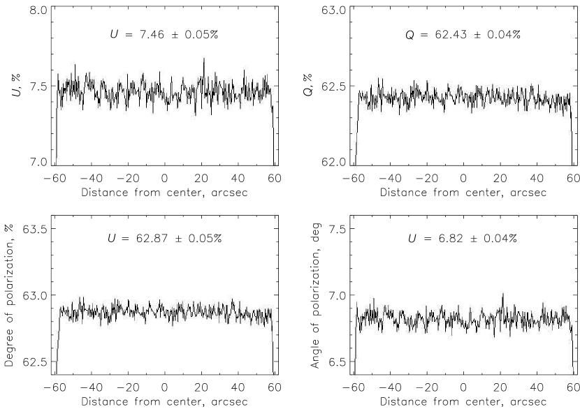
Figure 2: The variations of the Stokes $Q$ and $U$ parameters, the degree of polarization and the angle of the polarization plane based on the observations of the twilight sky.

In the observations with a single Wollaston prism, we register two spectra with the intensity of $I_{o}(\lambda)$ and $I_{e}(\lambda)$ (ordinary and extraordinary, respectively). In general, the orientation of the principal axes of the prism $\varphi$ and the directions of the fast axis vector $\theta$ of the phase plates are arbitrary. Then, as follows from Section 3, the values of the measured, normalized to the integral intensity $I$ Stokes parameters $U$ and $Q$ would be found from the relations:

$$\begin{array}[]{rcl}Q^{\prime}&=&\left[R(\lambda)_{\theta=0\hbox{${}^{\circ}$}}-R(\lambda)_{\theta=45\hbox{${}^{\circ}$}}\right]/2,\\ \\ U^{\prime}&=&\left[R(\lambda)_{\theta=22.5\hbox{${}^{\circ}$}}-R(\lambda)_{\theta=67.5\hbox{${}^{\circ}$}}\right]/2,\\ \end{array}$$ (13)

where $R(\lambda)=\biggl{(}\displaystyle{\frac{I_{o}(\lambda)-I_{e}(\lambda)}{I_{o}(\lambda)+I_{e}(\lambda)}}\biggl{)}$, $\theta$ is the angle of rotation of the $\lambda/2$ phase plate, and the intrinsic values of the second and third Stokes parameters are found from the rotation transformation:

$$\begin{array}[]{rcl}Q/I&=&Q^{\prime}\cos{2\varphi}-U^{\prime}\sin{2\varphi},\\ \\ U/I&=&Q^{\prime}\sin{2\varphi}+U^{\prime}\cos{2\varphi}.\\ \end{array}$$ (14)

The degree of linear polarization $P$ is determined from relation (5), and the observed position angle of the polarization plane ${\rm PA}$ is calculated as follows:

$${\rm PA}={\rm PA}_{\rm slit}-\displaystyle{\frac{1}{2}}\arctan{\displaystyle{\frac{U}{Q}}}+{\rm PA}_{0}.$$ (15)

Here ${\rm PA}_{\rm slit}$ is the position angle of the major axis of the Wollaston prism, which coincides with the direction of the slit, and ${\rm PA}_{0}$ is the zero point of the dependence of the slit position angle on the angle of the BTA primary focus turntable and the parallactic angle of the object. Note that the minus sign in the formula is due to the fact that the image at the entrance of the spectrograph is a reflection of the image on the celestial sphere.

For the measurements of circular polarization, the $\lambda/4$ plate is inserted in the beam, which is oriented in such a way that the direction of the fast axis makes an angle of $45\hbox{${}^{\circ}$}$ with the direction of the main axis of the Wollaston prism. The plate turns by two fixed angles, $0\hbox{${}^{\circ}$}$ and $90\hbox{${}^{\circ}$}$. In this case the value of the circular polarization (the Stokes $V$ parameter) is found from the relation:

$$V/I=\left[R(\lambda)_{\theta=0\hbox{${}^{\circ}$}}-R(\lambda)_{\theta=90\hbox{${}^{\circ}$}}\right]/2.$$ (16)

It is commonly known that this measurement technique allows to eliminate the phase shift errors of the phase plates, but requires a stable atmosphere. In reality though several (more than three) cycles of measurements are carried out during the observations, when we successively record the spectra for pairs of angles ($0\hbox{${}^{\circ}$}$, $45\hbox{${}^{\circ}$}$) and ($22\fdg 5$, $67\fdg 5$) for the $\lambda/2$ plate and ($0\hbox{${}^{\circ}$}$, $90\hbox{${}^{\circ}$}$) for the $\lambda/4$ plate. The duration of the exposure should be at least 3–4 times longer than the CCD frame readout time.

4.2 Double Wollaston Prism

A double Wollaston prism, the concept of which was first proposed and realized by Geyer et al. (Geyer et al., 1996) and developed by Oliva (Oliva, 1997) features two Wollaston prisms inserted at the exit pupil of the spectrograph. One of the prisms, with the directions of polarization axes of $0\hbox{${}^{\circ}$}$ and $90\hbox{${}^{\circ}$}$, is illuminated by one half of the exit pupil, and the other prism, with the directions of axes of $45\hbox{${}^{\circ}$}$ and $135\hbox{${}^{\circ}$}$ is illuminated by the other half of the pupil. Two achromatic wedges were used to separate the images from each prism. Thus, using this registration method, we obtain four spectra with the intensities of $I(\lambda)_{0}$, $I(\lambda)_{90}$, $I(\lambda)_{45}$, and $I(\lambda)_{135}$.

Then, the values of the second and third normalized Stokes $Q$ and $U$ parameters are determined from the relations:

$$\begin{array}[]{rcl}Q^{\prime}&=&\displaystyle{\frac{I(\lambda)_{0}-I(\lambda)_{90}}{I(\lambda)_{0}+I(\lambda)_{90}}},\vspace{-5mm}\\ \\ \\ U^{\prime}&=&\displaystyle{\frac{I(\lambda)_{45}-I(\lambda)_{135}}{I(\lambda)_{45}+I(\lambda)_{135}}}.\\ \end{array}$$ (17)

For the measurement of circular polarization the $\lambda/4$ phase plate is inserted in the beam and then

$$\begin{array}[]{rl}V/I=0.5\biggl{(}\displaystyle{\frac{I(\lambda)_{0}-I(\lambda)_{90}}{I(\lambda)_{0}+I(\lambda)_{90}}}\biggr{)}&\vspace{-5mm}\\ \\ \\ -0.5\biggl{(}\displaystyle{\frac{I(\lambda)_{45}-I(\lambda)_{135}}{I(\lambda)_{45}+I(\lambda)_{135}}}\biggr{)}&\!\!.\\ \end{array}$$ (18)

The values of the Stokes $U$ and $Q$ parameters, and the position angle of the polarization plane ${\rm PA}$ are calculated here using the (14) and (15) relations, and the degree of polarization $P$ is found from formula (5).

This measurement method, as opposed to the previous one, provides for a simultaneous measurement of the Stokes $Q$ and $U$ parameters, which is important in the conditions of unstable atmosphere. However, its disadvantage is the need to calibrate the sensitivity of four independent polarization channels by the zero polarization standard. Although the calibration dependences $I(\lambda)_{0}/I(\lambda)_{90}$ and $I(\lambda)_{45}/I(\lambda)_{135}$ are constant for the instrument, nevertheless, they have to be refined on each night of observations.

4.3 Dichroic Polarization Analyzer

The dichroic polarization analyzer (also called the polarization filter or the polaroid), mounted in the spectrograph is intended for the measurements of linear polarization in starlike and extended objects in the field of view with the diameter of 6^′. It is also planned to be used for two-dimensional spectropolarimetry after the commissioning of the integral field spectroscopy mode at the SCORPIO-2 spectrograph.

The analyzer can be set in three fixed positions by the angle, $0\hbox{${}^{\circ}$}$ and $\pm 60\hbox{${}^{\circ}$}$. Then, with intensities measured in three angles of the polaroid, $I(x,y)_{0\hbox{${}^{\circ}$}}$, $I(x,y)_{-60\hbox{${}^{\circ}$}}$ and $I(x,y)_{+60\hbox{${}^{\circ}$}}$ we can calculate, up to the rotation transform, the measured Stokes $Q^{\prime}$ and $U^{\prime}$ parameters in each point of the image with the coordinates $(x,y)$:

$$\begin{array}[]{rcl}Q^{\prime}(x,y)&=&\displaystyle{\frac{2I(x,y)_{0}-I(x,y)_{-60}-I(x,y)_{+60}}{I(x,y)_{0}+I(x,y)_{-60}+I(x,y)_{+60}}},\vspace{-5mm}\\ \\ \\ U^{\prime}(x,y)&=&\displaystyle{\frac{1}{\sqrt{3}}\frac{I(x,y)_{+60}-I(x,y)_{-60}}{I(x,y)_{0}+I(x,y)_{-60}+I(x,y)_{+60}}}.\\ \end{array}$$ (19)

The values of the Stokes $Q$ and $U$ parameters, the degree of linear polarization $P$ and the position angle of the polarization plane ${\rm PA}$ are calculated here from relations (14), (5) and (15), respectively. This measurement technique was proposed by Fesenkov, but out of three observed intensity values he only computed the degree of polarization and the rotation angle of the polarization plane  (Dombrovsky, 1957). Just like in the case of the single Wollaston, this measurement technique depends on the atmospheric conditions.

4.4 Generation of the Initial Data Cube

A common problem encountered in the reduction of polarimetric observations is that when we compare the differential values in each image point, any, even very small differences between the images obtained at different angles of the phase plates or the polaroid, which are introduced at various stages of the reduction, impair the accuracy of polarization measurements. The same applies to the removal of the traces of cosmic ray particles by different smoothing techniques, since these algorithms typically shift the statistic estimates, and therefore contribute some depolarization effects to the final result.

A large amount of different images is generated, obtained at various angles of phase plates, possessing different features (obj, flat, bias, neon, dark, etalon) and types of observed objects (the studied object, the zero polarization standard, the non-zero polarization standard). This calls for a uniformity of the input data fed to the reduction software with the minimal intervention of the astronomer. To this end, the reduction software first analyzes the FITS-headings of the input array of images and generates the following data:

• 1) $\tt obj(x,y,pol,exp)$ is the 4-dimensional cube of initial data, where $\tt x,y$ are coordinates of the point on the image, $\tt pol$ is the identifier of the phase plate and its angle:

  $$\begin{array}[]{ll}{\tt pol}=0\rightarrow\lambda/2\,(0\hbox{${}^{\circ}$}),&{\tt pol}=1\rightarrow\lambda/2\,(45\hbox{${}^{\circ}$}),\\ {\tt pol}=2\rightarrow\lambda/2\,(22\fdg 5),&{\tt pol}=3\rightarrow\lambda/2\,(67\fdg 5),\\ {\tt pol}=4\rightarrow\lambda/4\,(0\hbox{${}^{\circ}$}),&{\tt pol}=5\rightarrow\lambda/4\,(90\hbox{${}^{\circ}$}),\\ \lx@intercol\hfil{\tt pol}=6\rightarrow{\rm polaroid}\,(0\hbox{${}^{\circ}$}),\phantom{+6}\hfil\lx@intercol\\ \lx@intercol\hfil{\tt pol}=7\rightarrow{\rm polaroid}\,(+60\hbox{${}^{\circ}$}),\hfil\lx@intercol\\ \lx@intercol\hfil{\tt pol}=8\rightarrow{\rm polaroid}\,(-60\hbox{${}^{\circ}$});\hfil\lx@intercol\\ \end{array}$$

  and ${\rm exp}$ is an identifier that determines the type of the object and the number of the exposure;

• 2) $\tt bias(x,y)$ is a robust estimate of the electrical zero of the registration system;

• 3) $\tt neon(x,y,pol)$ is the image of the line spectrum for the wavelength scale calibration;

• 4) $\tt flat(x,y,pol)$ is the image of the spectra of a continuous-spectrum lamp used for the transmission calibration.

The subsequent data processing steps involve the construction of a model of scale distortions, reduction of data for these distortions and the sensitivity heterogeneity, the sky background subtraction, the wavelength scale calibration, extraction of the spectra from the images (or the integral fluxes from the objects, given the field photometry), and finally, the calculation of the Stokes parameters. The removal of the traces of cosmic ray particles is done at the final stage of reduction via the robust parameter estimates.

4.5 Correction of Scale Distortions

The images obtained in the 2D-spectropolarimetry mode are strongly distorted for various reasons:

• 1) the spectral line curvature along the slit height, caused by the variation of the meridional increase of dispersion elements used in the spectrograph, namely, the Volume Phase Holographic Gratings (VPHG) combined with prisms;

• 2) the chromatism of the Wollaston prism, leading to the wavelength-dependent value of the divergence of ordinary and extraordinary rays, which increases the curvature of spectral trajectories, as compared with the conventional spectroscopy;

• 3) the distortion of the spectrograph camera optics and the higher order spherical chromatic aberrations also leading to the geometric distortions.

The value of geometric distortions in our case can reach up to 10–15% in the observations covering a wide spectral range. Given that in the case of accurate measurements the errors of the Stokes parameters should not exceed 0.1%, the final coordinate-wise nonlinearity of data in the spectra cannot exceed 0.1 px, what corresponds to about 0.005% for the CCD we use ($2068\times 4632$ px). In order to obtain such a high accuracy, the scale distortions have to be carefully calibrated, and exact algorithms of coordinate conversion have to be applied.

As a model of geometric transformations, we use the geometric polynomial $N$-order transformation, where the resulting set of intensity values is determined by the following relations:

$$I[x,y]=I^{\prime}[x^{\prime},y^{\prime}]=I^{\prime}[a(x,y),b(x,y)]~{},$$ (20)

where $I[x,y]$ is the intensity in the point with the coordinates $(x,y)$ in the undistorted image, which corresponds to the intensity $I^{\prime}[x^{\prime},y^{\prime}]$, measured in the point of the distorted image with the coordinates $(x^{\prime},y^{\prime})$.

The functions $a(x,y)$ and $b(x,y)$ are the polynomials of the $N$th degree, whose coefficients $K_{x_{i,j}}$ and $K_{y_{i,j}}$ determine the spatial transformation:

$$x^{\prime}=a(x,y)=\sum_{i=0}^{N}\sum_{j=0}^{N}K_{x_{i,j}}x^{j}y^{i}$$ (21)

$$y^{\prime}=b(x,y)=\sum_{i=0}^{N}\sum_{j=0}^{N}K_{y_{i,j}}x^{j}y^{i}.$$ (22)

The accuracy of the model of geometric distortions depends on the accuracy of determining the $K_{x_{i,j}}$ and $K_{y_{i,j}}$ coefficients. From this point on, we consider that the degree of the polynomial, responsible for our distortions, is not higher than three, and the resulting coordinates of nodes are accurate, so that the spline interpolation could be used in the geometric transformation. It should also be noted that the accuracy of the geometrical model determines the quality of the night sky spectrum subtraction, which is important for the polarization observations of faint objects.

The model of distortions is constructed as follows.

Figure 3: The trajectories of the etalon spectra for the single Wollaston prism.

First, based on the analysis of the etalon spectra (which is an image of the individual spectra of the continuous-spectrum lamp, given that a dot mask is inserted in front of the slit) the curvature of the spectra along dispersion is determined, which we shall further call the trajectories of the spectra.

1) First, based on the analysis of the etalon spectra (which is an image of individual spectra of a continuous-spectrum lamp, given that a dot mask is inserted in front of the slit) the curvature of the spectra along dispersion is determined, which we shall further call the trajectories of the spectra. For the single and double Wollaston prisms, a 5- and a 3-dot mask is inserted in front of the slit, respectively. Figure 3 shows an example of construction of the trajectories for the image of the standard obtained with a single Wollaston prism. The positions of nodes are determined from the analysis of spectral sections across dispersion. The positions of the obtained points are approximated by the polynomial of the third degree, which gives the true shape of the trajectories.

2) Then, the obtained trajectories are superimposed over the two-dimensional image of the comparison spectrum to determine the positions of spectral lines at the nodes of their intersections with the trajectories. Out of the entire array of the obtained intersections we determine the points, coinciding by wavelength for each trajectory. Based on them, a model of the curvature along the slit height is constructed for each line using the third-degree polynomial. An example of identification of spectral lines and the approximation of their curvature by the third-degree polynomials is shown in Fig. 6. At that, an individual polynomial is constructed for each identified line.

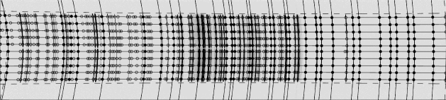
Figure 4: The approximation of the curvature of the comparison spectrum lines by the third-degree polynomials for the single Wollaston prism.

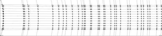
Figure 5: The nodes of the grid of the geometric distortion model. The crosses and points mark the undistorted and distorted images, respectively.

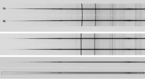
Figure 6: Image processing with a single Wollaston prism: the top plot represents the original spectrum, the middle plot—the spectrum, corrected for the geometric distortions, and the bottom plot presents the spectrum after the background sky subtraction.

3) At last, at the final stage the obtained coefficients of the polynomials, defining the curvature of the lines and trajectories are approximated by wavelength by the second-degree polynomial, and based on the results of approximation of these coefficients the smoothed curved lines and trajectories of the spectra are constructed. Next, the points of intersection $(x^{\prime},y^{\prime})$ of line trajectories are computed. Here, the $x$-coordinates of lines and the $y$-coordinates of the trajectory in the center of the image are regarded as the true (undistorted) coordinates $(x,y)$. The exact coordinates of the nodes obtained by these means are used to determine the two-dimensional polynomial coefficients, found from the expressions (21) and (22). At the edges of the image of the spectrum the nodes are extrapolated according to the approximation of the curvature of lines and trajectories. The result of constructing the nodes of the geometrical model grid in the image is demonstrated in Fig. 6.

Next, all the original images (obj, flat, neon) are corrected for the geometric distortions using the IDL environment WARP_TRI procedure, the corrections for the sensitivity heterogeneity are done (the flat-field procedure) and the sky background is subtracted. Our numerous tests have shown that the actual accuracy of the correction for geometric distortions is at least 0.2 px, what corresponds to $3\mu$m in the plane of the CCD. The examples of images at various stages of reduction of data, obtained with the single Wollaston prism are shown in Fig. 6.

The wavelength scale calibration is performed is a standard way: automatic line identification, two-dimensional approximation of the dispersion curve by the third-order polynomial, quadratic smoothing of the polynomial coefficients along the slit height, and image linearization.

4.6 Extraction of Spectra and Calculation of the Stokes Parameters

Figure 7: The spectrum of the nucleus of the Markarian 6 galaxy, extracted from the image in Fig. 6.

The accuracy of calculation of the Stokes parameters, besides the exactness of geometric transformations, depends on how the dimensionless quantities $R(\lambda)$, participating in the relations (13), (16), (17) and (18) are determined. In case of the observations of extended objects, the above equations involve the intensity values of the ordinary and extraordinary rays $I_{\rm o}(x,y)$ and $I_{\rm e}(x,y)$, which are used to calculate the Stokes parameters at each point in the image. The mean Stokes parameter value for each position along the slit (up to the image size) is calculated by the robust methods using the stellar image profile at the entrance of the spectropolarimeter as a scaling function. However, in the case of starlike objects we have to use the methods similar to the aperture photometry techniques (Stetson et al., 1998), which allow to extract the spectrum of the object from the image in an optimal way (in terms of the maximum signal-to-noise ratio), and also do not introduce any dummy instrumental polarization. Moreover, the impulse interferences in the image, mainly brought in by the cosmic ray particles, are efficiently suppressed. An example of the spectrum extraction is shown in Fig. 7.

For the optimal extraction of the spectra, the approximation of the stellar profile along the slit (by the $y$-coordinate) according to the Moffat model (Moffat, 1969) is generally applied:

$${\rm PSF}(y)=a_{0}+\displaystyle{\frac{a_{1}}{(u+1)^{a_{6}}}},$$ (23)

where $u=\displaystyle{\biggl{(}\frac{y-a_{4}}{a_{2}}\biggr{)}^{2}+\biggl{(}\frac{y-a_{4}}{a_{2}}\biggr{)}^{2}}$. In more complex cases, the profile is approximated by a combination of Gaussian functions.

4.7 Atmospheric Condition Monitoring

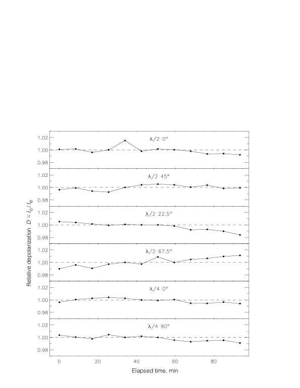
Figure 8: The variation of the depolarization coefficients $D=I_{o}/I_{e}$ normalized for the median value for the successive 60-s exposures with the step of 100 s in the observations with a single Wollaston prism.

One of the most serious factors limiting the accuracy of the ground-based polarization observations is the effect of the Earth’s atmosphere. A simple transparency variation in the case of the double-beam scheme of polarization measurements has little effect on the accuracy of measurement of the normalized Stokes parameters. However, the variation of the parameters of the radiative transfer in the atmosphere leads to an adjustment of the depolarization coefficient $D=I_{\rm o}/I_{\rm e}$ at different exposures, what is illustrated in Fig. 8. The main reason of depolarization is the selective light scattering from single microparticles that are smaller than the wavelength of the observed radiation (the Rayleigh scattering with magnitude proportional to $\lambda^{-4}$), and non-selective aerosol light scattering (Chen et al., 2003). In the case of observations from the BTA location, where the atmosphere is dominated by the aerosol scattering (Kartashova & Chunakova, 1978), we can expect that the effects of depolarization will depend little on wavelength. Moreover, the characteristic times of the fast depolarization variations in the atmosphere are comparable with the the exposure times short enough to “freeze” the atmospheric turbulence, and, depending on the atmospheric conditions during the observations, amount to about 10–30 ms. To suppress the effects of depolarization (which are called the scintillation effects) the schemes with a fast modulation or polarization channel switching are generally applied. In spectropolarimetry this is only possible with the use of the KDP crystals and only for bright objects, since such schemes have an extremely low transmission.

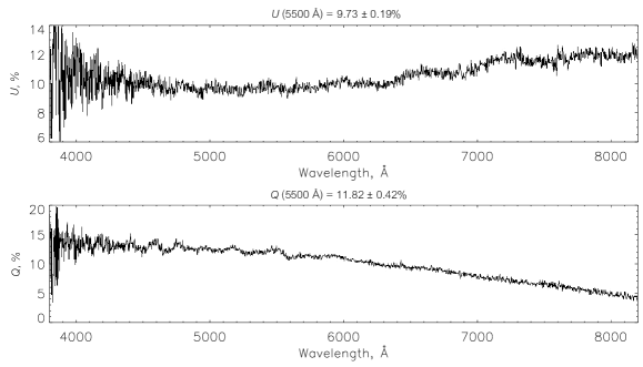
Figure 9: The influence of depolarization effects on the wavelength dependence of the Stokes parameters for the blazar S5 0716+71.

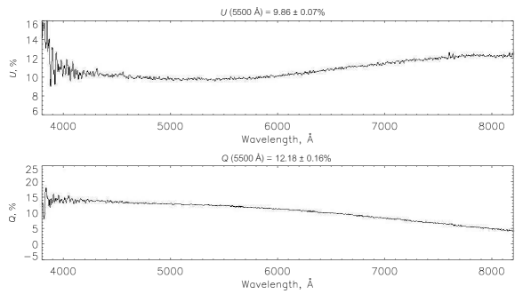
Figure 10: The wavelength dependence of the Stokes parameters for the blazar S5 0716+71 after the correction for the depolarization effects in the Earth’s atmosphere.

Table 1: A comparison of the measured parameters of linear polarization for WOLL-1

Star	$P_{\rm obs}$,%	$P_{\rm tab}$,%	$\rm PA_{obs}$, deg	$\rm PA_{tab}$, deg
BD +58∘2272	$5.52\pm 0.07$	$5.49\pm 0.02$	$58.4\pm 0.7$	$59.3\pm 0.1$
HD 14433	$3.65\pm 0.07$	$3.77\pm 0.01$	$113.7\pm 0.5$	$112.9\pm 0.3$
BD +59∘385	6.76 $\pm$ 0.06	6.70 $\pm$ 0.02	96.5 $\pm$ 0.8	98.1 $\pm$ 0.1
Hiltner 960	$5.70\pm 0.13$	$5.66\pm 0.02$	$56.3\pm 0.6$	$54.5\pm 0.2$
Hiltner 960	$5.86\pm 0.14$	$5.66\pm 0.02$	$53.5\pm 0.3$	$54.5\pm 0.2$
HD 7927*	$3.02\pm 0.07$	$3.30\pm 0.03$	$90.8\pm 0.8$	$91.1\pm 0.2$
HD 204827*	$5.15\pm 0.14$	$5.32\pm 0.01$	$57.7\pm 0.8$	$58.7\pm 0.8$
BD +64∘106*	$5.18\pm 0.10$	$5.69\pm 0.04$	$94.8\pm 0.9$	$96.6\pm 0.2$

Table 2: A comparison of the measured parameters of linear polarization for WOLL-2

Star	$P_{\rm obs}$,%	$P_{\rm tab}$,%	$\rm PA_{obs}$, deg	$\rm PA_{tab}$, deg
HD 15597	$4.50\pm 0.27$	$4.38\pm 0.03$	$102.9\pm 1.7$	$103.2\pm 0.3$
HD 15597*	$4.13\pm 0.33$	$4.38\pm 0.03$	$100.1\pm 2.6$	$103.2\pm 0.3$
HD 154445*	$3.14\pm 0.24$	$3.67\pm 0.05$	$84.1\pm 5.1$	$88.6\pm 0.7$
HD 161056	$4.02\pm 0.19$	$4.00\pm 0.01$	$66.2\pm 1.4$	$66.3\pm 0.3$
VI Cyg-12	$8.97\pm 0.07$	$8.95\pm 0.09$	$115.2\pm 1.2$	$115.0\pm 0.3$
Hiltner 960	$5.76\pm 0.14$	$5.66\pm 0.02$	$53.5\pm 1.5$	$54.8\pm 0.2$
HD 204827*	$5.11\pm 0.19$	$5.34\pm 0.02$	$58.1\pm 1.3$	$58.7\pm 0.8$

Figure 10 shows the effect of depolarization by the Earth’s atmosphere on the variation of the wavelength dependence of the Stokes $U$ and $Q$ parameters in the S5 0716+71 blazar with the synchrotron emission mechanism. It should be noted that the spectra presented in Fig. 10 are wavelength-modulated, which must not be since the synchrotron radiation produces smooth wavelength dependences of the Stokes parameters. If we interpret the variation of depolarization during the observations (see Fig. 8) as a variation of the spectrograph transmission for the ordinary and extraordinary rays, then in the expression (13) instead of $\biggl{(}\displaystyle{\frac{I_{\rm o}(\lambda)-I_{\rm e}(\lambda)}{I_{\rm o}(\lambda)+I_{\rm e}(\lambda)}}\biggr{)}_{k}$ we should use $\biggl{(}\displaystyle{\frac{D_{k}I_{\rm o}(\lambda)-I_{\rm e}(\lambda)}{D_{k}I_{\rm o}(\lambda)+I_{\rm e}(\lambda)}}\biggr{)}_{k}$, where $k$ is the number of the corresponding exposure, and the depolarization coefficients $D_{k}$ are taken from the observed deviations relative to the mean (Fig. 8). The result of computation of the Stokes parameters with the atmospheric depolarization corrected this way is shown in Fig. 10.

As shown in Fig. 10, the result exceeds the most audacious expectations—the modulation of the $U$ and $Q$ spectra is completely eliminated, while the statistical measurement error has decreased 2.5-fold and corresponds to that, expected for the Poisson statistics! This is a direct indication that the discovered technique of correction for the depolarization effects in the Earth’s atmosphere caused by the scintillations is correct. It should certainly be borne in mind that firstly, it is applicable for the objects in which the times of internal (intrinsic to the object) variability are longer than the total exposure time, and secondly, this technique does not account for the average degree of depolarization in the atmosphere. However, it (the average degree of depolarization) can be determined from the observations of the polarization standard stars before and after the object at the same zenith distances.

5 RESULTS OF TEST OBSERVATIONS

For the pilot observations of linear polarization we used the polarization standard stars from the lists of Hsu and Breger (Hsu & Breger, 1982), and Turnshek et al. (Turnshek, 1990). The observations were conducted in two polarization modes, WOLL-1 and WOLL-2. Whenever possible during each night of observations, the zero-polarization standards were recorded to control the instrumental polarization, and the non-zero polarization standards were registered to refine the zero-point of the position angle of the polarization plane. The spectra were obtained in the range of 3700–8300 Å with the spectral resolution of about 12 Å with the Volume Phase Holographic Grating VPHG940@600. After the series of reductions, the sequence of which is described in the previous section, the normalized Stokes vectors $Q(\lambda)$ and $U(\lambda)$ were obtained for each star. The robust estimates of the Stokes parameters in the photometric V-band were made taking account of the standard V$(\lambda)$ curve. Next, using the (5) and (15) relations, we calculated the average values of the observed polarization $P_{\rm obs}$ and the angle of the polarization plane $\rm PA_{obs}$ in the photometric V-band, which are listed in Table 1. The same table gives the true values of $P_{\rm tab}$ and $\rm PA_{tab}$, adopted from (Hsu & Breger, 1982) and (Turnshek, 1990).

The estimates made during the night with unstable atmospheric conditions (cirri) are marked with an asterisk in the table. The estimates of polarization of standard stars demonstrated the absence of significant linear instrumental polarization within the errors (of about 0.1%). As we can see from the table, the quality of data we have acquired varies greatly. On the nights with good transparency the true accuracy of linear polarization measurements reaches 0.05% in the observations using the WOLL-1 polarization filter.

In cases where the transparency was not exceptional, and depolarization reached 2–3%, the observations were conducted only with the double Wollaston prism (WOLL-2), which yielded the measurement accuracy of about 0.2%, what is well illustrated by the data from Table 2, listing the measurements of the polarization standards with WOLL-2.

6 CONCLUSION

The test observations and their analysis imply that the proposed technique allows obtaining real values of polarization and making sufficiently reliable estimates of their errors. Note in particular that the proposed technique, given all the difficulties of performing the polarimetric measurements, allows for the measurements of linear and circular polarization in rather difficult weather conditions. The observations of extended objects in our case are not aggravated by the presence of the variable instrumental polarization along the slit. This makes our technique especially promising for the studies of faint starlike and extended objects.