Algebraic geometry of Poisson regression

Abstract.

Designing experiments for generalized linear models is difficult because optimal designs depend on unknown parameters. Here we investigate local optimality. We propose to study for a given design its region of optimality in parameter space. Often these regions are semi-algebraic and feature interesting symmetries. We demonstrate this with the Rasch Poisson counts model. For any given interaction order between the explanatory variables we give a characterization of the regions of optimality of a special saturated design. This extends known results from the case of no interaction. We also give an algebraic and geometric perspective on optimality of experimental designs for the Rasch Poisson counts model using polyhedral and spectrahedral geometry.

1. Introduction

Generalized linear models are a mainstay of statistics, but optimal experimental designs for them are hard to find, as they depend on the unknown parameters of the model. A common approach to this problem is to study local optimality, that is, determine an optimal design per fixed set of parameters. In practice, this means that appropriate parameters have to be guessed a priori, or fixed by other means. Here we take a global view on the situation. Our goal is to partition parameter space into regions of optimality, such that in each region the optimal design is (at least structurally) constant. Our key observation is that, by means of general equivalence theorems, the regions of optimality are often semi-algebraic, that is, defined by polynomial inequalities. This opens up the powerful toolbox of real algebraic geometry to the analysis of optimality of experimental designs.

We discuss the phenomenon on the Rasch Poisson counts model, a certain generalized linear model that appears in Poisson regression, for example in tests of mental speed in psychometry [6]. The parameterization of the intensities of the Poisson distribution is akin to the toric models in algebraic statistics. The view from experimental design, however, is new, and the resulting mathematical questions have not been considered in algebraic statistics. Our main result is a characterization of optimality of a particular saturated design in Theorem 3.3. Beyond that, we also demonstrate how to approach the problem from a geometric point of view. In particular, in Section 4 we describe the problem of determining regions of optimality in the language of mathematical optimization. We are convinced that interesting mathematical structures can be found when studying the polynomial inequalities that arise from the different equivalence theorems in the theory of optimal experimental design.

Acknowledgement

TK is supported by the Research Focus Dynamical Systems (CDS) of the state Saxony-Anhalt. We thank Bernd Sturmfels for sharing his geometric view on the problem, leading to some of the considerations in Section 4.

Notation

We switch freely between a binary vector ${\mathbf{x}}=(x_{i})\in\{0,1\}^{k}$ and a subset $A\subset\{1,\dots,k\}$. If confusion can arise, the subset corresponding to ${\mathbf{x}}\in\{0,1\}^{k}$ is written $A({\mathbf{x}})=\{i:x_{i}=1\}$, and conversely, the binary vector for a given $A$ is ${\mathbf{x}}(A)$ with components $x_{i}(A)=1$ if $i\in A$ and $x_{i}(A)=0$ otherwise.

2. The Rasch Poisson counts model

When testing mental speed, psychometrists often present series of questions and count the number $Y$ of correctly solved items in a fixed time. One example of such a test is the Münster Mental Speed Test [6]. In such a setting it is natural to model the response $Y$ as Poisson distributed with parameter $\lambda>0$, often called the intensity. According to the basic principle of statistical regression, the mean of the response $Y$ (which is just $\lambda$) is a deterministic function of the factors of influence. Rasch’s idea was to make $\lambda=\theta\sigma$ multiplicative in the ability $\theta$ of a test person and the easiness $\sigma$ of the tasks. Due to the multiplicative structure, an absolute estimation of either ability or easiness is only possible if the other quantity is fixed. For the mathematics, the distinction between $\theta$ and $\sigma$ is not relevant, because we make another multiplicative ansatz for $\sigma$ below, and $\theta$ may well be subsumed there.

Rule based item generation is a computer driven mechanism to generate questions to present to the subjects. One question’s easiness $\sigma({\mathbf{x}})$ depends on a rule setting ${\mathbf{x}}$. We think of the rules as discrete switches that can be on or off and that influence the difficulty of the question. In practice, we often assume that each additional rule makes the task harder and thus decreases the intensity. Throughout the paper, the number of rules is fixed as $k\in\mathbb{N}$. The possible experimental settings are thus the binary vectors ${\mathbf{x}}=(x_{1},\ldots,x_{k})\in\{0,1\}^{k}$ (but see our Notation section).

The natural choice for the influence of rule settings on the intensity $\lambda$ is exponential:

(2.1) $$\lambda({\mathbf{x}})=\theta\sigma({\mathbf{x}})=\exp(f({\mathbf{x}})^{T}\beta)$$

for a vector of regression functions $f:\{0,1\}^{k}\to\mathbb{R}^{p}$, and a vector of parameters $\beta\in\mathbb{R}^{p}$. A concrete model is specified by means of the integers $k,p$, and the regression functions $f$.

Definition 2.1.

The interaction model of order $d$ is specified by the regression function

(2.2) $$f_{d}({\mathbf{x}})=(\text{all squarefree monomials of degree at most $d$ in $x_{1},\dots,x_{k}$})$$

Remark 2.2.

If our rule settings ${\mathbf{x}}$ were not binary, then in Definition 2.1 there would be a difference between using all monomials and all squarefree monomials. For binary ${\mathbf{x}}$ there is none since $x_{i}^{2}=x_{i}$ for all $i$.

Example 2.3.

The most interesting model from a practical perspective is the independence model which arises for $d=1$. In this case $f({\mathbf{x}})=(1,x_{1},\dots,x_{k})$ and $p=1+k$. The pairwise interaction model arises for $d=2$, where $f({\mathbf{x}})=(1,x_{1},\dots,x_{k},x_{1}x_{2},\dots,x_{k-1}x_{k})$ and $p=1+k+\binom{k}{2}$. Somewhat confusingly this second situation is sometimes called first order interaction.

Definitions (2.1) and (2.2) lead to a product structure for the intensity $\lambda({\mathbf{x}})$ as follows. Let $d\geq 1$. There is a parameter $\beta_{A}$ for each $A\subset\{1,\dots,k\}$ with $|A|\leq d$. Then

(2.3) $$\lambda({\mathbf{x}},\beta)=\prod_{\begin{subarray}{c}A\subset A({\mathbf{x}})\\ |A|\leq d\end{subarray}}e^{\beta_{A}}.$$

Hence, the more rules are applied, the more terms $e^{\beta_{A}}$ enter the product (2.3). In the $d=1$ case, there is one term $e^{\beta_{\{i\}}}$ for each $i\in\{1,\dots,k\}$ and one global term $\beta_{\emptyset}$. The intensity is then proportional to the product over those terms for which the corresponding rule is active and there is no interaction among the rules. For higher interaction order $d$, if, for example, rules $1,2$ are active, the corresponding factor is $e^{\beta_{\{1\}}}e^{\beta_{\{2\}}}e^{\beta_{\{1,2\}}}$, etc. If all singleton parameters $\beta_{\{i\}}$ have the same sign, then having a parameter $\beta_{A},|A|\geq 2$ with the same sign is sometimes called synergetic interaction, while $\beta_{A}$ with a different sign is called antagonistic interaction.

The case $d=1$ is particularly well-behaved (and very relevant for the practitioners). Graßhoff, Holling, and Schwabe have investigated this case in depth in [8, 9, 10]. In Section 3 we generalize some of their results to the general interaction case.

Remark 2.4.

In (2.2) we chose all squarefree monomials of bounded degree. Therefore, if there is a parameter $\beta_{A}$ for some set $A$ of rules, then there also are parameters $\beta_{B}$ for all subsets $B$ of $A$. In the language of combinatorics, the indices of the parameters form a simplicial complex, and one could conversely define a model for each simplicial complex, by letting the regression function consist of squarefree monomials corresponding to the faces of the complex. This puts our parametrizations of possible intensities $\lambda$ in the context of hierarchical log-linear models [7, Section 1.2], certain hierarchically structured exponential families that also arise in the theory of information processing systems [12].

Remark 2.5.

In (2.1), not all vectors $\lambda\in\mathbb{R}^{2^{k}}$ have corresponding parameters $\beta$. Obviously, $\lambda$ needs to have positive entries, but there are further restrictions. For the simplest example, in the case $k=2,d=1$, there are four possible rule settings $\{(00),(01),(10),(11)\}$. Independent of the parameters $\beta$, it holds that

$$\lambda(00)\lambda(11)-\lambda(10)\lambda(01)=0,$$

since both terms equal $e^{2\beta_{\emptyset}}e^{\beta_{1}}e^{\beta_{2}}$. As a function $\mathbb{R}^{4}\to\mathbb{R}$, this $2\times 2$ determinant vanishes identically on the image of the parametrization and it can be seen that this vanishing characterizes points in the image. For any $k$ and $d$, there is a finite set of binomials (that is, polynomials with only two monomials) in $\lambda$ that characterizes the image of the parameterizations. In commutative algebra these are known as the generators of certain toric ideals [19, Chapter 4], while in algebraic statistics they are called Markov bases [5]. In principle, after fixing $k$ and $d$, all binomials can be computed with the help of computer algebra (the fastest software is 4ti2 [1]), but this is hard already for $d=2$ and $k>7$. Many special cases have been dealt with in algebraic statistics, though. See [2] and references therein.

2.1. Optimal experimental design

The estimation problem is to determine the values of the parameters $\beta$ given observations $(Y^{(i)},{\mathbf{x}}^{(i)})$, $i=1,\dots,N$ which are pairs of experimental settings ${\mathbf{x}}^{(i)}$ and responses $Y^{(i)}$. As $Y$ is a random variable, the estimator is a random variable too. In practice, when designing an experiment to determine $\beta$, we can choose which settings ${\mathbf{x}}^{(i)}$ to present. This choice should be made so that the result of the experiment is most informative about $\beta$. Doing so, we may also choose to test a particular setting ${\mathbf{x}}$ multiple times. This quickly leads to an idea of Kiefer: An approximate design is a vector $(w_{\mathbf{x}})_{{\mathbf{x}}\in\{0,1\}^{k}}\in[0,1]^{2^{k}}$ of non-negative weights with $\sum_{\mathbf{x}}w_{\mathbf{x}}=1$. In the following we only work with approximate designs as our choices of experimental settings.

How is the quality of a design to be measured? Quite generally, one uses the Fisher information matrix, defined as

(2.4) $$M(w,\beta)=\sum_{{\mathbf{x}}\in\{0,1\}^{k}}w_{\mathbf{x}}\lambda({\mathbf{x}},\beta)f({\mathbf{x}})f({\mathbf{x}})^{T}.$$

This choice can be motivated by large sample asymptotics: asymptotically the maximum-likelihood-estimator of the parameters is normal and its standardized covariance matrix is the inverse of the Fisher information. An optimality criterion is any function that produces a real number from the Fisher information. Here we choose the popular $D$-optimality criterion which uses the determinant. The design problem for the Poisson counts model is to determine descriptions of the regions in $\beta$-space where certain designs are optimal. Given a particular design, however, there may be no parameters $\beta$ for which this design is optimal.

Remark 2.6.

When the global parameter $\beta_{\emptyset}$ changes, the determinant of $M(w,\beta)$ is globally scaled. For all question regarding optimal design we may therefore assume $\beta_{\emptyset}=0$.

Example 2.7.

If $\beta_{A}=0$ for all $A$, one can check that the situation reduces to that of a linear model. A $D$-optimal experimental design is given by the uniform weight vector $w_{\mathbf{x}}=\frac{1}{2^{k}}$, for all ${\mathbf{x}}\in\{0,1\}^{k}$.

2.2. Symmetry

The regions of optimality show a high degree of symmetry. We use only basic facts about symmetric designs. Corresponding statements can be made in more general settings [18]. Let $G$ be a finite group acting on the set of design points $\{0,1\}^{k}$. Two natural symmetries result from $G=S_{k}$, the symmetric group permuting rules, and $G=\mathbb{Z}_{2}^{k}$ whose elements exchange the roles of $0$ and $1$ for some rules. The action $\circ$ of $G$ on approximate designs is defined by $(g\circ w)_{\mathbf{x}}=w_{g\circ{\mathbf{x}}}$. A crucial assumption for the exploitation of symmetry in design theory is that the action of $G$ induces a linear action on regression functions, that is, for each $g\in G$ there is a matrix $Q_{g}$ such that $f(g\circ{\mathbf{x}})=Q_{g}f({\mathbf{x}})$. It is not difficult to assert this assumption in our case. From this one can define a corresponding action (also denoted $\circ$) on parameter space via the requirement $f(g\circ{\mathbf{x}})^{T}(g\circ\beta)=f({\mathbf{x}})^{T}\beta$ that the response be invariant. It is obvious that $g\circ\beta=Q_{g}^{-T}\beta$ is a possible choice. By linearity, and since the intensity $\lambda({\mathbf{x}},\beta)$ only depends on the response $f({\mathbf{x}})^{T}\beta$, information matrices transform as

$$M(g\circ w,g\circ\beta)=Q_{g}M(w,\beta)Q_{g}^{T}.$$

Since $G$ is finite, $Q_{g}$ is unimodular and the determinant is unchanged. This proves that any optimal design $w$ for parameters $\beta$ yields the optimal design $g\circ w$ for parameters $g\circ\beta$: if a better value was possible in the optimization problem for parameters $g\circ\beta$, then a better value of the determinant could also be achieved in the problem for $\beta$. In total we have the following proposition.

Proposition 2.8.

The regions of optimality are symmetric in the sense that if $w$ is a $D$-optimal approximate design for parameters $\beta$, then $g\circ w$ is a $D$-optimal approximate design for parameters $g\circ\beta$.

Example 2.9.

If $d=1$, and $G=\mathbb{Z}_{2}^{k}$ consists of $0/1$ exchanges, then it is easy to check that the matrices $Q_{g}$ correspond to sign changes on the parameters $\beta$. In particular, the regions of optimality are point symmetric around the origin.

Another way to study the symmetry in this optimization problem is to compute the determinant of the information matrix explicitly. For example, if $d=1$, exchanging $\beta_{i}$ by $-\beta_{i}$ replaces $\lambda_{i}$ by $1/\lambda_{i}$ so that homogeneity of the determinant can be exploited to see the symmetry. For $d=1,k=2$, the determinant is equal to the elementary symmetric polynomial of degree three in the products $w_{{\mathbf{x}}}\lambda({\mathbf{x}})$. For $d=1$ and higher values $k$, the determinant is not an elementary symmetric polynomial (it misses monomials) but it still has a nice combinatorial description. It is an interesting exercise to work out the relation between the determinant and the matrices $Q_{g}$ from above also for $d>1$.

3. Semi-algebraic regions of optimality for saturated designs

The number of parameters of our interaction model of order $d$ equals $p=\sum_{i=0}^{d}\binom{k}{i}$. The Fisher information matrix in (2.4) is of format $p\times p$. Carathéodory’s theorem implies that every Fisher information matrix is realized by a design $w$ which has at most $\frac{1}{2}p(p-1)+1$ support points. Both the support points and the corresponding weights are in general not unique, but in certain situations the optimal experimental design is quite rigid. A design is saturated if it is supported on exactly $p$ points. It is clear from (2.4) that this is the minimal number of points, since a convex combination of less than $p$ rank one matrices has rank at most $p-1$. For saturated designs it is well-known that $D$-optimal weights are uniform, that is, all weights $w_{\mathbf{x}}$, ${\mathbf{x}}\in\operatorname{supp}(w_{\mathbf{x}})$ are equal to $1/p$ (see [17, Corollary 8.12]). Hence, optimization in the class of saturated designs reduces to the choice of $p$ experimental settings ${\mathbf{x}}$ appearing in the support of $w$. We now define a special design whose optimality we can characterize. Its support points correspond exactly to the terms in the regression function.

Definition 3.1.

The corner design $w_{k,d}^{*}$ is the saturated design with equal weights $w_{{\mathbf{x}}}=1/p$ for all ${\mathbf{x}}\in\{0,1\}^{k}$ with $|{\mathbf{x}}|_{1}\leq d$.

Example 3.2.

For $k=3$ rules and interaction order $d=2$ the regression function is $f(x_{1},x_{2},x_{3})=(1,x_{1},x_{2},x_{3},x_{1}x_{2},x_{1}x_{3},x_{2}x_{3})$ and there are $p=7$ parameters. The corner design has weight $1/7$ on the seven binary 3-vectors not equal to $(1,1,1)$:

$$w_{3,2}^{*}:\quad w_{(0,0,0)}=w_{(1,0,0)}=w_{(0,1,0)}=w_{(0,0,1)}=w_{(1,1,0)}=w_{(1,0,1)}=w_{(0,1,1)}=1/7.$$

We introduce the shorthand notation $\mu_{A}:=e^{\beta_{A}}$ and $\mu_{i}=\mu_{\{i\}}$, $\mu_{ij}=\mu_{\{i,j\}}$, etc. The region of optimality of the corner design is described in the following theorem. Its proof is a translation of the inequalities in the Kiefer-Wolfowitz equivalence theorem [17, Section 9.4] and follows later in Section 3.1 after some discussion of consequences and relations to existing work.

Theorem 3.3.

The corner design $w^{*}_{k,d}$ is optimal if and only if for all $C\subseteq\{1,\dots,k\}$ with $|C|>d$

(3.1) $$\sum_{\begin{subarray}{c}B\subset C\\ |B|\leq d\end{subarray}}\binom{|C|-|B|-1}{d-|B|}^{2}\prod_{\begin{subarray}{c}A\subset C,|A|\leq d\\ A\neq B\end{subarray}}\mu_{A}\leq 1.$$

The inequalities in Theorem 3.3 can always be satisfied. Indeed by making parameters $\beta_{A}$ sufficiently negative, the left hand side of (3.1) can be made as small as desired. This has the interpretation that, if the rules make the problem hard enough, not testing particularly hard settings becomes eventually optimal. Stated geometrically: The region of optimality of the corner design is non-empty, independent of the interaction order and the number of rules.

In the case $d=1$, Graßhoff et al. have shown that almost all of the inequalities in Theorem 3.3 are redundant. Specifically, [9, Theorem 1] shows that if

$$\mu_{ij}+\mu_{i}+\mu_{j}\leq 1$$

for all pairs of $1\leq i<j\leq k$ then the corner design $w_{k,1}^{*}$ is $D$-optimal. In (3.1), these inqualities correspond to $|C|=2$. The remaining inequalities are all redundant and can be omitted. This is not the case if $d>1$ as illustrated by the following example.

Example 3.4.

Let $d=2$. For $k=4$, fixing $\mu_{\emptyset}=1$ with Remark 2.6, the Rasch Poisson counts model has 10 remaining parameters $\mu_{1},\dots,\mu_{4},\mu_{12},\dots,\mu_{34}$. Theorem 3.3 stipulates five inequalities that characterize optimality of the corner design. Four of the inequalities correspond to the four subsets of size three. For example, the inequality for $C=\{1,2,3\}$ has terms of degrees six and five:

(3.2) $$\mu_{1}\mu_{2}\mu_{3}\mu_{12}\mu_{13}\mu_{23}+\mu_{2}\mu_{3}\mu_{12}\mu_{13}\mu_{23}+\dots+\mu_{1}\mu_{2}\mu_{3}\mu_{12}\mu_{13}\leq 1.$$

The inequality corresponding to $C=\{1,2,3,4\}$ has non-trivial binomial coefficients and terms of degrees ten and nine:

(3.3) $$9\prod_{|A|\leq 2}\mu_{A}+4\sum_{|B|=1}\prod_{\begin{subarray}{c}|A|\leq 2\\ A\neq B\end{subarray}}\mu_{A}+\sum_{|B|=2}\prod_{\begin{subarray}{c}|A|\leq 2\\ A\neq B\end{subarray}}\mu_{A}\leq 1.$$

To confirm that the final inequality is not redundant, we are searching for a point that satisfies all four inequalities in (3.2), but not that in (3.3). To reduce dimension, we restrict to parameter values invariant under the symmetric group $S_{k}$ permuting rules. For singletons $i$, let $\mu_{i}=s$ and for pairs $\{i,j\}$, $i\neq j$, let $\mu_{ij}=t$. In this two-dimensional set of parameter values, the inequalities take the form

$$s^{3}t^{3}+3s^{2}t^{3}+3s^{3}t^{2}\leq 1,\qquad\quad 9s^{4}t^{6}+16s^{3}t^{6}+6s^{4}t^{5}\leq 1.$$

It is easy to verify that $s=5/9,t=4/5$ satisfies the first inequality, but violates the second. Figure 1 is a plot of the resulting inequalities for $k=10$. The region of optimality consists of all points that lie below any of the curves.

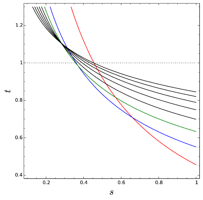
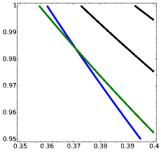
Figure 1. The curves in this plot consist of the points for which the inequalities (3.1) are attained. The region of optimality of the corner design in Example 3.4 is the region below any of the curves. On the right hand side of the picture, $|C|=3$ is the lowermost curve, then $|C|=4$, and so on. Consequently, the red, blue, green curves correspond to $|C|=3,4,5$, respectively. In the region where $s,t\leq 1$ (that is, $\beta_{A}\leq 0$), inequalities corresponding to $|C|>5$ are redundant and plotted in black. The inset shows a tiny region where the $|C|=5$ inequality is necessary. The region above the dotted line corresponds to antagonistic interaction: Two rules being active at the same time make the problem easier. In this case also inequalities for $|C|>5$ are tight.

For fixed $d$, as $k$ grows larger, more inequalities arise from Theorem 3.3. We conjecture that when $\beta_{A}<0$ for all $A$, $|A|\leq d$, as $k$ grows, a finite number of them suffices to characterize the region of optimality of $w^{*}_{k,d}$.

Conjecture 3.5.

Fix $d$ and assume all parameters have negative values: $\beta_{A}<0$, $|A|\leq d$. There exists a constant $c(d)$ such that in Theorem 3.3 the inequalities corresponding to $C$ with $|C|>c(d)$ are redundant given the remaining ones. In particular, $c(2)=5$.

Remark 3.6.

The inequalities (3.1) are restrictions on the parameters. For $d=1$ it happens that they can be rewritten as inequalities in the intensities $\lambda({\mathbf{x}},\beta)$, but in general this is not the case. In principle a semi-algebraic description in parameter space can computed. With $\phi$ the parametrization mapping coordinates $\mu$ to intensities $\lambda$, consider the set $\left\{(\mu,\lambda):\lambda=\phi(\mu),\mu\text{ satisfies \eqref{eq:cornerOpt}}\right\}$. According to the Tarski–Seidenberg theorem the projection of this semi-algebraic set to the $\lambda$ coordinates is again semi-algebraic. Actual computation, however, relies on quantifier elimination. Therefore even the best algorithms are for now unable to solve simple examples. See [3] for the theory of such computations.

We finish the discussion with a question regarding other saturated designs.

Question 3.7.

When $\beta_{A}<0$, for all $A$, $|A|\leq d$, is the corner design the only saturated design that admits $D$-optimal parameter values?

The Kiefer-Wolfowitz theorem gives a system of inequalities for any saturated design and this system characterizes parameter values for optimality. In the case $d=1,k=3$ Graßhoff et al. have shown that, up to fractional factorial designs at $\beta=0$, only the corner design yields a feasible system [10]. We have used numerical moment relaxations and semi-definite programming to numerically confirm the case $d=1,k=4$. Everything beyond this is out of reach at the moment.

3.1. Proof of Theorem 3.3

The Kiefer-Wolfowitz theorem characterizes regions of optimality of a fixed saturated design $w$ by means of inequalities in parameters $\mu_{A}$ (or equivalently $\beta_{A}$). We apply it to the corner design and make these inequalities explicit. To do so, a 0/1-matrix needs to be inverted.

Definition 3.8.

For fixed $k,d$, the model matrix $F_{k,d}$ is the matrix whose rows are the regression vectors $\{f({\mathbf{x}}):{\mathbf{x}}\in\operatorname{supp}(w^{*}_{k,d})\}$.

The rows and columns of $F_{k,d}$ may be indexed by subsets of $A\subseteq\{1,\dots,k\}$ with $|A|\leq d$ so that $F_{k,d}$ is lower triangular. We ommit the subscript indices if $k,d$ are fixed or clear from the context.

Example 3.9.

For $k=3$ and $d=2$ the model matrix is

$$F_{3,2}=\bordermatrix{&1&x_{1}&x_{2}&x_{3}&x_{1}x_{2}&x_{1}x_{3}&x_{2}x_{3}\cr 1&1&0&0&0&0&0&0\cr x_{1}&1&1&0&0&0&0&0\cr x_{2}&1&0&1&0&0&0&0\cr x_{3}&1&0&0&1&0&0&0\cr x_{1}x_{2}&1&1&1&0&1&0&0\cr x_{1}x_{3}&1&1&0&1&0&1&0\cr x_{2}x_{3}&1&0&1&1&0&0&1\cr}.$$

In the general setup of $k$ rules and interaction order $d$ the entries $F_{A,B}$ of $F$ are

$$F_{A,B}=\begin{cases}1&\text{ if }B\subseteq A\\ 0&\text{ otherwise,}\end{cases}\qquad\text{where }\,A,B\subset\{1,\dots,k\},|A|\leq d,|B|\leq d.$$

Lemma 3.10.

The inverse of $F$ has entries

$$F^{-1}_{A,B}=\begin{cases}(-1)^{|A|-|B|}&\text{ if }B\subseteq A\\ 0&\text{ otherwise.}\end{cases}$$

Proof.

Matrix multiplication yields

$$(F\cdot F^{-1})_{A,B}=\sum_{\begin{subarray}{c}C\subset\{1,\dots,k\}\\ |C|\leq d\end{subarray}}F_{A,C}F^{-1}_{C,B}=\sum_{\begin{subarray}{c}C\subset\{1,\dots,k\}\\ |C|\leq d\end{subarray}}(-1)^{|A|-|B|}\mathbbm{1}_{B\subset C}\mathbbm{1}_{C\subset A}.$$

If $A=B$, then there is only one summand, so that $(F\cdot F^{-1})_{A,A}=1$. If not, then since both matrices are lower triangular, consider the case $B\subsetneq A$ and let $a\in A\setminus B$. There is a bijection which identifies a set $C$ not containing $a$ with $C\cup\{a\}$. This bijection matches summands with opposite signs and consequently $(F\cdot F^{-1})_{A,B}=0$. ∎

If $|{\mathbf{x}}|\leq d$, then there is a row with index $B$ in $F$ that may be identified with ${\mathbf{x}}$ via $F({\mathbf{x}})_{B}=(1,{\mathbf{x}},\ldots)$. For this ${\mathbf{x}}$ we have

$$\left(F^{-T}f({\mathbf{x}})\right)_{A}=(e_{{\mathbf{x}}})_{A}:=\begin{cases}1&A=B\\ 0&\text{otherwise}.\end{cases}$$

This is a special case of the following lemma.

Lemma 3.11.

Let ${\mathbf{x}}\in\{0,1\}^{k}$ then

$$(F^{-T}f({\mathbf{x}}))_{A}=\begin{cases}(-1)^{d-|A|}\binom{|A({\mathbf{x}})|-|A|-1}{d-|A|}&\text{if }A\subset A({\mathbf{x}})\\ 0&\text{otherwise}.\end{cases}$$

Proof.

We compute

$$(F^{-T}f({\mathbf{x}}))_{A}=\sum_{|B|\leq d}(-1)^{|A|+|B|}\mathbbm{1}_{A\subset B}\mathbbm{1}_{B\subset A({\mathbf{x}})}.$$

If $A\not\subset A({\mathbf{x}})$ then all summands are zero. Therefore we can relabel the summands by sets $B^{\prime}$ disjoint from $A$ such that $B=A\cup B^{\prime}$. This yields

$$(F^{-T}f({\mathbf{x}}))_{A}=\sum_{\begin{subarray}{c}B^{\prime}\subset A({\mathbf{x}})\setminus A\\ |B^{\prime}|\leq d-|A|\end{subarray}}(-1)^{|A|+|B^{\prime}|+|A|}.$$

The result now follows from the following known formula (which is also easy to prove by induction)

$$\sum_{k=0}^{K}(-1)^{k}\binom{n}{k}=(-1)^{K}\binom{n-1}{K}.\qed$$

Proof of Theorem 3.3.

By the Kiefer-Wolfowitz theorem, a saturated design is optimal if and only if the following inequality holds for all settings ${\mathbf{x}}\in\{0,1\}^{k}$

$$\lambda({\mathbf{x}})(F^{-T}f({\mathbf{x}}))^{T}\Psi^{-1}(F^{-T}f({\mathbf{x}}))\leq 1,$$

where $\Psi=\operatorname{diag}(1,(\mu_{A})_{|A|\leq d})$. The inequalities corresponding to ${\mathbf{x}}$ with $|{\mathbf{x}}|\leq d$ are automatically satisfied with equality:

$$\lambda({\mathbf{x}})(F^{-T}f({\mathbf{x}}))^{T}\Psi^{-1}(F^{-T}f({\mathbf{x}}))=\lambda({\mathbf{x}})e_{{\mathbf{x}}}^{T}\Psi^{-1}e_{{\mathbf{x}}}=\prod_{\begin{subarray}{c}A\subset{\mathbf{x}},\\ |A|\leq d\end{subarray}}\mu_{A}\prod_{\begin{subarray}{c}A\subset{\mathbf{x}},\\ |A|\leq d\end{subarray}}\mu_{A}^{-1}=1.$$

When $|{\mathbf{x}}|\geq d+1$, using Lemma 3.11, we get the inequalities

$$\sum_{\begin{subarray}{c}B\subset A({\mathbf{x}})\\ |B|\leq d\end{subarray}}\binom{|A({\mathbf{x}})|-|B|-1}{d-|B|}^{2}\prod_{\begin{subarray}{c}A\subset A({\mathbf{x}}),|A|\leq d\\ A\neq B\end{subarray}}\mu_{A}\leq 1.\qed$$

Remark 3.12.

In the proof of Theorem 3.3, when $|{\mathbf{x}}|=d+1$, by Lemma 3.11, the entries $(F^{-T}f({\mathbf{x}}))_{A}$ are zero if $A\not\subset A({\mathbf{x}})$ and equal to $\pm 1$ if $A\subset A({\mathbf{x}})$, since in this case the binomial coefficient is $\binom{d-|A|}{d-|A|}$. We then find inequalities of the form

$$\sum_{\begin{subarray}{c}B\subset A({\mathbf{x}})\\ |B|\leq d\end{subarray}}\prod_{\begin{subarray}{c}A\subset A({\mathbf{x}}),|A|\leq d\\ A\neq B\end{subarray}}\mu_{A}\leq 1.$$

4. A geometric perspective on $D$-optimal designs

For each ${\mathbf{x}}$, the matrix $f({\mathbf{x}})f({\mathbf{x}})^{T}$ is a positive-semidefinite rank one matrix with entries zero and one. They are the vertices of the optimization domain which turns out to be a polytope:

Definition 4.1.

The information matrix polytope is

$$P(\beta)=\operatorname{conv}\left\{\lambda({\mathbf{x}},\beta)f({\mathbf{x}})f({\mathbf{x}})^{T}:{\mathbf{x}}\in\{0,1\}^{k}\right\}.$$

All points of which the convex hull is taken are also vertices of $P(\beta)$, since any affine combination of them has rank at least two. Each point in $P(\beta)$ is an information matrix $M(w,\beta)$ for some approximate design $w$. In the case $\beta=0$ (which implies $\lambda({\mathbf{x}})=1$ for all ${\mathbf{x}}$), the arising polytopes are well-known in the combinatorial optimization literature.

Example 4.2.

When $d=1$ and $\beta=0$, $P(\beta)$ is the correlation polytope. To make this obvious, one needs to omit the constant entry $1$ from the beginning of the regression function $f$. The correlation polytope is well-known in combinatorial optimization and its complexity provides lower complexity bounds there [13]. It is affinely equivalent to the even better known cut polytope via the covariance mapping [4, Chapter 5]. For higher $d$, and $\beta=0$, the polytope $P(\beta)$ is called an inclusion polytope in [11, Section 2.4.1]. It is affinely equivalent (via a generalization of the covariance mapping) to the marginal polytope of a corresponding hierararchical model.

The problem of determining an optimal experimental design has two steps

1. Determine an optimal information matrix $M^{*}$.

2. Determine weights $w$ that write the optimal matrix $M^{*}$ as a convex combination of vertices $\lambda({\mathbf{x}},\beta)f({\mathbf{x}})f({\mathbf{x}})^{T}$ of the information matrix polytope.

The possible solutions to the second problem are dealt with using convex geometry. In particular Carathéodory’s theorem applies and gives bounds for support sizes of weight vectors $w$.

In the case of $D$-optimality, the optimization problem in step 1 is to maximize the determinant over $P$. The determinant vanishes at the vertices of $P$, and since it is a log-concave function, a unique maximum with positive value is attained in the interior, as soon as there are full rank matrices in the interior. All matrices in the information matrix polytope are positive semidefinite. This motivates the linear matrix inequality (LMI) relaxation of $P(\beta)$. For this, the optimization domain $P(\beta)$ is replaced by the spectrahedron arising as the intersection of the cone of positive semidefinite matrices with the affine space spanned by $P(\beta)$.

Maximization of the determinant over a spectrahedron is a well-known convex optimization problem [20]. The unique point where the determinant is maximal is known as the analytic center of the semidefinite program. If the analytic center of the linear matrix inequality lies inside $P(\beta)$, then it gives the optimal experimental design. It is therefore an interesting problem to give a fully geometric description of the case that the analytic center lies outside of $P$.

Question 4.3.

For fixed $k,d$, as a function of $\beta$, what is the difference between $P(\beta)$ and its LMI relaxation? Through which faces can the analytic center leave $P(\beta)$ when $\beta$ changes?

Example 4.4.

Let $k=2$ and $d=1$. Setting again $\beta_{\emptyset}=0$, the two parameters of the Rasch Poisson counts model are $\lambda_{i}=e^{\beta_{i}}$, $i=1,2$. By symmetry considerations from Section 2.2 we restrict ourselves to $\beta_{i}\leq 0$, which corresponds to $\lambda_{i}\in(0,1]$. The information matrix polytope is

$$P=\operatorname{conv}\left\{\begin{pmatrix}1&0&0\\ 0&0&0\\ 0&0&0\end{pmatrix},\begin{pmatrix}\lambda_{1}&\lambda_{1}&0\\ \lambda_{1}&\lambda_{1}&0\\ 0&0&0\end{pmatrix},\begin{pmatrix}\lambda_{2}&0&\lambda_{2}\\ 0&0&0\\ \lambda_{2}&0&\lambda_{2}\end{pmatrix},\begin{pmatrix}\lambda_{1}\lambda_{2}&\lambda_{1}\lambda_{2}&\lambda_{1}\lambda_{2}\\ \lambda_{1}\lambda_{2}&\lambda_{1}\lambda_{2}&\lambda_{1}\lambda_{2}\\ \lambda_{1}\lambda_{2}&\lambda_{1}\lambda_{2}&\lambda_{1}\lambda_{2}\end{pmatrix}\right\}.$$

Independent of the values $\lambda_{1},\lambda_{2}$, the polytope $P$ is a 3-dimensional simplex. Its LMI relaxation is the intersection of the cone of $(3\times 3)$ positive-semidefinite matrices with the affine space spanned by $P$. This yields the following linear matrix inequality ($\succeq 0$ means positive-semidefinite), using the first vertex as the base point and variables $x,y,z$:

$$\left\{(x,y,z):\begin{pmatrix}1+x(\lambda_{1}-1)+y(\lambda_{2}-1)+z(\lambda_{1}\lambda_{2}-1)&\lambda_{1}x+\lambda_{1}\lambda_{2}z&\lambda_{2}y+\lambda_{1}\lambda_{2}z\\ \lambda_{1}x+\lambda_{1}\lambda_{2}z&\lambda_{1}x+\lambda_{1}\lambda_{2}z&\lambda_{1}\lambda_{2}z\\ \lambda_{2}y+\lambda_{1}\lambda_{2}z&\lambda_{1}\lambda_{2}z&\lambda_{2}y+\lambda_{1}\lambda_{2}z\end{pmatrix}\succeq 0\right\}.$$

Figure 2 contains plots of the resulting spectrahedra “along the diagonal” $\lambda:=\lambda_{1}=\lambda_{2}$.

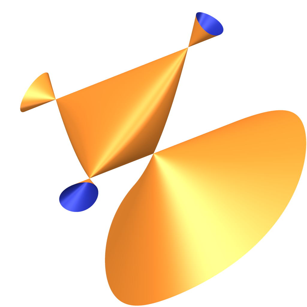
Figure 2. Vanishing surfaces of the determinant in Example 4.4. In each plot, the bounded region is the spectrahedron. As the parameter moves from $\lambda=1$ (left) through $\lambda=0.45$ (middle) to $\lambda=0.2$ (right) it elongates. The ear-shaped cones emerging from the vertices do not touch in the left-most picture. As soon as $\lambda<1$, they do touch: Even in the middle picture, the cone going off to the bottom and the sheet emerging from the three remaining vertices are connected in codimension one (outside of the pictured area). If $\lambda_{1}=1$, but $\lambda_{2}<1$, then exactly three of the four vertex cones meet eventually.

Each of the three spectrahedra has four vertices, although this is hardly visible in the rightmost picture. These are also the vertices of $P$. In fact, when $\lambda$ is close to 1, the spectrahedron looks like a bloated version of $P$. The analytic center of the LMI is the point $(x,y,z)$ where the determinant is maximal. Numerical approximations can be computed efficiently with semidefinite optimization (we used yalmip [16] in Matlab). Some values are given in Table 1.

$\lambda$	analytic center
1	$(0.250,0.250,0.250)$
0.8	$(0.254,0.254,0.217)$
0.5	$(0.300,0.300,0.094)$
$\sqrt{2}-1$	$(0.333,0.333,0.000)$
0.4	$(0.343,0.343,-0.023)$
0.2	$(1.580,1.580,-2.976)$

Table 1. Coordinates of the analytic center as a function of $\lambda$.

Interestingly, the mosek solver that we used declares the spectrahedron as unbounded for parameter values $\lambda<0.171$. The transition of the $D$-optimal design to a saturated design at $\sqrt{2}-1$ found in [8] is visible here as the analytic center leaves the polytope $P$ at that parameter value. In this sense, the optimality of certain designs can be understood in terms of the geometry of deforming spectrahedra.

We close by mentioning another connection between polyhedral and spectrahedral geometry. The elliptope is the spectrahedron consisting of all positive semi-definite matrices with entries one on the diagonal (so-called correlation matrices). It is a well-known relaxation of the correlation polytope and its polyhedral faces have received considerable attention (see [14, 15]). Example 4.4 motivates the study of the deformation of the linear matrix inequalities arising from affine hulls of information polytopes. Each such deformation starts at an elliptope when $\beta=0$. As $\beta$ becomes more negative, the spectrahedron deforms and eventually its analytic center leaves the information matrix polytope. A thorough understanding of this phenomenon would probably yield new insights about optimality of experimental designs, in particular Question 3.7.

References

- [1] 4ti2 team, 4ti2—A software package for algebraic, geometric and combinatorial problems on linear spaces, available at www.4ti2.de, 2007.
- [2] Satoshi Aoki, Hisayuki Hara, and Akimichi Takemura, Markov bases in algebraic statistics, vol. 199, Springer Science & Business Media, 2012.
- [3] Saugata Basu, Richard D Pollack, and Marie-Françoise Roy, Algorithms in real algebraic geometry, vol. 10, Springer, 2006.
- [4] M.M. Deza and Monique Laurent, Geometry of cuts and metrics, Algorithms and Combinatorics, Springer, Berlin, 1997.
- [5] Persi Diaconis and Bernd Sturmfels, Algebraic algorithms for sampling from conditional distributions, Annals of Statistics 26 (1998), 363–397.
- [6] Anna Doebler and Heinz Holling, A processing speed test based on rule-based item generation: An analysis with the Rasch Poisson counts model, Learning and Individual Differences (2015).
- [7] Mathias Drton, Bernd Sturmfels, and Seth Sullivant, Lectures on algebraic statistics, Oberwolfach Seminars, vol. 39, Springer, Berlin, 2009, A Birkhäuser book.
- [8] Ulrike Graßhoff, Heinz Holling, and Rainer Schwabe, Optimal design for count data with binary predictors in item response theory, Advances in Model-Oriented Design and Analysis, Springer, 2013, pp. 117–124.
- [9] by same author, Optimal design for the Rasch Poisson counts model with multiple binary predictors, Tech. report, 2014.
- [10] by same author, Poisson model with three binary predictors: When are saturated designs optimal?, Stochastic Models, Statistics and Their Applications (Ansgar Steland, Ewaryst Rafajłowicz, and Krzysztof Szajowski, eds.), 2015, pp. 75–81.
- [11] Thomas Kahle, On boundaries of statistical models, Ph.D. thesis, Leipzig University, 2010.
- [12] Thomas Kahle, Eckehard Olbrich, Jürgen Jost, and Nihat Ay, Complexity measures from interaction structures, Physical Review E 79 (2009), 026201.
- [13] Volker Kaibel and Stefan Weltge, A short proof that the extension complexity of the correlation polytope grows exponentially, Discrete & Computational Geometry 53 (2013), no. 2, 397–401.
- [14] Monique Laurent and Svatopluk Poljak, On a positive semidefinite relaxation of the cut polytope, Linear Algebra and its Applications 223 (1995), 439–461.
- [15] by same author, On the facial structure of the set of correlation matrices, SIAM Journal on Matrix Analysis and Applications 17 (1996), no. 3, 530–547.
- [16] J. Löfberg, YALMIP: A toolbox for modeling and optimization in MATLAB, Proceedings of the CACSD Conference (Taipei, Taiwan), 2004.
- [17] Friedrich Pukelsheim, Optimal design of experiments, Classics in Applied Mathematics, vol. 50, SIAM, 2006.
- [18] Martin Radloff and Rainer Schwabe, Invariance and equivariance in experimental design for nonlinear models, preprint (2015).
- [19] Bernd Sturmfels, Gröbner bases and convex polytopes, University Lecture Series, vol. 8, American Mathematical Society, Providence, RI, 1996.
- [20] Lieven Vandenberghe and Stephen Boyd, Semidefinite programming, SIAM Review 38 (1996), no. 1, 49–95.