Finding optimal solutions for generalized quantum state discrimination problems

Abstract

We try to find an optimal quantum measurement for generalized quantum state discrimination problems, which include the problem of finding an optimal measurement maximizing the average correct probability with and without a fixed rate of inconclusive results and the problem of finding an optimal measurement in the Neyman-Pearson strategy. We propose an approach in which the optimal measurement is obtained by solving a modified version of the original problem. In particular, the modified problem can be reduced to one of finding a minimum error measurement for a certain state set, which is relatively easy to solve. We clarify the relationship between optimal solutions to the original and modified problems, with which one can obtain an optimal solution to the original problem in some cases. Moreover, as an example of application of our approach, we present an algorithm for numerically obtaining optimal solutions to generalized quantum state discrimination problems.

I Introduction

A fundamental issue in quantum mechanics is that there is no way to discriminate perfectly between non-orthogonal quantum states, and indeed discrimination between quantum states has become a crucial task in quantum information theory. The object of this task is to distinguish between a given finite set of known quantum states with given prior probabilities as well as possible. This task can be viewed as finding a quantum measurement that minimizes or maximizes a certain optimality criterion. Several optimality criteria have been suggested since the basic framework of quantum state discrimination was established by the pioneering work of Helstrom, Holevo, and Yuen et al. Holevo (1973); Helstrom (1976); Yuen et al. (1975).

A minimum error measurement is one that maximizes the average correct probability, and it is the most intensively investigated. In particular, necessary and sufficient conditions for a minimum error measurement have been formulated Holevo (1973); Helstrom (1976); Yuen et al. (1975); Eldar et al. (2003), and closed-form analytical expressions have been derived for some classes of quantum state sets (see e.g., Belavkin (1975); Ban et al. (1997); Usuda et al. (1999); Eldar and Forney Jr. (2001)). Another kind of measurement, called unambiguous measurement, achieves error-free, i.e., unambiguous, discrimination at the expense of allowing for a certain rate of inconclusive answers Ivanovic (1987); Dieks (1988); Peres (1988). An unambiguous measurement that maximizes the average correct probability is called optimal, and a closed-form analytical expression has been obtained for some cases (see, e.g., Eldar (2003a); Herzog (2007); Pang and Wu (2009); Kleinmann et al. (2010); Roa et al. (2011); Bergou et al. (2012); Bandyopadhyay (2014)).

In addition to the minimum error and optimal unambiguous measurements, several other kinds of quantum measurements have been studied; for example, an optimal inconclusive measurement Chefles and Barnett (1998); Eldar (2003b); Fiurášek and Ježek (2003); Herzog (2012); Nakahira et al. (2012); Bagan et al. (2012); Herzog (2015), an optimal error margin measurement Touzel et al. (2007); Hayashi et al. (2008); Sugimoto et al. (2009), and an optimal measurement in the Neyman-Pearson strategy Helstrom (1976); Holevo (1982); Paris (1997). Recently, generalized quantum state discrimination problems, which include any problems related to finding any of the optimal measurements described above, have been investigated, and necessary and sufficient conditions for an optimal measurement have also been formulated Nakahira et al. (2015a). However, thus far, obtaining a closed-form analytical expression appears to be a very difficult task. Moreover, an efficient numerical algorithm for solving such problems has not yet been found.

In this article, we try to find analytical or numerical optimal solutions to generalized quantum state discrimination problems. We consider an extension of the method developed in Ref. Nakahira et al. (2015b). The authors of that paper developed a corresponding modified version of an optimal inconclusive measurement that maximizes an objective function which is the weighted sum of the average correct and inconclusive probabilities. In this paper, we investigate a modified version of a generalized problem. As we will show later, finding an optimal solution to the modified problem is relatively easy, since it can be reduced to one of finding a minimum error measurement for a certain state set. Thus, the modified problem is often useful for solving the original generalized problem. In Sec. II, we give a brief overview of generalized quantum state discrimination problems. In Sec. III, we present the corresponding modified problem and clarify the relationship between optimal solutions to the original and modified problems. We also claim that in the two-dimensional cases one can obtain an optimal solution to the original problem from the solution to the modified problem. In Sec. IV, we propose a numerical algorithm for solving the original problem by exploiting the modified one.

II Generalized quantum state discrimination problem

A quantum measurement can be described as a positive operator-valued measure (POVM) with $M$ detection operators, $\Pi=\{\hat{\Pi}_{m}:m\in\mathcal{I}_{M}\}$, where $\mathcal{I}_{k}=\{0,1,\cdots,k-1\}$. Let $\mathcal{H}$ be a complex Hilbert space and $\mathcal{M}_{M}$ be the set of POVMs on $\mathcal{H}$ whose element consists of $M$ detection operators. Each $\Pi\in\mathcal{M}_{M}$ satisfies

$$\hat{\Pi}_{m} \geq 0,~{}~{}~{}\forall m\in\mathcal{I}_{M},$$

$$\sum_{m=0}^{M-1}\hat{\Pi}_{m} = \hat{1},$$ (1)

where $\hat{1}$ is the identity operator on $\mathcal{H}$. $\hat{A}\geq 0$ and $\hat{A}\geq\hat{B}$ respectively denote that $\hat{A}$ and $\hat{A}-\hat{B}$ are positive semidefinite.

Let $\mathcal{S}$ and $\mathcal{S}_{+}$ be respectively the sets of Hermitian operators on $\mathcal{H}$ and semidefinite positive operators on $\mathcal{H}$. Let $\mathbf{R}$ and $\mathbf{R}_{+}$ be respectively the sets of real numbers and nonnegative real numbers. Also, let $\mathbf{R}^{n}$ and $\mathbf{R}_{+}^{n}$ be respectively the sets of collections of $n$ real numbers and $n$ nonnegative real numbers.

A broad class of optimization problems regarding quantum measurements, including ones of finding a minimum error measurement and an optimal unambiguous measurement, can be formulated as follows Nakahira et al. (2015a):

$$\begin{array}[]{lll}{\rm P1:}&{\rm maximize}&\displaystyle f(\Pi)=\sum_{m=0}^{M-1}{\rm Tr}(\hat{c}_{m}\hat{\Pi}_{m})\\ &{\rm subject~{}to}&\Pi\in\mathcal{M}_{M}^{(b)},\\ \end{array}$$ (4)

where $\hat{c}_{m}\in\mathcal{S}$ for any $m\in\mathcal{I}_{M}$. $\mathcal{M}_{M}^{(b)}$ with $b=\{b_{j}\in\mathbf{R}:j\in\mathcal{I}_{J}\}\in\mathbf{R}^{J}$ is defined as:

$$\mathcal{M}_{M}^{(b)} = \left\{\Pi\in\mathcal{M}_{M}:\beta_{j}(\Pi)\geq b_{j},~{}\forall j\in\mathcal{I}_{J}\right\},$$

$$\beta_{j}(\Pi) = \sum_{m=0}^{M-1}{\rm Tr}(\hat{a}_{j,m}\hat{\Pi}_{m}),$$ (5)

where $\hat{a}_{j,m}\in\mathcal{S}$ $~{}(\forall j\in\mathcal{I}_{J},m\in\mathcal{I}_{M})$, and $J$ is the number of constraints expressed in the form $\beta_{j}(\Pi)\geq b_{j}$. Problem P1 is referred to as a generalized quantum state discrimination problem. Without loss of generality, we will let $\mathcal{H}$ be the complex Hilbert space spanned by the supports of the operators $\{\hat{c}_{m}:m\in\mathcal{I}_{M}\}$ and $\{\hat{a}_{j,m}:j\in\mathcal{I}_{J},m\in\mathcal{I}_{M}\}$. Note that to simplify the discussion, we have reversed the sign of the inequality in Eq. (5) with respect to that in Ref. Nakahira et al. (2015a). A POVM $\Pi$ that satisfies the constraints is referred to as a feasible solution. Moreover, the set of all feasible solutions is called a feasible set. The feasible set of problem P1 is $\mathcal{M}_{M}^{(b)}$.

As an example, let us consider the problem of finding a minimum error measurement. Suppose we want to discriminate between $R$ quantum states represented by density operators $\hat{\rho}_{r}$ $~{}(r\in\mathcal{I}_{R})$ with prior probabilities $\xi_{r}$. $\hat{\rho}_{r}$ satisfies $\hat{\rho}_{r}\geq 0$ and ${\rm Tr}~{}\hat{\rho}_{r}=1$. A minimum error measurement $\Pi\in\mathcal{M}_{R}$ for $R$ quantum states $\rho=\{\hat{\rho}_{r}:r\in\mathcal{I}_{R}\}$ with prior probabilities $\xi=\{\xi_{r}:r\in\mathcal{I}_{R}\}$ can be characterized as an optimal solution to the following optimization problem:

$$\begin{array}[]{ll}{\rm maximize}&\displaystyle P_{\rm C}(\Pi)=\sum_{r=0}^{R-1}\xi_{r}{\rm Tr}(\hat{\rho}_{r}\hat{\Pi}_{r})\\ {\rm subject~{}to}&\Pi\in\mathcal{M}_{R}.\\ \end{array}$$ (8)

$P_{\rm C}(\Pi)$ is called the average correct probability. This problem is equivalent to problem P1 with $M=R$, $J=0$, and $\hat{c}_{m}=\xi_{m}\hat{\rho}_{m}$ $~{}(m\in\mathcal{I}_{R})$.

In the remainder of this paper, we assume that $\hat{c}_{m}\in\mathcal{S}_{+}$ and $\hat{a}_{j,m}\in\mathcal{S}_{+}$ for any $j\in\mathcal{I}_{J}$ and $m\in\mathcal{I}_{M}$. We show here that this involves no loss of generality. For given $\{\hat{c}_{m}\in\mathcal{S}:m\in\mathcal{I}_{M}\}$, we choose $\hat{\tau}_{\rm c}\in\mathcal{S}$ such that $\hat{c}_{m}+\hat{\tau}_{\rm c}\geq 0$. Similarly, for given $\{\hat{a}_{j,m}\in\mathcal{S}:m\in\mathcal{I}_{M}\}$, we choose $\hat{\tau}_{j}\in\mathcal{S}$ such that $\hat{a}_{j,m}+\hat{\tau}_{j}\geq 0$. Let

$$\hat{c}^{\prime}_{m} = \hat{c}_{m}+\hat{\tau}_{\rm c},$$

$$\hat{a}^{\prime}_{j,m} = \hat{a}_{j,m}+\hat{\tau}_{j};$$ (9)

$\hat{c}^{\prime}_{m}\geq 0$ and $\hat{a}^{\prime}_{j,m}\geq 0$ obviously hold. We have

$$\sum_{m=0}^{M-1}{\rm Tr}(\hat{c}^{\prime}_{m}\hat{\Pi}_{m}) = \sum_{m=0}^{M-1}{\rm Tr}(\hat{c}_{m}\hat{\Pi}_{m})+{\rm Tr}~{}\hat{\tau}_{\rm c},$$

$$\sum_{m=0}^{M-1}{\rm Tr}(\hat{a}^{\prime}_{j,m}\hat{\Pi}_{m}) = \sum_{m=0}^{M-1}{\rm Tr}(\hat{a}_{j,m}\hat{\Pi}_{m})+{\rm Tr}~{}\hat{\tau}_{j}.$$ (10)

Thus, we can easily see that an optimal solution to problem P1 does not change even if we replace $\hat{c}^{\prime}_{m}$, $\hat{a}^{\prime}_{j,m}$, and $b_{j}+{\rm Tr}~{}\hat{\tau}_{j}$ with $\hat{c}_{m}$, $\hat{a}_{j,m}$, and $b_{j}$, respectively.

Let $f^{\star}(b)$ be the optimal value of problem P1 as a function of $b\in\mathbf{R}^{J}$ if $\mathcal{M}_{M}^{(b)}$ is not empty; otherwise, $f^{\star}(b)=-\infty$. $f^{\star}(b)$ can be expressed as

$$f^{\star}(b) = \left\{\begin{array}[]{ll}\displaystyle\max_{\Pi\in\mathcal{M}_{M}^{(b)}}f(\Pi),\\ -\infty,&~{}{\rm otherwise}.\end{array}\right.$$ (13)

We can easily verify that if $b,b^{\prime}\in\mathbf{R}^{J}$ satisfies $b_{j}\leq b^{\prime}_{j}$ for any $j\in\mathcal{I}_{J}$, then $\mathcal{M}_{M}^{(b)}\supseteq\mathcal{M}_{M}^{(b^{\prime})}$ holds, which gives $f^{\star}(b)\geq f^{\star}(b^{\prime})$. In addition, since ${\rm Tr}(\hat{a}_{j,m}\hat{\Pi}_{m})\geq 0$ always holds, the problem is equivalent to that in which $b_{j}$ with $b_{j}<0$ is replaced with 0; thus, for any $b\in\mathbf{R}^{J}$, $f^{\star}(b)=f^{\star}(b^{\prime})$ holds, where $b^{\prime}\in\mathbf{R}_{+}^{J}$ satisfies $b^{\prime}_{j}=\max(b_{j},0)$ for any $j\in\mathcal{I}_{J}$.

The dual problem of problem P1 can be expressed as Nakahira et al. (2015a)

$$\begin{array}[]{lll}{\rm DP1:}&{\rm minimize}&\displaystyle s(\hat{X},\lambda)={\rm Tr}~{}\hat{X}-\lambda\cdot b\\ &{\rm subject~{}to}&\hat{X}\in\mathcal{S}_{\lambda}\\ \end{array}$$ (16)

with variables $\hat{X}\in\mathcal{S}_{+}$ and $\lambda=\{\lambda_{j}\in\mathbf{R}_{+}:j\in\mathcal{I}_{J}\}\in\mathbf{R}_{+}^{J}$, where $\lambda\cdot b$ denotes $\sum_{j=0}^{J-1}\lambda_{j}b_{j}$ and

$$\mathcal{S}_{\lambda} = \{\hat{X}\in\mathcal{S}_{+}:\hat{X}\geq\hat{z}_{m}(\lambda),~{}\forall m\in\mathcal{I}_{M}\},$$ (17)

$$\hat{z}_{m}(\lambda) = \hat{c}_{m}+\sum_{j=0}^{J-1}\lambda_{j}\hat{a}_{j,m}.$$ (18)

$\hat{z}_{m}(\lambda)\in\mathcal{S}_{+}$ obviously holds for any $\lambda\in\mathbf{R}_{+}^{J}$ since $\hat{c}_{m}\geq 0$ and $\hat{a}_{j,m}\geq 0$. If $\mathcal{M}_{M}^{(b)}$ is not empty, then the optimal values of problems P1 and D1 are the same (see Ref. Nakahira et al. (2015a) Theorem 1).

III Modified version of generalized quantum state discrimination problem

Necessary and sufficient conditions have been formulated for an optimal solution (i.e., a minimum error measurement) to problem (8), and closed-form analytical expressions for minimum error measurements have also been derived for several quantum state sets. Similarly, necessary and sufficient conditions have been derived for an optimal solution to problem P1 Nakahira et al. (2015a). However, obtaining an optimal solution to problem P1 is often a more difficult task than obtaining a minimum error measurement. In this section, we consider a modified optimization problem. We claim that, in some cases, solving the modified problem is easier than directly solving problem P1.

III.1 Formulation

The main reason why it is difficult to obtain an analytic solution to problem P1 in general is that the constraints are more complicated than those of finding a minimum error measurement. Let us consider the following problem:

$$\begin{array}[]{lll}{\rm P2:}&{\rm maximize}&\displaystyle g(\Pi;\lambda)=\sum_{m=0}^{M-1}{\rm Tr}[\hat{z}_{m}(\lambda)\hat{\Pi}_{m}]\\ &{\rm subject~{}to}&\Pi\in\mathcal{M}_{M},\\ \end{array}$$ (21)

where $\lambda\in\mathbf{R}_{+}^{J}$ is constant, and $\hat{z}_{m}(\lambda)$ is defined in Eq. (18). We call this problem the modified problem of problem P1. We can easily see that it can also be formulated as a generalized quantum state discrimination problem Nakahira et al. (2015a), and thus the dual problem is expressed as

$$\begin{array}[]{lll}{\rm DP2:}&{\rm minimize}&\displaystyle{\rm Tr}~{}\hat{X}\\ &{\rm subject~{}to}&\hat{X}\in\mathcal{S}_{\lambda}\\ \end{array}$$ (24)

with variables $\hat{X}\in\mathcal{S}_{+}$. The optimal values of problems P2 and DP2 are the same. Let $g^{\star}(\lambda)$ be the function of $\lambda\in\mathbf{R}^{J}$ defined by

$$g^{\star}(\lambda) = \left\{\begin{array}[]{ll}\displaystyle\max_{\Pi\in\mathcal{M}_{M}}g(\Pi;\lambda),&~{}\lambda\in\mathbf{R}_{+}^{J},\\ \infty,&~{}{\rm otherwise};\end{array}\right.$$ (27)

i.e., $g^{\star}(\lambda)$ is the optimal value of problem P2 in the case of $\lambda\in\mathbf{R}_{+}^{J}$; otherwise, $\infty$. If $\lambda,\lambda^{\prime}\in\mathbf{R}_{+}^{J}$ satisfies $\lambda_{j}\geq\lambda^{\prime}_{j}$ for any $j\in\mathcal{I}_{J}$, then $\hat{z}_{m}(\lambda)\geq\hat{z}_{m}(\lambda^{\prime})$ holds for any $m\in\mathcal{I}_{M}$, and thus $g^{\star}(\lambda)\geq g^{\star}(\lambda^{\prime})$ holds.

III.2 Relationship between problems P1 and P2

In this subsection, we discuss the relationship between problems P1 and P2. First, we show that $f^{\star}(b)$ and $g^{\star}(\lambda)$ have the following property:

Theorem 1

$-f^{\star}(b)$ and $g^{\star}(\lambda)$ are convex. Moreover, $-f^{\star}(b)$ is the Legendre transformation of $g^{\star}(\lambda)$ and vice versa.

Proof

First, we prove that $g^{\star}(\lambda)$ is convex. From Eq. (27), it suffices to show that $g^{\star}(\lambda)$ is convex in the range of $\lambda\in\mathbf{R}_{+}^{J}$. Let $\hat{X}^{\prime}$ and $\hat{X}^{\prime\prime}$ be respectively optimal solutions to problem DP2 in the case of $\lambda=\lambda^{\prime}\in\mathbf{R}_{+}^{J}$ and $\lambda=\lambda^{\prime\prime}\in\mathbf{R}_{+}^{J}$, which means that $g^{\star}(\lambda^{\prime})={\rm Tr}~{}\hat{X}^{\prime}$, $\hat{X}^{\prime}\in\mathcal{S}_{\lambda^{\prime}}$, $g^{\star}(\lambda^{\prime\prime})={\rm Tr}~{}\hat{X}^{\prime\prime}$, and $\hat{X}^{\prime\prime}\in\mathcal{S}_{\lambda^{\prime\prime}}$ hold. Let $t\in\mathbf{R}_{+}$ with $0\leq t\leq 1$, $\hat{Y}=t\hat{X}^{\prime}+(1-t)\hat{X}^{\prime\prime}$, and $\eta=\{\eta_{j}=t\lambda^{\prime}_{j}+(1-t)\lambda^{\prime\prime}_{j}:j\in\mathcal{I}_{J}\}$. $\eta\in\mathbf{R}_{+}^{J}$ obviously holds. For any $m\in\mathcal{I}_{M}$, we have

$$\hat{Y} = t\hat{X}^{\prime}+(1-t)\hat{X}^{\prime\prime}$$ (28)

$$\geq t\hat{z}_{m}(\lambda^{\prime})+(1-t)\hat{z}_{m}(\lambda^{\prime\prime})=\hat{z}_{m}(\eta);$$

i.e., $\hat{Y}\in\mathcal{S}_{\eta}$. The last equality of Eq. (28) follows from the definition of $\hat{z}_{m}(\lambda)$ in Eq. (18). Thus, $g^{\star}(\eta)\leq{\rm Tr}~{}\hat{Y}$ holds from the definition of $g^{\star}(\eta)$. Therefore, we obtain

$$g^{\star}(\eta) \leq {\rm Tr}~{}\hat{Y}=t{\rm Tr}~{}\hat{X}^{\prime}+(1-t){\rm Tr}~{}\hat{X}^{\prime\prime}$$ (29)

$$= tg^{\star}(\lambda^{\prime})+(1-t)g^{\star}(\lambda^{\prime\prime}),$$

which indicates that $g^{\star}(\lambda)$ is convex.

Next, we prove that $-f^{\star}(b)$ is the Legendre transformation of $g^{\star}(\lambda)$. Let $\hat{X}_{\lambda}$ be an optimal solution to problem DP2 as a function of $\lambda\in\mathbf{R}_{+}^{J}$. $g^{\star}(\lambda)={\rm Tr}~{}\hat{X}_{\lambda}$ holds in the case of $\lambda\in\mathbf{R}_{+}^{J}$. Since the minimum $s(\hat{X},\lambda)$ in Eq. (16) equals the optimal value $f^{\star}(b)$ of problem P1, we obtain

$$-f^{\star}(b) = -\min_{\lambda\in\mathbf{R}_{+}^{J}}\min_{\hat{X}\in\mathcal{S}_{\lambda}}({\rm Tr}~{}\hat{X}-\lambda\cdot b)$$ (30)

$$= -\min_{\lambda\in\mathbf{R}_{+}^{J}}({\rm Tr}~{}\hat{X}_{\lambda}-\lambda\cdot b)$$

$$= -\min_{\lambda\in\mathbf{R}_{+}^{J}}\left[g^{\star}(\lambda)-\lambda\cdot b\right]$$

$$= \max_{\lambda\in\mathbf{R}^{J}}\left[\lambda\cdot b-g^{\star}(\lambda)\right],$$

where the second line follows from $\min_{\hat{X}\in\mathcal{S}_{\lambda}}{\rm Tr}~{}\hat{X}={\rm Tr}~{}\hat{X}_{\lambda}$, which is given by the definition of $\hat{X}_{\lambda}$. From Eq. (30), $-f^{\star}(b)$ is the Legendre transformation of $g^{\star}(\lambda)$.

We can obviously see that $-f^{\star}(b)$ is convex and $g^{\star}(\lambda)$ is the Legendre transformation of $-f^{\star}(b)$ since $-f^{\star}(b)$ is the Legendre transformation of the convex function $g^{\star}(\lambda)$ Hiriart-Urruty and Lemaréchal (2001). $\blacksquare$

Next, we discuss the relationship between optimal solutions to problems P1 and P2.

Theorem 2

The following statements hold:

1. An optimal solution to problem P1 with respect to $b\in\mathbf{R}^{J}$ is an optimal solution to problem P2 with respect to $\lambda\in\partial[-f^{\star}(b)]$, where $\partial[-f^{\star}(b)]$ is the subdifferential of $-f^{\star}(b)$, i.e.,

   $$\partial[-f^{\star}(b)] = \{\lambda\in\mathbf{R}_{+}^{J}:-f^{\star}(b^{\prime})+f^{\star}(b)$$ (31)

   $$~{}~{}\geq\lambda\cdot b^{\prime}-\lambda\cdot b,~{}\forall b^{\prime}\in\mathbf{R}^{J}\}.$$

2. An optimal solution, denoted by $\Pi^{\bullet}$, to problem P2 with respect to $\lambda\in\mathbf{R}_{+}^{J}$ is an optimal solution to problem P1 with respect to $b\in\mathbf{R}^{J}$ if

   $$\beta_{j}(\Pi^{\bullet}) \geq b_{j},$$

   $$\lambda_{j}[\beta_{j}(\Pi^{\bullet})-b_{j}] = 0$$ (32)

   hold for any $j\in\mathcal{I}_{J}$ (note that $\beta_{j}$ is defined by Eq. (5)).

Proof

(1) Let $\Pi^{\star}$ be an optimal solution to problem P1 with respect to $b\in\mathbf{R}^{J}$. For any $\lambda\in\partial[-f^{\star}(b)]$, we have

$$g^{\star}(\lambda) = \max_{b^{\prime}\in\mathbf{R}^{J}}[\lambda\cdot b^{\prime}+f^{\star}(b^{\prime})]$$ (33)

$$= \lambda\cdot b+f^{\star}(b)$$

$$= \lambda\cdot b+\sum_{m=0}^{M-1}{\rm Tr}(\hat{c}_{m}\hat{\Pi}_{m}^{\star})$$

$$\leq \sum_{m=0}^{M-1}{\rm Tr}[\hat{z}_{m}(\lambda)\hat{\Pi}_{m}^{\star}]$$

$$= g(\Pi^{\star};\lambda),$$

where the first line follows from $g^{\star}(\lambda)$ being the Legendre transformation of $-f^{\star}(b)$. The second line follows from $\lambda\cdot b+f^{\star}(b)\geq\lambda\cdot b^{\prime}+f^{\star}(b^{\prime})$ for any $b^{\prime}\in\mathbf{R}^{J}$, which is given from Eq. (31). The fourth line follows from $\Pi^{\star}\in\mathcal{M}_{M}^{(b)}$ (i.e., $\beta_{j}(\Pi^{\star})\geq b_{j},~{}\forall j\in\mathcal{I}_{J}$) and Eq. (18). In contrast, from the definition of $g^{\star}(\lambda)$, $g^{\star}(\lambda)\geq g(\Pi^{\star};\lambda)$ holds. Thus, $g^{\star}(\lambda)=g(\Pi^{\star};\lambda)$ holds, which means that $\Pi^{\star}$ is an optimal solution to problem P2.

(2) Let us consider $b$ satisfying Eq. (32). Suppose, by contradiction, that $\Pi^{\bullet}$ is not an optimal solution to problem P1 with respect to $b$. Since $\beta_{j}(\Pi^{\bullet})\geq b_{j}$ holds for any $j\in\mathcal{I}_{J}$, $\Pi^{\bullet}\in\mathcal{M}_{M}^{(b)}$ holds. Let $\Pi^{\prime}$ be an optimal solution to problem P1 with respect to $b$; then, $\Pi^{\prime}\in\mathcal{M}_{M}^{(b)}$ and $f(\Pi^{\prime})>f(\Pi^{\bullet})$ hold. Thus, we obtain

$$g(\Pi^{\prime};\lambda) = f(\Pi^{\prime})+\sum_{j=0}^{J-1}\lambda_{j}\beta_{j}(\Pi^{\prime})$$ (34)

$$> f(\Pi^{\bullet})+\sum_{j=0}^{J-1}\lambda_{j}b_{j}$$

$$= f(\Pi^{\bullet})+\sum_{j=0}^{J-1}\lambda_{j}\beta_{j}(\Pi^{\bullet})$$

$$= g(\Pi^{\bullet};\lambda).$$

This contradicts the assumption that $\Pi^{\bullet}$ is an optimal solution to problem P2 with respect to $\lambda$, i.e., $g(\Pi^{\bullet};\lambda)\geq g(\Pi^{\prime};\lambda)$ for any $\Pi^{\prime}\in\mathcal{M}_{M}$. Therefore, $\Pi^{\bullet}$ is an optimal solution to problem P1 with respect to $b$. $\blacksquare$

III.3 Derivation of an optimal solution using modified problem

As we will show below, problem P2 can be reduced to one of finding a minimum error measurement for a certain state set. Thus, sometimes, problem P2 can be used to solve problem P1 and is easier than directly solving it.

Remark 3

Let us consider problem P2 with respect to $\lambda\in\mathbf{R}_{+}^{J}$. $\Pi\in\mathcal{M}_{M}$ is an optimal solution to problem P2 if and only if $\Pi$ is a minimum error measurement for $M$ quantum states $\rho=\{\hat{\rho}_{m}:m\in\mathcal{I}_{M}\}$ with prior probabilities $\xi=\{\xi_{m}:m\in\mathcal{I}_{M}\}$, where

$$\xi_{m} = \frac{{\rm Tr}~{}\hat{z}_{m}(\lambda)}{\displaystyle\sum_{k=0}^{M-1}{\rm Tr}~{}\hat{z}_{k}(\lambda)},~{}~{}~{}\hat{\rho}_{m}=\frac{\hat{z}_{m}(\lambda)}{{\rm Tr}~{}\hat{z}_{m}(\lambda)}.$$ (35)

Proof

Let $C=[\sum_{k=0}^{M-1}{\rm Tr}~{}\hat{z}_{k}(\lambda)]^{-1}$. The average correct probability $P_{\rm C}(\Pi)$, which is defined by Eq. (8), can be represented as

$$P_{\rm C}(\Pi) = \sum_{m=0}^{M-1}\xi_{m}{\rm Tr}(\hat{\rho}_{m}\hat{\Pi}_{m})$$ (36)

$$= C\sum_{m=0}^{M-1}{\rm Tr}[\hat{z}_{m}(\lambda)\hat{\Pi}_{m}]=Cg(\Pi;\lambda).$$

Thus, finding a $\Pi$ that maximizes $P_{\rm C}(\Pi)$ is equivalent to finding a $\Pi$ that maximizes $g(\Pi;\lambda)$. $\blacksquare$

Closed-form analytical expressions of minimum error measurements have been obtained for several classes of quantum state sets (e.g., Belavkin (1975); Ban et al. (1997); Usuda et al. (1999); Eldar and Forney Jr. (2001); Usuda et al. (2002); Andersson et al. (2002); Eldar et al. (2004); Herzog (2004); Deconinck and Terhal (2010)). By using these results, we should be able to obtain a closed-form analytical expression for problem P1 in some cases. For example, an analytical procedure for finding a minimum error measurement for any qubit state set is shown in Ref. Deconinck and Terhal (2010). This method is applicable to problem P1 with $\dim~{}\mathcal{H}=2$ since the corresponding modified problem can be reduced to one of finding a minimum error measurement for a qubit state set. The optimal value and solution of problem P1 can be derived from Theorems 1 and 2 once we find those of the corresponding modified problem.

IV Numerical algorithm for solving a generalized quantum state discrimination problem

In this section, we present a numerical algorithm of solving a generalized quantum state discrimination problem by utilizing the modified one. Problem P1 can be formulated as a semidefinite programming (SDP) problem; thus, in general, an optimal solution can be computed in polynomial time in $N=\dim~{}\mathcal{H}$ by using well known algorithms such as interior point methods. However, these methods require excessive computational resources when $N$ is very large (e.g., Zibulevsky and Elad (2010)). For example, the time complexity required by CSDP (which is a widely used SDP solver implementing a primal-dual interior point method) is $O(N^{6})$.

Ježek et al. proposed an iterative algorithm for obtaining a minimum error measurement, which we call Ježek et al.’s algorithm Ježek et al. (2002). Later, Fiurášek et al. extended this algorithm to an optimal inconclusive measurement Fiurášek and Ježek (2003). These algorithms resemble projected gradient-based algorithms, which consist of a gradient step (i.e., approaching the optimal value of the objective function) and a projection step (i.e., projecting a solution onto the feasible set). However, the projection onto the feasible set is computationally expensive even for moderately complex constraints. We propose a low computational complexity numerical algorithm for solving problem P1 that works by solving modified problem P2 and does not always project a solution onto the feasible set of problem P1 at each iteration.

IV.1 Conventional method

Let us explain Ježek et al.’s algorithm Ježek et al. (2002). Consider a quantum state set $\{\hat{\rho}_{r}:r\in\mathcal{I}_{R}\}$ with prior probabilities $\{\xi_{r}:r\in\mathcal{I}_{R}\}$. This algorithm iteratively computes $\Pi^{(l)}\in\mathcal{M}_{R}$ for $l=1,2,\cdots$ with an initial POVM $\Pi^{(0)}$.

Algorithm 1 Ježek et al.’s algorithm.

0:  prior probabilities $\{\xi_{r}:r\in\mathcal{I}_{R}\}$ and quantum states $\{\hat{\rho}_{r}:r\in\mathcal{I}_{R}\}$

1:  $\hat{\Pi}_{r}^{(0)}\leftarrow\hat{1}/R$, $\forall r\in\mathcal{I}_{R}$

2:  for $l=0,1,2,\cdots$ do

3:     $\hat{D}_{r}^{(l)}\leftarrow\xi_{r}^{2}\hat{\rho}_{r}\hat{\Pi}_{r}^{(l)}\hat{\rho}_{r}$, $~{}\forall r\in\mathcal{I}_{R}$

4:     $\hat{\Lambda}^{(l)}\leftarrow\left[\sum_{k=0}^{R-1}\hat{D}_{k}^{(l)}\right]^{-\frac{1}{2}}$

5:     $\hat{\Pi}_{r}^{(l+1)}\leftarrow\hat{\Lambda}^{(l)}\hat{D}_{r}^{(l)}\hat{\Lambda}^{(l)}$, $~{}\forall r\in\mathcal{I}_{R}$

6:  end for

6:  POVM $\Pi^{(l+1)}$

Algorithm 1 is the pseudocode of Ježek et al.’s algorithm. This algorithm resembles projected gradient-based algorithms; we can interpret that Step 3 helps $\Pi^{(l+1)}$ to approach an optimal solution, and Steps 4 and 5 are projection steps in which $\Pi^{(l+1)}$ is computed as the projection of $\{\hat{D}_{r}^{(l)}:r\in\mathcal{I}_{R}\}$ onto $\mathcal{M}_{R}$. Although $\sum_{k=0}^{R-1}\hat{D}_{k}^{(l)}\neq\hat{1}$, i.e., $\{\hat{D}_{r}^{(l)}\}\not\in\mathcal{M}_{R}$, generally holds, it is guaranteed that $\Pi^{(l+1)}\in\mathcal{M}_{R}$.

Ježek et al.’s algorithm is extended to an optimal inconclusive measurement with the average inconclusive probability $p$ in Ref. Fiurášek and Ježek (2003). This algorithm iteratively computes $\Pi^{(l)}$ for $l=1,2,\cdots$ such that $\Pi^{(l)}$ is a feasible solution (i.e., $\Pi^{(l)}\in\mathcal{M}_{R+1}$ and $\sum_{r=0}^{R-1}{\rm Tr}[\xi_{r}\hat{\rho}_{r}\hat{\Pi}_{R}^{(l)}]=p$ hold). However, the projection onto the feasible set requires large computational resources.

IV.2 Proposed method

IV.2.1 Algorithm

The proposed algorithm uses Theorem 2, which states that an optimal solution to problem P2 with respect to an appropriate $\lambda$ is an optimal solution to problem P1, and Remark 3, which states that problem P2 can be reduced to one of finding a minimum error measurement. Our algorithm also computes upper and lower bounds for the optimal value at each iteration, which are used as a stop criterion for the iterations.

Algorithm 2 Proposed algorithm.

0:  $\{\hat{c}_{m}\in\mathcal{S}_{+}:m\in\mathcal{I}_{M}\}$, $\{\hat{a}_{j,m}\in\mathcal{S}_{+}:j\in\mathcal{I}_{J},m\in\mathcal{I}_{M}\}$, $\{b_{j}\in\mathbf{R}:j\in\mathcal{I}_{J}\}$, and a constant for the stopping criterion $\epsilon>0$

1:  $\hat{\Pi}_{m}^{(0)}\leftarrow\hat{1}/M$, $\forall m\in\mathcal{I}_{M}$

2:  Initialize $\lambda^{(0)}$

3:  for $l=0,1,2,\cdots$ do

4:     /* Update $\Pi$ */

5:     $\hat{D}_{m}^{(l)}\leftarrow\hat{z}_{m}[\lambda^{(l)}]\hat{\Pi}_{m}^{(l)}\hat{z}_{m}[\lambda^{(l)}]$, $~{}\forall m\in\mathcal{I}_{M}$

6:     $\hat{\Lambda}^{(l)}\leftarrow\left[\sum_{m=0}^{M-1}\hat{D}_{m}^{(l)}\right]^{-\frac{1}{2}}$

7:     $\hat{\Pi}_{m}^{(l+1)}\leftarrow\hat{\Lambda}^{(l)}\hat{D}_{m}^{(l)}\hat{\Lambda}^{(l)}$, $~{}\forall m\in\mathcal{I}_{M}$

8:     /* Decide whether to stop */

9:     Compute $\overline{f^{\star}}$

10:     Compute $\underline{f^{\star}}$

11:     if $\overline{f^{\star}}-\underline{f^{\star}}<\epsilon$ then

12:        break

13:     end if

14:     /* Update $\lambda$ */

15:     $\lambda^{(l+1)}\leftarrow\phi[\lambda^{(l)};\Pi^{(l+1)}]$

16:  end for

17:  Correct $\Pi^{(l+1)}$

17:  POVM $\Pi^{(l+1)}$

Algorithm 2 is the pseudocode of our algorithm. $\epsilon>0$ is a constant for the stopping criterion. In Steps 4–7, $\Pi^{(l+1)}$ is computed using an iterative formula similar to that of Ježek et al.’s algorithm; however, our algorithm uses $\hat{z}_{m}[\lambda^{(l)}]$ instead of $\xi_{m}\hat{\rho}_{m}$. In Steps 8–13, the upper and lower bounds, $\overline{f^{\star}}$ and $\underline{f^{\star}}$, of $f^{\star}$ are computed, and whether to stop the iteration process is decided. We will show how to compute $\overline{f^{\star}}$ and $\underline{f^{\star}}$ in Subsubsecs. IV.2.2 and IV.2.3. In Steps 14 and 15, $\lambda$ is updated in a way that will be described in Subsubsec. IV.2.4. $\phi$ in Step 15 is a function that updates $\lambda^{(l)}$. In Step 17, $\Pi^{(l+1)}$ is corrected to ensure that $\Pi^{(l+1)}\in\mathcal{M}_{M}^{(b)}$, which can be done by replacing $\Pi^{(l+1)}$ with a $\Pi$ that satisfies $f(\Pi)=\underline{f^{\star}}$ (such a $\Pi$ can be easily obtained, as shown in Subsubsec. IV.2.3).

We compute $\lambda^{(l)}$ $~{}(l=0,1,2,\cdots)$ such that $\lambda_{j}^{(l)}>0$ for any $j\in\mathcal{I}_{J}$. In this case, the following operator

$$\hat{Y}^{(l)} = \sum_{m=0}^{M-1}\hat{D}_{m}^{(l)}$$ (37)

is positive definite (see Appendix A). This indicates that $\hat{\Lambda}^{(l)}=[\hat{Y}^{(l)}]^{-1/2}$ exists.

In the proposed algorithm, $\Pi^{(l)}$ $~{}(l=0,1,2,\cdots)$ is not always a feasible solution to problem P1. Instead, the time complexity required by our algorithm for a single iteration is of the same order as that required by Ježek et al.’s algorithm. In addition, it is expected that if $\lambda^{(l)}$ converges to an appropriate value, then $\hat{\Pi}^{(l)}$ converges to a feasible and optimal solution.

IV.2.2 Upper bound for optimal value

The following lemma gives an upper bound for the optimal value $f^{\star}(b)$ of problem P1.

Lemma 4

Suppose $\lambda\in\mathbf{R}_{+}^{J}$ and $\Pi\in\mathcal{M}_{M}$. Let

$$\overline{f^{\star}} = s(\hat{Y},\lambda)={\rm Tr}~{}\hat{Y}-\lambda\cdot b,$$ (38)

where

$$\hat{Y} = \hat{Y}_{0}+\sum_{m=0}^{M-1}(1-t_{m})^{+}\hat{z}_{m}(\lambda),$$ (39)

$$\hat{Y}_{0} = \left[\sum_{m=0}^{M-1}\hat{z}_{m}(\lambda)\hat{\Pi}_{m}\hat{z}_{m}(\lambda)\right]^{\frac{1}{2}},$$ (40)

and $(x)^{+}$ is $x$ if $x>0$; otherwise 0. $t_{m}$ is the maximum real number satisfying $\hat{Y}_{0}\geq t_{m}\hat{z}_{m}(\lambda)$. Then, for any $\lambda\in\mathbf{R}_{+}^{J}$ and $\Pi\in\mathcal{M}_{M}$, $\overline{f^{\star}}\geq f^{\star}(b)$ holds. Moreover, let $\hat{\Pi}^{\bullet}$ be an optimal solution to problem P2 with respect to $\lambda\in\mathbf{R}_{+}^{J}$. For any $b\in\mathbf{R}^{J}$ satisfying Eq. (32), $\overline{f^{\star}}$ obtained from Eq. (38) by replacing $\Pi$ with $\Pi^{\bullet}$ satisfies $\overline{f^{\star}}=f^{\star}(b)$.

Proof

First, we show $\overline{f^{\star}}\geq f^{\star}(b)$. From Eq. (39) and $\hat{Y}_{0}\geq t_{m}\hat{z}_{m}(\lambda)$, we have that for any $m\in\mathcal{I}_{M}$,

$$\hat{Y} \geq \hat{Y}_{0}+(1-t_{m})^{+}\hat{z}_{m}(\lambda)$$ (41)

$$\geq [t_{m}+(1-t_{m})^{+}]\hat{z}_{m}(\lambda)\geq\hat{z}_{m}(\lambda),$$

which means $\hat{Y}\in\mathcal{S}_{\lambda}$. In contrast, since $f^{\star}(b)$ is equal to the optimal value of dual problem D1, $s(\hat{X},\lambda)\geq f^{\star}(b)$ holds for any $\hat{X}\in\mathcal{S}_{\lambda}$. Thus, $\overline{f^{\star}}=s(\hat{Y},\lambda)\geq f^{\star}(b)$.

Next, we show that $\overline{f^{\star}}$ obtained from Eq. (38) by replacing $\Pi$ with $\Pi^{\bullet}$ satisfies $\overline{f^{\star}}=f^{\star}(b)$ for any $b\in\mathbf{R}^{J}$ satisfying Eq. (32). Let $\hat{X}^{\bullet}$ be an optimal solution to problem DP2. We have

$$\sum_{m=0}^{M-1}{\rm Tr}[[\hat{X}^{\bullet}-\hat{z}_{m}(\lambda)]\hat{\Pi}_{m}^{\bullet}] = {\rm Tr}~{}\hat{X}^{\bullet}-\sum_{m=0}^{M-1}{\rm Tr}[\hat{z}_{m}(\lambda)\hat{\Pi}_{m}^{\bullet}]$$ (42)

$$= 0,$$

where the last equality follows from the optimal values of problems P2 and DP2 being same. From Eq. (42) and $\hat{X}^{\bullet}\geq\hat{z}_{m}(\lambda)$, ${\rm Tr}[[\hat{X}^{\bullet}-\hat{z}_{m}(\lambda)]\hat{\Pi}_{m}^{\bullet}]=0$ holds for any $m\in\mathcal{I}_{M}$, which gives

$$[\hat{X}^{\bullet}-\hat{z}_{m}(\lambda)]\hat{\Pi}_{m}^{\bullet} = 0,~{}\forall m\in\mathcal{I}_{M}.$$ (43)

Thus, we obtain

$$\hat{X}^{\bullet}\hat{\Pi}_{m}^{\bullet}\hat{X}^{\bullet} = \hat{z}_{m}(\lambda)\hat{\Pi}_{m}^{\bullet}\hat{z}_{m}(\lambda).$$ (44)

Summing this equation over $m=0,\cdots,M-1$ and using Eq. (40) yield $(\hat{X}^{\bullet})^{2}=\hat{Y}_{0}^{2}$, i.e., $\hat{X}^{\bullet}=\hat{Y}_{0}$. Since $\hat{X}^{\bullet}\geq\hat{z}_{m}(\lambda)$ for any $m\in\mathcal{I}_{M}$, $t_{m}\geq 1$, which gives $\hat{Y}=\hat{X}^{\bullet}$. Thus, $\overline{f^{\star}}=s(\hat{X}^{\bullet},\lambda)$. In contrast, $s(\hat{X}^{\bullet},\lambda)=f^{\star}(b)$. Indeed,

$$s(\hat{X}^{\bullet},\lambda)-f^{\star}(b)$$ (45)

$$= {\rm Tr}~{}\hat{X}^{\bullet}-\lambda\cdot b-\sum_{m=0}^{M-1}{\rm Tr}(\hat{c}_{m}\hat{\Pi}_{m}^{\bullet})$$

$$= {\rm Tr}~{}\hat{X}^{\bullet}-\lambda\cdot b-\sum_{m=0}^{M-1}{\rm Tr}[\hat{z}_{m}(\lambda)\hat{\Pi}_{m}^{\bullet}]+\sum_{j=0}^{J-1}\lambda_{j}\beta_{j}(\Pi^{\bullet})$$

$$= {\rm Tr}~{}\hat{X}^{\bullet}-\sum_{m=0}^{M-1}{\rm Tr}[\hat{z}_{m}(\lambda)\hat{\Pi}_{m}^{\bullet}]$$

$$= 0,$$

where the second line follows from $\Pi^{\bullet}$ being an optimal solution to problem P1 with respect to $b$, which follows from Theorem 2. The third, fourth, and last lines follow from Eqs. (18), (32), and (42), respectively. Therefore, $\overline{f^{\star}}=f^{\star}(b)$ holds. $\blacksquare$

In the proposed algorithm, $\overline{f^{\star}}$ can be computed from Eq. (38) by replacing $\Pi$ with $\Pi^{(l)}$ and $\lambda$ with $\lambda^{(l)}$. In this case, since $\hat{Y}_{0}=[\hat{Y}^{(l)}]^{1/2}$ holds from Eq. (37), $\hat{Y}_{0}$ is positive definite. Thus, $\hat{Y}_{0}\geq t_{m}\hat{z}_{m}[\lambda^{(l)}]$ is equivalent to $\hat{1}\geq t_{m}\hat{Y}_{0}^{-1/2}\hat{z}_{m}[\lambda^{(l)}]\hat{Y}_{0}^{-1/2}$, which implies that $t_{m}$ is the inverse of the largest eigenvalue of $\hat{Y}_{0}^{-1/2}\hat{z}_{m}[\lambda^{(l)}]\hat{Y}_{0}^{-1/2}$. Let $\hat{q}_{m}^{(l)}$ be an operator satisfying $\hat{z}_{m}[\lambda^{(l)}]=\hat{q}_{m}^{(l)}[\hat{q}_{m}^{(l)}]^{\dagger}$ ($\hat{A}^{\dagger}$ denotes the conjugate transpose of $\hat{A}$); then, $t_{m}$ is also the inverse of the largest eigenvalue of $[\hat{q}_{m}^{(l)}]^{\dagger}\hat{Y}_{0}^{-1}\hat{q}_{m}^{(l)}$, which follows from $\hat{A}\hat{A}^{\dagger}$ and $\hat{A}^{\dagger}\hat{A}$ having the same nonzero eigenvalues for any operator $\hat{A}$ (in this case, $\hat{A}=\hat{Y}_{0}^{-1/2}\hat{q}_{m}^{(l)}$) Horn and Johnson (1985). We can compute the largest eigenvalue of $[\hat{q}_{m}^{(l)}]^{\dagger}\hat{Y}_{0}^{-1}\hat{q}_{m}^{(l)}$ more easily than that of $\hat{Y}_{0}^{-1/2}\hat{z}_{m}[\lambda^{(l)}]\hat{Y}_{0}^{-1/2}$ in the case in which ${\rm rank}~{}\hat{z}_{m}[\lambda^{(l)}]$ is small, since $[\hat{q}_{m}^{(l)}]^{\dagger}\hat{Y}_{0}^{-1}\hat{q}_{m}^{(l)}$ can be represented as a $({\rm rank}~{}\hat{z}_{m}[\lambda^{(l)}])$-dimensional matrix.

IV.2.3 Lower bounds for the optimal value

Consider a lower bound, $\underline{f^{\star}}$, for the optimal value $f^{\star}(b)$. From problem P1, $f(\Pi)\leq f^{\star}(b)$ holds for any $\Pi\in\mathcal{M}_{M}^{(b)}$. Thus, we can consider the following lower bound:

$$\underline{f^{\star}} = \max\{f[\Pi^{(l)}]:\Pi^{(l)}\in\mathcal{M}_{M}^{(b)},~{}l=0,1,\cdots\},$$ (46)

if $l$ exists such that $\Pi^{(l)}\in\mathcal{M}_{M}^{(b)}$; otherwise, $\underline{f^{\star}}=-\epsilon$. In Step 17 of Algorithm 2, we can correct $\Pi^{(l+1)}$ by simply replacing it with $\Pi^{(l^{\star})}$, where $l^{\star}$ satisfies $f[\Pi^{(l^{\star})}]=\underline{f^{\star}}$. The stopping criterion of the proposed algorithm, i.e., $\overline{f^{\star}}-\underline{f^{\star}}<\epsilon$, does not hold whenever $\underline{f^{\star}}=-\epsilon$ holds.

Assume that $\lambda^{(l)}$ and $\Pi^{(l)}$ respectively converge to $\lambda^{\circ}$ and $\Pi^{\circ}$. Also, assume that $\Pi^{\circ}$ is an optimal solution to problem P2 with respect to $\lambda^{\circ}$ and that Eq. (32) holds after replacing $\lambda$ with $\lambda^{\circ}$ and $\Pi^{\bullet}$ with $\Pi^{\circ}$. Then, from Statement (2) of Theorem 2, $\Pi^{\circ}$ is also an optimal solution to problem P1. In this case, from Lemma 4 and Eq. (46), both $\overline{f^{\star}}$ and $\underline{f^{\star}}$ converge to the optimal value of problem P1.

In the rest of this subsubsection, we only consider the case of $J=1$, in which case we can easily obtain a lower bound tighter than Eq. (46). Let $\mathcal{Q}$ be the set defined by

$$\mathcal{Q} = \{(\beta_{0}(\Pi),f(\Pi)):\Pi\in\mathcal{M}_{M}\}.$$ (47)

Since $\beta_{0}(\Pi)$ and $f(\Pi)$ are linear functions of $\Pi$, we can easily see that $\mathcal{Q}$ is convex. The lower bound $\underline{f^{\star}}$ can be obtained by using the fact that $f^{\star}(b_{0})$ equals the maximum value of $u$ satisfying $(b_{0},u)\in\mathcal{Q}$ (note that $b=b_{0}\in\mathbf{R}$ holds when $J=1$). Now, assume that two points $(q_{\rm S},f_{\rm S}),(q_{\rm L},f_{\rm L})\in\mathcal{Q}$ satisfying $q_{\rm S}<b_{0}\leq q_{\rm L}$ are given. We can further assume, without loss of generality, that $f_{\rm S}\geq f_{\rm L}$; otherwise, we can replace $f_{\rm S}$ with $f_{\rm L}$ since $(q_{\rm S},f_{\rm L})\in\mathcal{Q}$ holds. Indeed, if $f_{\rm S}<f_{\rm L}$, then since $f^{\star}(q_{\rm S})\geq f^{\star}(q_{\rm L})\geq f_{\rm L}$ holds, which follows from $f^{\star}(b_{0})$ is monotonically decreasing with respect to $b_{0}$, we have $(q_{\rm S},f_{\rm L})\in\mathcal{Q}$. Let $(b_{0},u)\in\mathcal{Q}$ be the point on the line connecting the two points $(q_{\rm S},f_{\rm S})$ and $(q_{\rm L},f_{\rm L})$; then, we set $\underline{f^{\star}}$ as $u$. Such an $\underline{f^{\star}}$ can be expressed as

$$\underline{f^{\star}} = \frac{(q_{\rm L}-b_{0})f_{\rm S}+(b_{0}-q_{\rm S})f_{\rm L}}{q_{\rm L}-q_{\rm S}}.$$ (48)

We want to compute and update two points $(q_{\rm S},f_{\rm S}),(q_{\rm L},f_{\rm L})\in\mathcal{Q}$ so that $\underline{f^{\star}}$ defined by Eq. (48) becomes as large as possible.

Algorithm 3 Algorithm of computing a lower bound $\underline{f^{\star}}$ when $J=1$.

1:  $(q^{\prime},f^{\prime})\leftarrow(\beta_{0}[\Pi^{(l+1)}],f[\Pi^{(l+1)}])$

2:  if $q^{\prime}<b_{0}$ then

3:     $f_{\rm tmp}\leftarrow\gamma f^{\prime}+(1-\gamma)f_{\rm L}$   where $\gamma=(q_{\rm L}-b_{0})/(q_{\rm L}-q^{\prime})$

4:     if $\underline{f^{\star}}<f_{\rm tmp}$ then

5:        $\underline{f^{\star}}\leftarrow f_{\rm tmp}$

6:        $(q_{\rm S},f_{\rm S})\leftarrow(q^{\prime},f^{\prime})$

7:        $\Pi^{\rm S}\leftarrow\Pi^{(l+1)}$

8:     end if

9:  else

10:     $f_{\rm tmp}\leftarrow\gamma f_{\rm S}+(1-\gamma)f^{\prime}$   where $\gamma=(q^{\prime}-b_{0})/(q^{\prime}-q_{\rm S})$

11:     if $\underline{f^{\star}}<f_{\rm tmp}$ then

12:        $\underline{f^{\star}}\leftarrow f_{\rm tmp}$

13:        $(q_{\rm L},f_{\rm L})\leftarrow(q^{\prime},f^{\prime})$

14:        $\Pi^{\rm L}\leftarrow\Pi^{(l+1)}$

15:        if $f_{\rm S}<f_{\rm L}$ then

16:           $f_{\rm S}\leftarrow f_{\rm L}$

17:           $\Pi^{\rm S}\leftarrow\Pi^{\rm L}$

18:        end if

19:     end if

20:  end if

An example of pseudocode for computing $\underline{f^{\star}}$ by using Eq. (48) is shown in Algorithm 3. Note that the pseudocode corresponds to Step 10 of Algorithm 2. Before the first iteration of Algorithm 2, we initialize $(q_{\rm S},f_{\rm S})=(\beta_{0}[\Pi^{(0)}],f[\Pi^{(0)}])$ and $(q_{\rm L},f_{\rm L})=(b_{0},-\epsilon)$ if $\beta_{0}[\Pi^{(0)}]<b_{0}$; otherwise, $(q_{\rm S},f_{\rm S})=(0,f[\Pi^{(0)}])$ and $(q_{\rm L},f_{\rm L})=(\beta_{0}[\Pi^{(0)}],f[\Pi^{(0)}])$. $\underline{f^{\star}}$ is initialized with Eq. (48); then, $\underline{f^{\star}}=f[\Pi^{(0)}]$ holds if $\beta_{0}[\Pi^{(0)}]\geq b_{0}$; otherwise, $\underline{f^{\star}}=-\epsilon$ holds. Also, we initialize $\Pi^{\rm S}=\Pi^{\rm L}=\Pi^{(0)}$. $\Pi^{\rm L}$ is a POVM that always satisfies $f(\Pi^{\rm L})=f_{\rm L}$ and $\beta_{0}(\Pi^{\rm L})=q_{\rm L}$ whenever $\beta_{0}(\Pi^{\rm L})\geq b_{0}$, and $\Pi^{\rm S}$ is a POVM that always guarantees $f(\Pi^{\rm S})=f_{\rm S}$ and $\beta_{0}(\Pi^{\rm S})\geq q_{\rm S}$ (note that if $f_{\rm S}<f_{\rm L}$ holds in Step 15, then $\beta_{0}(\Pi^{\rm S})=q_{\rm L}>q_{\rm S}$ holds at Step 17). Step 1 substitutes $\beta_{0}[\Pi^{(l+1)}]$ and $f[\Pi^{(l+1)}]$ for $q^{\prime}$ and $f^{\prime}$, respectively. Steps 3–8 correspond to the case of $q^{\prime}=\beta_{0}[\Pi^{(l+1)}]<b_{0}$. $f_{\rm tmp}$ computed in Step 3 is identical to $\underline{f^{\star}}$ obtained from Eq. (48) after substituting $(q^{\prime},f^{\prime})$ for $(q_{\rm S},f_{\rm S})$. If $f_{\rm tmp}$ is larger than $\underline{f^{\star}}$, then we substitute $(q^{\prime},f^{\prime})$ for $(q_{\rm S},f_{\rm S})$. Steps 10–18 correspond to the case of $q^{\prime}=\beta_{0}[\Pi^{(l+1)}]\geq b_{0}$. In a similar way to Steps 3–8, we substitute $(q^{\prime},f^{\prime})$ for $(q_{\rm L},f_{\rm L})$, if necessary. Also, in Step 16, we substitute $f_{\rm L}$ for $f_{\rm S}$ if $f_{\rm S}<f_{\rm L}$ in order to guarantee $f_{\rm S}\geq f_{\rm L}$. $\underline{f^{\star}}=-\epsilon$ holds unless there exists $l^{\prime}$ with $0\leq l^{\prime}\leq l+1$ such that $\Pi^{(l^{\prime})}\in\mathcal{M}_{M}^{(b)}$, in which case the stopping criterion of the proposed algorithm, i.e., $\overline{f^{\star}}-\underline{f^{\star}}<\epsilon$, does not hold.

In Step 17 of Algorithm 2, we can correct $\Pi^{(l+1)}$ by replacing it with $\Phi=\{\hat{\Phi}_{m}:m\in\mathcal{I}_{M}\}$, where

$$\hat{\Phi}_{m} = \frac{(q_{\rm L}-b_{0})\hat{\Pi}_{m}^{\rm S}+(b_{0}-q_{\rm S})\hat{\Pi}_{m}^{\rm L}}{q_{\rm L}-q_{\rm S}}.$$ (49)

$\Phi\in\mathcal{M}_{M}^{(b)}$ holds since

$$\beta_{0}(\Phi) = \frac{(q_{\rm L}-b_{0})\beta_{0}(\Pi^{\rm S})+(b_{0}-q_{\rm S})\beta_{0}(\Pi^{\rm L})}{q_{\rm L}-q_{\rm S}}\geq b_{0},$$ (50)

which follows from $\beta_{0}(\Pi^{\rm S})\geq q_{\rm S}$ and $\beta_{0}(\Pi^{\rm L})=q_{\rm L}$, and $\Phi\in\mathcal{M}_{M}$ obviously holds from Eq. (49). Moreover, from $f(\Pi^{\rm S})=f_{\rm S}$, $f(\Pi^{\rm L})=f_{\rm L}$, and Eq. (48), we have

$$f(\Phi) = \frac{(q_{\rm L}-b_{0})f(\Pi^{\rm S})+(b_{0}-q_{\rm S})f(\Pi^{\rm L})}{q_{\rm L}-q_{\rm S}}=\underline{f^{\star}}.$$ (51)

IV.2.4 Computing $\lambda^{(l)}$

Now let us compute $\lambda^{(l)}$. A numerical observation has been reported that Ježek et al.’s algorithm converges to a minimum error measurement Ježek et al. (2002). Thus, $\Pi^{(l)}$ should converge to an optimal solution to problem P2 if $\lambda^{(l)}$ converges to an appropriate value at a very slow rate. Note that it has been proved that Ježek et al.’s algorithm monotonically increases the average correct probability Reimpell and Werner (2005); Reimpell (2007); Tyson (2010) and that it converges to a minimum error measurement in the case of a linearly independent pure state set Nakahira et al. (2015c). Whether Ježek et al.’s algorithm converges to a minimum error measurement for any quantum state set remains an open question.

To simplify the discussion, we will assume that $\Pi^{(l+1)}$ is approximately equivalent to an optimal solution to problem P2 with respect to $\lambda^{(l)}$. Suppose that $\lambda^{(l)}$ and $\Pi^{(l)}$ converge to $\lambda^{\circ}$ and $\Pi^{\circ}$, respectively. Moreover, let us assume that $\Pi^{\circ}$ is an optimal solution to problem P2 with respect to $\lambda^{\circ}$. From Statement (2) of Theorem 2, $\Pi^{\circ}$ is an optimal solution to problem P1 with respect to $b$ if, for any $k\in\mathcal{I}_{J}$,

$$\beta_{k}(\Pi^{\circ}) \geq b_{k},$$

$$\lambda_{k}^{\circ}[\beta_{k}(\Pi^{\circ})-b_{k}] = 0.$$ (52)

In what follows, we consider an update formula of $\lambda^{(l)}$ such that this equation holds.

For simplicity, we first consider a fixed $k\in\mathcal{I}_{J}$ and try to compute $\lambda^{(l+1)}$ such that only $\lambda_{k}^{(l+1)}$ is updated (i.e., $\lambda_{j}^{(l+1)}=\lambda_{j}^{(l)}$ holds for any $j\in\mathcal{I}_{J}$ with $j\neq k$). We will update $\lambda_{k}^{(l+1)}$ such that $\lambda_{k}^{(l+1)}>\lambda_{k}^{(l)}$ in the case of $\beta_{k}[\Pi^{(l+1)}]<b_{k}$ and update $\lambda_{k}^{(l+1)}$ such that $\lambda_{k}^{(l+1)}<\lambda_{k}^{(l)}$ in the case of $\beta_{k}[\Pi^{(l+1)}]>b_{k}$. From our assumptions, $\Pi^{(l+1)}$ and $\Pi^{(l+2)}$ are respectively optimal solutions to problem P2 with respect to $\lambda^{(l)}$ and $\lambda^{(l+1)}$; thus, from Lemma 7 in Appendix C, $\beta_{k}[\Pi^{(l+2)}]\geq\beta_{k}[\Pi^{(l+1)}]$ holds if $\beta_{k}[\Pi^{(l+1)}]<b_{k}$, and $\beta_{k}[\Pi^{(l+2)}]\leq\beta_{k}[\Pi^{(l+1)}]$ holds if $\beta_{k}[\Pi^{(l+1)}]>b_{k}$. Therefore, we would have

$$|\beta_{k}[\Pi^{(l+2)}]-b_{k}|\leq|\beta_{k}[\Pi^{(l+1)}]-b_{k}|$$ (53)

at least if $\lambda_{k}^{(l+1)}$ is sufficiently close to $\lambda_{k}^{(l)}$. We choose an updating formula such that $\lambda_{k}^{(l)}$ goes to infinity whenever $\beta_{k}[\Pi^{(l)}]<b_{k}$ always holds for any sufficiently large $l$, and $\lambda_{k}^{(l)}$ converges to 0 whenever $\beta_{k}[\Pi^{(l)}]>b_{k}$ always holds for any sufficiently large $l$. Then, it is expected that the following three cases may occur: (a) $\beta_{k}(\Pi^{\circ})=b_{k}$, (b) $\beta_{k}(\Pi^{\circ})>b_{k}$ and $\lambda_{k}^{\circ}=0$, and (c) $\beta_{k}(\Pi^{\circ})<b_{k}$ and $\lambda_{k}^{\circ}=\infty$. In the cases of (a) and (b), Eq. (52) holds at least for the particular $k$. In contrast, in the case of (c), the feasible set of the original problem P1, $\mathcal{M}_{M}^{(b)}$, is empty. Indeed, in this case, from Eq. (21) and $\lambda_{k}^{(l)}\to\infty$, $g(\Pi;\lambda^{(l)})/\lambda_{k}^{(l)}\to\beta_{k}(\Pi)$ for large $l$; thus, $\beta_{k}(\Pi)\leq\beta_{k}(\Pi^{\circ})$ holds for any $\Pi\in\mathcal{M}_{M}$ since $\Pi^{\circ}$ is an optimal solution to problem P2. This means that $\beta_{k}(\Pi)<b_{k}$ holds for any $\Pi\in\mathcal{M}_{M}$, i.e., $\mathcal{M}_{M}^{(b)}$ is empty. As an example of an updating formula, we can consider computing $\lambda_{k}^{(l+1)}$ as follows:

$$\lambda_{k}^{(l+1)} = \lambda_{k}^{(l)}\exp\left[\frac{\kappa_{k}(b_{k}-\beta_{k}[\Pi^{(l+1)}])}{b_{k}}\right].$$ (54)

This equation computes $\lambda_{k}^{(l+1)}$ based on the ratio of $b_{k}-\beta_{k}[\Pi^{(l+1)}]$ to $b_{k}$. The parameter $\kappa_{k}$ $~{}(k\in\mathcal{I}_{J})$ is a positive real number, which affects the convergence speed of $\lambda_{k}^{(l)}$. Note that we can assume $b_{k}>0$ without loss of generality. Indeed, if $b_{k}\leq 0$ holds, then the constraint of $\beta_{k}(\Pi)\geq b_{k}$ can be ignored since $\beta_{k}(\Pi)\geq 0$ holds for any $\Pi\in\mathcal{M}_{M}$. From the above discussion, if $J=1$ (and $k=0$), then we can expect that $\lambda_{0}^{\circ}$ satisfies Eq. (52) by using an update formula of Eq. (54) with a sufficiently small $\kappa_{0}$ whenever $\mathcal{M}_{M}^{(b)}$ is not empty.

In practice, in the case of $J>1$, we need to compute, not a particular $\lambda_{k}^{(l)}$, but all of the $\{\lambda_{j}^{(l)}:j\in\mathcal{I}_{J}\}$. One way is to update $\lambda_{k}^{(l)}$ sequentially by using Eq. (54); for example, first, we only update $\lambda_{0}^{(l)}$ until $\lambda_{0}^{(l)}$ converges sufficiently; next, we only update $\lambda_{1}^{(l)}$, and so on. Another approach is to update $\lambda_{k}^{(l)}$ for all $k\in\mathcal{I}_{J}$ at the same time by using Eq. (54). In both approaches, it is not guaranteed that, for any $k\in\mathcal{I}_{J}$, $\lambda_{k}^{\circ}$ satisfies Eq. (52) when $\mathcal{M}_{M}^{(b)}$ is not empty, even if each $\kappa_{k}$ is sufficiently small. However, our examination of many numerical examples showed that when we take the latter approach, the converged value of $\lambda^{(l)}$, $\lambda^{\circ}$, generally satisfies Eq. (52), and thus, in this case, $\Pi^{(l)}$ converges to an optimal solution to problem P1.

IV.3 Time and space complexity

Since the proposed iterative algorithm is based on Ježek et al.’s algorithm, we can follow the discussion of the time and space complexity in Sec. VII of Ref. Nakahira et al. (2015c). We assume that $N^{2}$ is much larger than $M$, where $N=\dim~{}\mathcal{H}$, which is true in many practical cases. In this case, CSDP, which is a widely-used SDP solver, requires $O(N^{6})$ time for a single iteration and $O(N^{4})$ storage to solve problem P1 Borchers (1999). In contrast, in our algorithm the calculation of $\hat{\Lambda}^{(l)}$ is the most time consuming part and requires $O(N^{3})$ time for a single iteration. Our algorithm also requires $O(N^{2})$ storage for $N$-dimensional square matrices. We can say that our algorithm has lower computational complexity than CSDP unless the number of iterations required by our algorithm is $O(N^{3})$ or more times that required by CSDP. In the next subsection, we investigate the number of iterations required by our algorithm to achieve sufficient accuracy. Note that we can apply the algorithm proposed in Subsec. IV A of Ref. Nakahira et al. (2015c) to make the computational time lower than that of the algorithm based on Ježek et al..

IV.4 Numerical experiments

We performed numerical experiments to evaluate the convergence properties of our algorithm. We considered the following two optimization problems:

$$\begin{array}[]{ll}{\rm maximize}&\displaystyle P_{\rm C}(\Pi)=\sum_{r=0}^{R-1}\xi_{r}{\rm Tr}(\hat{\rho}_{r}\hat{\Pi}_{r})\\ {\rm subject~{}to}&\Pi\in\mathcal{M}_{R},~{}{\rm Tr}(\hat{\rho}_{0}\hat{\Pi}_{0})\geq b_{0}\\ \end{array}$$ (57)

and

$$\begin{array}[]{ll}{\rm maximize}&\displaystyle P_{\rm C}(\Pi)=\sum_{r=0}^{R-1}\xi_{r}{\rm Tr}(\hat{\rho}_{r}\hat{\Pi}_{r})\\ {\rm subject~{}to}&\Pi\in\mathcal{M}_{R},~{}{\rm Tr}(\hat{\rho}_{j}\hat{\Pi}_{j})\geq b_{j}~{}(\forall j\in\mathcal{I}_{R}).\\ \end{array}$$ (60)

Problems (57) and (60) can be formulated as problem P1 with $J=1$ and $J=R$, respectively. The aim of problem (57) is to find a POVM $\Pi$ that maximizes the average correct probability $P_{\rm C}(\Pi)$ under the constraint that the correct probability given the state $\hat{\rho}_{0}$, ${\rm Tr}(\hat{\rho}_{0}\hat{\Pi}_{0})$, is not less than a given value $b_{0}$. In contrast, the aim of problem (60) is to find a POVM $\Pi$ that maximizes $P_{\rm C}(\Pi)$ under the constraint that the correct probabilities given the state $\hat{\rho}_{j}$ is not less than a given value $b_{j}$ for any $j\in\mathcal{I}_{R}$.

We examined the convergence properties of the proposed algorithm. The rank of the density operator was set as ${\rm rank}~{}\hat{\rho}_{r}=T$ for each $r\in\mathcal{I}_{R}$. One hundred sets of randomly generated four quantum states, i.e., $R=4$, whose supports were linearly independent, with randomly selected prior probabilities were used. In this case, $N=\dim~{}\mathcal{H}=4T$. We set $b_{0}=0.8{P_{\rm C}^{\star}}$ and $b_{j}=0.5{P_{\rm C}^{\star}}$ $~{}(j\in\mathcal{I}_{R})$ for problems (57) and (60), respectively, where ${P_{\rm C}^{\star}}$ is the average correct probability of a minimum error measurement. We verified in advance that the feasible set of problem P1 was not empty for each quantum state set that we used. We updated $\lambda_{k}^{(l)}$ for all $k\in\mathcal{I}_{J}$ at the same time by using Eq. (54). Figures 1 and 2 show the average number of iterations to make the difference between the upper and lower bounds for the optimal value, $\overline{f^{\star}}-\underline{f^{\star}}$, less than $10^{-9}$ for different $T\geq 1$ in the cases of problems (57) and (60). In Fig. 1, the average number of iterations required tends to slightly increase as $T$ increases. However, we can see in both figures that it is not significantly changed for $T\leq 15$. Thus, the total computational complexity of the proposed algorithm is roughly $O(N^{3})=O(T^{3})$, which is about $O(T^{3})$ times lower than that of CSDP.

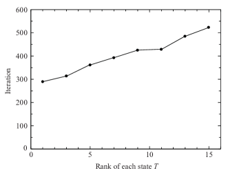
Figure 1: Example of numerical calculations for problem (57). The plots are the number of iterations to ensure that the difference between the upper and lower bounds for the optimal value is less than $10^{-9}$.

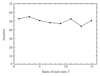
Figure 2: Example of numerical calculations for problem (60). The plots are the number of iterations to ensure that the difference between the upper and lower bounds for the optimal value is less than $10^{-9}$.

V Conclusion

We proposed an approach for finding an optimal quantum measurement for a generalized quantum state discrimination problem by using the modified version of the original problem. The modified problem is relatively easy to solve since it can be reduced to one of finding a minimum error measurement for a certain state set. We showed that the optimal values of the original problem can be derived from the Legendre transformation of the optimal values of the modified problem and that an optimal solution to the original problem can be obtained if an optimal solution to the corresponding modified problem can be computed. As an application of our approach, we presented an algorithm for numerically obtaining optimal solutions to generalized quantum state discrimination problems.

Appendix A Proof that $\hat{Y}^{(l)}$ in Eq. (37) is positive definite

We can prove this by induction as follows. First, let us consider the case of $l=0$. Let $\mathcal{Z}_{m}={\rm supp}~{}\hat{z}_{m}[\lambda^{(l)}]$. Note that $\mathcal{Z}_{m}$ is constant for any $\lambda^{(l)}$ with $\lambda_{j}^{(l)}>0$ $~{}(\forall j\in\mathcal{I}_{J})$. Since $\hat{D}_{m}^{(0)}=(\hat{z}_{m}[\lambda^{(0)}])^{2}/M$, i.e., ${\rm supp}~{}\hat{D}_{m}^{(0)}=\mathcal{Z}_{m}$, holds, we obtain

$${\rm supp}~{}\hat{Y}^{(0)} = \bigcup_{m=0}^{M-1}\mathcal{Z}_{m}=\mathcal{H},$$ (61)

which indicates that $\hat{Y}^{(0)}$ is positive definite. Next, assume that, for a certain $l>0$, ${\rm supp}~{}\hat{D}_{m}^{(l-1)}=\mathcal{Z}_{m}$ holds and $\hat{Y}^{(l-1)}$ is positive definite. From Algorithm 2, $\hat{D}_{m}^{(l)}$ can be expressed as

$$\hat{D}_{m}^{(l)} = \hat{z}_{m}[\lambda^{(l)}]\hat{\Lambda}^{(l-1)}\hat{D}_{m}^{(l-1)}\hat{\Lambda}^{(l-1)}\hat{z}_{m}[\lambda^{(l)}].$$ (62)

Since $\hat{\Lambda}^{(l-1)}=[\hat{Y}^{(l-1)}]^{-1/2}$ is positive definite and ${\rm supp}~{}\hat{D}_{m}^{(l-1)}=\mathcal{Z}_{m}$ holds, from Lemma 6 in Appendix B, ${\rm supp}~{}\hat{D}_{m}^{(l)}=\mathcal{Z}_{m}$. Therefore, similar to Eq. (61), $\hat{Y}^{(l)}$ is positive definite. $\blacksquare$

Appendix B Properties of support spaces

The aim of this section is to prove Lemma 6. As preparation, we make the following remark.

Remark 5

${\rm supp}~{}\hat{A}\hat{B}\hat{A}={\rm supp}~{}\hat{A}$ holds with positive semidefinite operators $\hat{A}$ and $\hat{B}$ satisfying ${\rm supp}~{}\hat{A}\subseteq{\rm supp}~{}\hat{B}$.

Proof

For any positive semidefinite operator $\hat{C}$, ${\rm supp}~{}\hat{C}$ can be expressed as

$${\rm supp}~{}\hat{C} = \{\ket{x}:\exists\alpha>0~{}{\rm such~{}that}~{}\hat{C}\geq\alpha\ket{x}\bra{x}\}.$$ (63)

For any positive real number $\varepsilon$ and $\ket{x}\in{\rm supp}~{}\hat{A}$, we have

$$\hat{A}\hat{B}\hat{A}-\varepsilon\ket{x}\bra{x} = \hat{A}(\hat{B}-\varepsilon\hat{A}^{+}\ket{x}\bra{x}\hat{A}^{+})\hat{A},$$ (64)

where $\hat{A}^{+}$ denotes the Moore-Penrose inverse operator of $\hat{A}$. Since $\hat{A}^{+}\ket{x}\in{\rm supp}~{}\hat{A}\subseteq{\rm supp}~{}\hat{B}$, if $\varepsilon$ is sufficiently small, then $\hat{B}\geq\varepsilon\hat{A}^{+}\ket{x}\bra{x}\hat{A}^{+}$ holds, which implies that the right-hand side of Eq. (64) is positive semidefinite. Thus, from Eq. (63), $\ket{x}\in{\rm supp}~{}\hat{A}\hat{B}\hat{A}$, i.e., ${\rm supp}~{}\hat{A}\hat{B}\hat{A}\supseteq{\rm supp}~{}\hat{A}$, holds. In contrast, we obtain

$$\dim({\rm supp}~{}\hat{A}\hat{B}\hat{A}) = {\rm rank}\hat{A}\hat{B}\hat{A}$$ (65)

$$\leq {\rm rank}\hat{A}=\dim({\rm supp}~{}\hat{A}).$$

Therefore, ${\rm supp}~{}\hat{A}\hat{B}\hat{A}={\rm supp}~{}\hat{A}$ holds. $\blacksquare$

Lemma 6

${\rm supp}~{}\hat{A}\hat{C}\hat{B}\hat{C}\hat{A}={\rm supp}~{}\hat{A}$ holds with positive semidefinite operators $\hat{A}$, $\hat{B}$, and $\hat{C}$ satisfying ${\rm supp}~{}\hat{A}\subseteq{\rm supp}~{}\hat{B}$ and ${\rm supp}~{}\hat{A}\subseteq{\rm supp}~{}\hat{C}$.

Proof

From ${\rm supp}~{}\hat{A}\subseteq{\rm supp}~{}\hat{B}$, there exists a positive real number $\delta$ such that $\hat{B}\geq\delta\hat{A}^{2}$. Indeed, we obtain

$$\hat{B} \geq \sigma_{B,\min}\hat{P}_{A}\geq\delta\hat{A}^{2}$$ (66)

with $\delta\leq\sigma_{B,\min}/\sigma_{A,\max}^{2}$, where $\hat{P}_{A}$, $\sigma_{B,\min}$, and $\sigma_{A,\max}$ are respectively the projection operator onto ${\rm supp}~{}\hat{A}$, the minimum positive eigenvalue of $\hat{B}$, and the maximum eigenvalue of $\hat{A}$. Thus, we obtain

$$\hat{A}\hat{C}\hat{B}\hat{C}\hat{A} \geq \delta\hat{A}\hat{C}\hat{A}^{2}\hat{C}\hat{A}=\delta(\hat{A}\hat{C}\hat{A})^{2},$$ (67)

which yields ${\rm supp}~{}\hat{A}\hat{C}\hat{B}\hat{C}\hat{A}\supseteq{\rm supp}~{}\hat{A}\hat{C}\hat{A}$. In contrast, ${\rm supp}~{}\hat{A}\hat{C}\hat{A}={\rm supp}~{}\hat{A}$ holds from Remark 5. Therefore, ${\rm supp}~{}\hat{A}\hat{C}\hat{B}\hat{C}\hat{A}\supseteq{\rm supp}~{}\hat{A}$ holds. Moreover, similar to Eq. (65), we have $\dim({\rm supp}~{}\hat{A}\hat{C}\hat{B}\hat{C}\hat{A})\leq\dim({\rm supp}~{}\hat{A})$, and thus ${\rm supp}~{}\hat{A}\hat{C}\hat{B}\hat{C}\hat{A}={\rm supp}~{}\hat{A}$ holds. $\blacksquare$

Appendix C Monotonically increasing property of $\beta_{j}$ with respect to $\lambda$

Lemma 7

Let $\lambda,\lambda^{\prime}\in\mathbf{R}_{+}^{J}$ satisfy $\lambda_{k}<\lambda_{k}^{\prime}$ and $\lambda_{j}=\lambda_{j}^{\prime}$ $~{}(\mathcal{I}_{J}\ni j\neq k)$ for a certain $k\in\mathcal{I}_{J}$. Also, let $\Pi$ and $\Pi^{\prime}$ be optimal solutions for problem P2 with respect to $\lambda$ and $\lambda^{\prime}$, respectively. Then, $\beta_{k}(\Pi)\leq\beta_{k}(\Pi^{\prime})$ holds.

Proof

Suppose for contradiction that $\beta_{k}(\Pi)>\beta_{k}(\Pi^{\prime})$. From the definition of $\hat{z}_{m}(\lambda)$ in Eq. (18), we have that for any POVM $\Phi\in\mathcal{M}_{M}$,

$$g(\Phi;\lambda^{\prime}) = \sum_{m=0}^{M-1}{\rm Tr}[\hat{z}_{m}(\lambda^{\prime})\hat{\Phi}_{m}]$$ (68)

$$= \sum_{m=0}^{M-1}{\rm Tr}\left[[\hat{z}_{m}(\lambda)+(\lambda^{\prime}_{k}-\lambda_{k})\hat{a}_{k,m}]\hat{\Phi}_{m}\right]$$

$$= g(\Phi;\lambda)+(\lambda^{\prime}_{k}-\lambda_{k})\beta_{k}(\Phi).$$

Thus, we obtain

$$g(\Pi^{\prime};\lambda^{\prime}) = g(\Pi^{\prime};\lambda)+(\lambda^{\prime}_{k}-\lambda_{k})\beta_{k}(\Pi^{\prime})$$ (69)

$$\leq g(\Pi;\lambda)+(\lambda^{\prime}_{k}-\lambda_{k})\beta_{k}(\Pi^{\prime})$$

$$< g(\Pi;\lambda)+(\lambda^{\prime}_{k}-\lambda_{k})\beta_{k}(\Pi)$$

$$= g(\Pi;\lambda^{\prime}),$$

where the first and fourth lines follow from Eq. (68). The second line follows from $\Pi$ being an optimal solution to problem P2 with respect to $\lambda$. Equation (69) contradicts the assumption that $\Pi^{\prime}$ is an optimal solution to problem P2 with respect to $\lambda^{\prime}$. $\blacksquare$

References

- Holevo (1973) A. S. Holevo, J. Multivar. Anal. 3, 337 (1973).
- Helstrom (1976) C. W. Helstrom, Quantum detection and estimation theory (Academic Press, 1976).
- Yuen et al. (1975) H. P. Yuen, K. S. Kennedy, and M. Lax, IEEE Trans. Inf. Theory 21, 125 (1975).
- Eldar et al. (2003) Y. C. Eldar, A. Megretski, and G. C. Verghese, IEEE Trans. Inf. Theory 49, 1007 (2003).
- Belavkin (1975) V. P. Belavkin, Stochastics 1, 315 (1975).
- Ban et al. (1997) M. Ban, K. Kurokawa, R. Momose, and O. Hirota, Int. J. Theor. Phys. 36, 1269 (1997).
- Usuda et al. (1999) T. S. Usuda, I. Takumi, M. Hata, and O. Hirota, Phys. Lett. A 256, 104 (1999).
- Eldar and Forney Jr. (2001) Y. C. Eldar and G. D. Forney Jr., IEEE Trans. Inf. Theory 47, 858 (2001).
- Ivanovic (1987) I. D. Ivanovic, Phys. Lett. A 123, 257 (1987).
- Dieks (1988) D. Dieks, Phys. Lett. A 126, 303 (1988).
- Peres (1988) A. Peres, Phys. Lett. A 128, 19 (1988).
- Eldar (2003a) Y. C. Eldar, IEEE Trans. Inf. Theory 49, 446 (2003a).
- Herzog (2007) U. Herzog, Phys. Rev. A 75, 052309 (2007).
- Pang and Wu (2009) S. Pang and S. Wu, Phys. Rev. A 80, 052320 (2009).
- Kleinmann et al. (2010) M. Kleinmann, H. Kampermann, and D. Bruß, J. Math. Phys. 51, 032201 (2010).
- Roa et al. (2011) L. Roa, C. Hermann-Avigliano, R. Salazar, and A. Klimov, Phys. Rev. A 84, 014302 (2011).
- Bergou et al. (2012) J. A. Bergou, U. Futschik, and E. Feldman, Phys. Rev. Lett. 108, 250502 (2012).
- Bandyopadhyay (2014) S. Bandyopadhyay, Phys. Rev. A 90, 030301(R) (2014).
- Chefles and Barnett (1998) A. Chefles and S. M. Barnett, J. Mod. Opt. 45, 1295 (1998).
- Eldar (2003b) Y. C. Eldar, Phys. Rev. A 67, 042309 (2003b).
- Fiurášek and Ježek (2003) J. Fiurášek and M. Ježek, Phys. Rev. A 67, 012321 (2003).
- Herzog (2012) U. Herzog, Phys. Rev. A 86, 032314 (2012).
- Nakahira et al. (2012) K. Nakahira, T. S. Usuda, and K. Kato, Phys. Rev. A 86, 032316 (2012).
- Bagan et al. (2012) E. Bagan, R. Muñoz-Tapia, G. A. Olivares-Renteria, and J. A. Bergou, Phys. Rev. A 86, 040303 (2012).
- Herzog (2015) U. Herzog, Phys. Rev. A 91, 042338 (2015).
- Touzel et al. (2007) M. A. P. Touzel, R. B. A. Adamson, and A. M. Steinberg, Phys. Rev. A 76, 062314 (2007).
- Hayashi et al. (2008) A. Hayashi, T. Hashimoto, and M. Horibe, Phys. Rev. A 78, 012333 (2008).
- Sugimoto et al. (2009) H. Sugimoto, T. Hashimoto, M. Horibe, and A. Hayashi, Phys. Rev. A 80, 052322 (2009).
- Holevo (1982) A. S. Holevo, Probabilistic and statistical aspects of quantum theory, Vol. 1 (North-Holland, Amsterdam, 1982).
- Paris (1997) M. G. Paris, Phys. Lett. A 225, 23 (1997).
- Nakahira et al. (2015a) K. Nakahira, K. Kato, and T. S. Usuda, Phys. Rev. A 91, 052304 (2015a).
- Nakahira et al. (2015b) K. Nakahira, K. Kato, and T. S. Usuda, Phys. Rev. A 91, 022331 (2015b).
- Hiriart-Urruty and Lemaréchal (2001) J.-B. Hiriart-Urruty and C. Lemaréchal, Fundamentals of convex analysis (Springer Verlag, New York, 2001).
- Usuda et al. (2002) T. S. Usuda, S. Usami, I. Takumi, and M. Hata, Phys. Lett. A 305, 125 (2002).
- Andersson et al. (2002) E. Andersson, S. M. Barnett, C. R. Gilson, and K. Hunter, Phys. Rev. A 65, 052308 (2002).
- Eldar et al. (2004) Y. C. Eldar, A. Megretski, and G. C. Verghese, IEEE Trans. Inf. Theory 50, 1198 (2004).
- Herzog (2004) U. Herzog, J. Opt. B: Quantum Semiclass. Opt. 6, S24 (2004).
- Deconinck and Terhal (2010) M. E. Deconinck and B. M. Terhal, Phys. Rev. A 81, 062304 (2010).
- Zibulevsky and Elad (2010) M. Zibulevsky and M. Elad, Signal Processing Magazine, IEEE 27, 76 (2010).
- Ježek et al. (2002) M. Ježek, J. Řeháček, and J. Fiurášek, Phys. Rev. A 65, 060301 (2002).
- Horn and Johnson (1985) R. A. Horn and C. R. Johnson, Matrix analysis (Cambridge university press, New York, 1985).
- Reimpell and Werner (2005) M. Reimpell and R. Werner, Phys. Rev. Lett. 94, 080501 (2005).
- Reimpell (2007) M. Reimpell, Matrix analysis (Ph.D. thesis, Technische Universität, 2007).
- Tyson (2010) J. Tyson, J. Math. Phys. 51, 092204 (2010).
- Nakahira et al. (2015c) K. Nakahira, K. Kato, and T. S. Usuda, Phys. Rev. A 91, 012318 (2015c).
- Borchers (1999) B. Borchers, Optimization Methods and Software 11, 613 (1999).