Periodic transit and variability search with simultaneous systematics filtering: Is it worth it?

By using subsets of the HATNet and K2 (Kepler two-wheel) Campaign 1 databases, we examine the effectiveness of filtering out systematics from photometric time series while simultaneously searching for periodic signals. We carry out tests to recover simulated sinusoidal and transit signals added to time series with both real and artificial noise. We find that the simple (and more traditional) method that performs correction for systematics first and signal search thereafter, produces higher signal recovery rates on the average, while also being substantially faster than the simultaneous method. Independently of the method of search, once the signal is found, a far less time consuming full-fledged model, incorporating both the signal and systematics, must be employed to recover the correct signal shape. As a by-product of the tests on the K2 data, we find that for longer period sinusoidal signals the detection rate decreases (after an optimum value is reached) as the number of light curves used for systematics filtering increases. The decline of the detection rate is observable in both methods of filtering, albeit the simultaneous method performs better in the regime of relative high template number. We suspect that the observed phenomenon is linked to the increased role of low amplitude intrinsic stellar variability in the space-based data. This assumption is also supported by the substantially higher stability of the detection rates for transit signals against the increase of the template number.

1 Introduction

The filtering of instrumental and environmental effects from astronomical time series data is a vital ingredient in the data processing pipelines for the time series collected by transiting extrasolar planet (TEP) search projects. The reason why systematics filtering is so important in the search for TEPs is that these surveys ‘indiscriminately’ examine basically all stars (except perhaps obvious giants) available in their photometric databases. Therefore, small systematics of the size of few percent or less become significant due to the leakage of their power (directly or via their harmonics) to the frequency range of interest and thereby blur the signal. Except for the aliasing, space-based surveys (CoRoT and Kepler) suffer from the same problem.

Although there is a weak resemblance between today’s systematics filtering methods and the widely used simple ensemble photometry (e.g., Honeycutt honeycutt1992 (1992)), there is also a basic difference. In the case of ensemble photometry we do not fit the target light curve (LC) by time series carrying information on the systematics but rather assume that all stars in the field are affected by the same transparency change that can be accurately estimated by averaging out all incoming fluxes from the individual stars. With the division of the target flux by the ensemble flux, we filter out systematic variations that are common to all stars, but any differences between sources (due to e.g. local topology, subpixel structure, etc.) are not corrected for.

Modern methods of systematics filtering assume that the systematics are specific to each star, but they can be built up as the linear combinations of the systematics of other stars (or with the aid of other auxiliary measurable quantities, e.g., the width of the point spread function). The determination of the optimum linear combination is usually performed by standard least squares technique.

This approach is drastically different from the one followed by the ensemble method, because here the LCs are ‘flattened out’ as much as possible, which may lead to a substantial depression of the signal we are searching for. The success of the method depends on the relative degree of depression of the systematics and the signal. It is expected that in general, the signal ‘wins’, since its properties are usually less common with those of the other LCs, whereas the contributing systematic effects are more likely shared also with other stars in the field.

The method was implemented first in the Trend Filtering Algorithm (TFA, Kovács, Bakos, & Noyes kovacs2005 (2005)) and in SysRem (Tamuz, Mazeh, & Zucker tamuz2005 (2005)). While TFA uses a ‘brute force’ fit of many (several hundred) nearly randomly selected template stars from the target field, SysRem employs an iterative algorithm that results in a lower final number of correcting time series (albeit this number may not be well-defined in practice). This correcting set is built up from a large number of LCs of the target field, similarly to the popular Principal Component Analysis (PCA). Both of these methods can be run in ‘reconstructive’ mode, with full (systematics$+$signal) model fit, once the signal frequency is found (and, in the case of SysRem, once the basis of trends has been determined). This results in a much better reproduction of the original signal shape and cures the depression caused in the signal search phase.

In spite of the ability of reconstructing the signal after its initial detection, efforts have been made to decrease the level of signal depression and minimize the chance of possible signal loss during the signal search phase of the analysis. This has usually been tackled by a careful selection of the template time series, keeping their number to a minimum and introducing more general probabilistic (i.e., Bayesian) treatment of the problem. Kim et al. (kim2009 (2009)) use a hierarchical clustering method to select an optimum number of co-trending LCs. Chang, Byun, & Hartman (chang2015 (2015)) adopt the same method as part of their pipeline for precise cluster photometry. A PCA-based criterion is used in the algorithm proposed by Petigura & Marcy (petigura2012 (2012)) for the analysis of the Kepler LCs. The more involved, PDC-MAP pipeline (Stumpe et al. smith2012 (2012); Smith et al. smith2012 (2012)) of the Kepler mission also utilizes PCA for selecting the basis vectors for the systematics correction. In a similar manner, Roberts et al. (roberts2013 (2013)) discuss the advantage of using Bayesian linear regression for robust filtering and employ entropy criterion for selecting the most relevant corrections while maintaining the original signal as much as possible.

The method has also been extended by including additional effects, such as stellar variability (Alapini & Aigrain alapini2009 (2009), Kovács & Bakos kovacs2008 (2008)) and simultaneously considering multiplicative and additive systematics, both of which may be relevant when a wide brightness range is considered (e.g., in the CoRoT data, see the SARS algorithm by Ofir et al. ofir2010 (2010)).

The K2 mission (the successful continuation of the Kepler mission using two reaction wheels – see Howell et al. howell2014 (2014)) inspired further ideas to revisit the problem of trend filtering. Several papers have been published on this subject, focusing mainly on the wobble of the spacecraft due to the periodic ignition of the thrusters, to stabilize the pointing. Vanderburg & Johnson (vanderburg2014 (2014)) employed a simple, yet effective method to correct for effects due to the wobble. Their method utilizes the non-linear correlation between the pixel position and flux variation, and leads to a substantial (a factor of $2-5$) improvement in the RMS of the light curves. The method of Vanderburg & Johnson (vanderburg2014 (2014)) is a specific extension of the method of light curve correction based on image properties (external parameter decorrelation, EPD, see Bakos et al. bakos2010 (2010) for ground-based wide-field surveys, and those of, e.g., Knutson et al. knutson2008 (2008) and Cubillos et al. cubillos2014 (2014) for the treatment of the Spitzer planet transit and occultation data). In a very recent paper by Huang et al. (huang2015 (2015)) the authors employ a combination of various filtering techniques (including EPD, TFA and Fourier) and, in the most favorable brightness range, reach a precision of $15$–$20$ ppm on a $6.5$ hours time span – i.e., hitting the precision of the original Kepler mission.

Focusing also on the roll angle variation in the K2 data, Aigrain et al. (aigrain2015 (2015)) developed a method based on the simultaneous modeling of this particular systematics and intrinsic stellar variability within the framework of Gaussian processes. This allows for a great flexibility in determining the target-dependent effect of the roll angle variation, together with the conservation of the intrinsic signal. The authors report broad agreement in the gain of precision with the one obtained by Vanderburg & Johnson (vanderburg2014 (2014)).

Foreman-Mackey et al. (foreman2015 (2015)) do not focus on the roll angle variation alone but use a relative large number of eigen LCs from their PCA to model the K2 LCs as the linear combination of these eigen LCs and a transit model. Similarly to the approach of Aigrain et al. (aigrain2015 (2015)), this is also a full time series modeling in the sense that they conduct a simultaneous search for the best-fitting combination of systematics and signals. For the computationally challenging task of searching for the transit parameters while finding also the true contribution of the systematics, Foreman-Mackey et al. (foreman2015 (2015)) opt for the maximum likelihood approach in which it is assumed that the transit events are independent. With this assumption the joint distribution function can be computed as a product of the likelihoods of the individual events. This observation allows a considerable speed up of the otherwise slow minimization process, since a part of the computation can be performed on a coarse parameter grid that can be used thereafter for the fine grid search by simply interpolating on the coarse grid. Although the authors do not deal with the precision of their finally derived LCs, from their Figure 2 and Table 1 of Vanderburg & Johnson (vanderburg2014 (2014)) it seems that they both reach similar precision of $\sim 33$ ppm on an integration time span of $6$ hours. This is only $50$ % larger than the corresponding figure for the original Kepler mission in the same brightness range of $11-12$ mag. In a subsequent paper the method is extended to general variability search by using a Fourier, instead of a boxcar representation of the signal (Angus et al. angus2015 (2015)).

Yet another recent work by Wang et al. (wang2015 (2015)) introduces a different method aiming at simultaneous systematics filtering and signal preservation. The method (Causal Pixel Model) is based on the autoregressive and co-trended maximum likelihood estimate of each pixel flux associated with a given target. Each time series value is predicted from a fit computed by the omission of the values close in time to that observation. The size of the window of omission is chosen freely based on the expected duration of the transit event. By construction, the resulting filter is transit signal preserving (but, because of the autoregressive fit, it is also a stellar variability ‘killer’). The authors report a consistently better performance of their method when compared to the standard Kepler pipeline PDC.

The idea of the full-fledged (i.e., systematics$+$signal) search has also come up in the context of ground-based surveys. To increase of the transit detection capability of the MEarth project, Berta et al. (berta2012 (2012)) employ a nightly full model fit to the target LCs and then combine the individual likelihood functions into a joint likelihood. The solution found with this probabilistic approach helps to avoid nightly overfitting, which is a common problem in multi-parametric fits of small datasets.

Stimulated by the above efforts, this paper deals with the performance of the full-fledged frequency search. Naturally, the full model approach is preferable once the signal period is found (Kovács et al. kovacs2005 (2005)). Also, by fitting systematics only, the underlying signal suffers from some level of depression, which jeopardizes the detection capability. However, it is unclear if in the period search phase the increased degree of freedom due to the inclusion of the signal model in the systematics fit will not increase the false alarm rate. Last but not least, for signal search, the full model approach is much more intensive computationally than the partial model fit (i.e., assuming no signal, fitting only the systematics and performing the signal search on the residuals thereafter). Therefore, it is important to investigate if the full model search is worth the effort (i.e., if the increased complexity and execution time is compensated by the increased detection efficiency).

2 Simultaneous fit for systematics and periodic signal

Let us assume that the photometric pipeline supplies a large set of time series $\{x(j,i);j=1,2,...,L;i=1,2,...,N\}$, containing $L$ light curves, each with $N$ data points, and, for simplicity, sampled on the same timebase $\{t(i);i=1,2,...,N\}$. Following the TFA methodology (for simplicity) we model each of the observed time series as a linear combination of suitably chosen $M$ cotrending light curves and a Fourier sum of arbitrary order $K/2$. For any target time series $\{y(i);i=1,2,...,N\}$ (selected from $\{x(j,i)\}$) at any given trial frequency $\nu$ we minimize the residuals ${\cal D}$ between the model and data following the standard least squares (LS) approach

$${\cal D}=\sum_{i=1}^{N}\left(y(i)-\sum_{j=1}^{M}a_{\rm j}S(j,i)-\sum_{j=1}^{K+1}b_{\rm j}F(j,i)\right)^{2}\hskip 5.69054pt,$$ (1)

where $\{S(j,i);j=1,2,...,M;i=1,2,...,N\}$ denote the set of cotrending time series and $\{F(j,i);j=1,2,...,K+1;i=1,2,...,N\}$ stand for the Fourier representation of the underlying signal. In particular, at any given instant of time $t(i)$, $F(1,i)=1,F(2,i)=\sin(\varphi),F(3,i)=\cos(\varphi),...,F(K,i)=\sin(K\varphi),F(K+1,i)=\cos(K\varphi)$, with phase $\varphi=2\pi\,\nu\,t(i)$ (and, of course, the reference epoch for $\{t(i)\}$ is arbitrary).

The LS condition above leads to normal matrix schematically shown in Fig. 1. We see that when scanning the various test frequencies, the TFA part of the matrix (typically the dominant part of the full matrix) does not change. This block structure of the normal matrix allows us to ease the otherwise very heavy computational load required by the re-computation and inversion of the normal matrix each time a new frequency is tested.

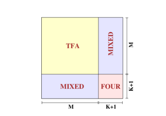
Figure 1: Main blocks of the normal matrix of the full-fledged systematics filtering least squares problem (see Eqs. (1), (2)). In the course of the period search, only the MIXED and FOUR blocks change (the latter containing the pure Fourier terms of the fit).

In detail, the following set of linear equations is obtained when satisfying the LS condition posed by Eq. (1)

$$\left(\begin{array}[]{lr}TF&MI^{T}\\ MI&FO\end{array}\right)\hskip 0.0pt\left(\begin{array}[]{cc}a\\ b\end{array}\right)\hskip 0.0pt=\left(\begin{array}[]{cc}YT\\ YF\end{array}\right)\hskip 5.69054pt,$$ (2)

where $\{a\}$ and $\{b\}$ are, respectively, $M$- and $K+1$-dimensional column vectors. The block elements of the normal matrix and the right-hand-side vectors are computed as follows:

$$TF(i,j) = \sum_{k=1}^{N}S(i,k)S(j,k)\hskip 2.84526pt,1\leq i\leq M,1\leq j\leq M$$

$$MI(i,j) = \sum_{k=1}^{N}F(i,k)S(j,k)\hskip 2.84526pt,1\leq i\leq K+1,1\leq j\leq M$$

$$MI^{T}(i,j) = \sum_{k=1}^{N}S(i,k)F(j,k)\hskip 2.84526pt,1\leq i\leq M,1\leq j\leq K+1$$

$$FO(i,j) = \sum_{k=1}^{N}F(i,k)F(j,k)\hskip 2.84526pt,1\leq i\leq K+1,1\leq j\leq K+1$$

$$YT(i) = \sum_{k=1}^{N}S(i,k)y(k)\hskip 2.84526pt,1\leq i\leq M$$

$$YF(i) = \sum_{k=1}^{N}F(i,k)y(k)\hskip 2.84526pt,1\leq i\leq K+1\hskip 5.69054pt.$$ (3)

In solving Eq. (2) first we observe that the cotrending (TFA) part needs to be computed only once, since this is constant during the frequency scan. Furthermore, if we opt for solving the system with matrix inversion, we can utilize the formula valid for block matrix inversion, that may also give some advantage in decreasing the computational load. Further speed-up can be gained by utilizing the positive definitive nature of the normal matrix and use, e.g., Cholesky factorization, or the more general QR decomposition (e.g., Press et al. press1992 (1992)). The inverse of the normal matrix of Eq. (2) constitutes the following blocks (the Helmert-Wolf blocking, see the proof by Banachiewicz banachiewicz1937 (1937) and applications, e.g., by Rajan & Mathew rajan2012 (2012)):

$$\left(\begin{array}[]{lr}TF&MI^{T}\\ MI&FO\end{array}\right)^{-1}=\left(\begin{array}[]{lr}TF^{-1}+G*MI*TF^{-1}&-G\\ -SC^{-1}*MI*TF^{-1}&SC^{-1}\end{array}\right)\hskip 5.69054pt.$$ (8)

In the above eqations symbol $*$ denotes matrix multiplication, $SC$ is the Schur complement of the normal matrix ($SC=FO-MI*TF^{-1}*MI^{T}$) and $G=TF^{-1}*MI^{T}*SC^{-1}$. Although employing these formulae for the inversion results in an increase of $20$–$30$% in the speed of execution (relative to the simple Gaussian inversion of the full matrix), the full-fledged systematics filtering is still very expensive, due to the large size of matrix $TF$, carrying the information on systematics. Our experience shows that for a moderate size time series (e.g., with few thousand data points) and $200$ TFA template time series the full-fledged (hereafter tfadft) search is $2$–$3$-times slower than the “filter first, search for signals thereafter”-method (hereafter tfa+dft). With doubling the TFA template size this ratio increases to nearly $10$.

Within the above framework we can substitute the model functions $\{F(j,i)\}$ with any other, frequency-dependent functions, better representing the signal to be searched for. We can also allow for additional non-linear parameters in the model functions, further increasing the complexity of the problem (see Foreman-Mackey et. al foreman2015 (2015) for boxcar signals). Although Fourier representation is sub-optimal for transit signals (Kovács, Zucker, & Mazeh kovacs2002 (2002)), for the purpose of this paper it is suitable, since both the tfadft and the tfa+dft models are tested within the same framework. Additional applications of the Fourier base for transit search can be found in Moutou et al. (moutou2005 (2005)) and Samsing (samsing2015 (2015)).

3 Comparison of the performances of the time series models

Here we report on a detailed numerical testing of the full time series model fit (tfadft) and the two-step partial fit (tfa+dft). Our testing ground is the frequency spectra of the various test signals. These frequency spectra are based on the RMS of the residuals of the fitted data (see Eq. (1)). To retain the more traditional pattern of the frequency spectra, the residual spectra are obtained from D as follows

$$P(\nu)={\sqrt{\cal D}-\sqrt{\cal D_{\rm max}}\over\sqrt{\cal D_{\rm min}}-\sqrt{\cal D_{\rm max}}}\hskip 5.69054pt,$$ (9)

where the indices refer to the max/min values of D. The function $P(\nu)$ is akin to the amplitude spectrum and it is obviously confined to $[0,1]$. The characterization of the signal-to-noise ratio of the highest peak in $P(\nu)$ goes in the standard way

$${\rm SNR}={P(\nu_{0})-{<}\,P(\nu)\,{>}\over\sigma(P(\nu))}\hskip 5.69054pt.$$ (10)

Here $P(\nu_{0})$, ${<}\,P(\nu)\,{>}$ and $\sigma(P(\nu))$ denote, respectively, the power at the peak frequency, the average of the power over the waveband where the SNR is referred to and the standard deviation of the ‘grass’ (i.e., the noise) component of the spectrum. This latter phrase means that we omit ‘outliers’ (i.e., high peaks) when $\sigma(P(\nu))$ is computed. Please note that with the above definition SNR can be a sensitive function of the waveband of reference, especially if the noise is colored.

In the following we perform a two-step analysis of the efficiency of the tfadft and tfa+dft approaches to systematics filtering. In the first step we examine the signal recovery properties of these methods on a simple two-component time series. Then, using subsets of the databases of the HATNet and K2 projects, we inject various signals in the observed data and check the discovery rates for the two methods.

3.1 Two-component signal test

We start with the simplest possible scenario of two noisy sine functions with known parameters.

$$y(i) = g(i)+A_{2}\sin(2\pi\nu_{2}t_{\rm i})+gn2(i)$$

$$g(i) = A_{1}\sin(2\pi\nu_{1}t_{\rm i})+gn1(i)\hskip 5.69054pt.$$ (11)

Here $gn1$ and $gn2$ denote independent Gaussian white noise. Function $g$ is considered as being the contribution from the systematics, whereas the second sine component constitutes the signal we are searching for. In this basic test we make function $g$ known for the routines. Under this circumstance, tfadft should yield an exact match to the data, if the signal is noiseless ($gn2=0$). Therefore, the more interesting question is what happens if we increase the noise component of the signal. We examine this question for $100$ signal frequencies by uniformly scanning the $[0.4,0.5]$d^-1 frequency range. Other time series parameters are fixed to the following values: $A_{1}=0.02$, $\nu_{1}=0.45$, $\sigma_{1}=0.001$, $A_{2}=0.01$ and $\sigma_{2}=0.06$ for the low- and $\sigma_{2}=0.0001$ for the high-SNR case. For each signal frequency we add the same realization of the noise to the signal to keep track only of the effect of changing signal frequency. For sensing the effect of noise realization, we repeat the frequency scan for $10$ different realizations. All tests are performed on the timebase of one of the light curves from the HATNet field to be described in Sect. 3.2.

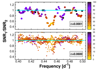
Figure 2: Variation of the SNR ratios of the tfa+dft (SNR₁) and tfadft (SNR₂) spectra as a function of the injected signal frequency for the two-component time series described in the text. The shading is proportional to SNR₂ as indicated by the sidebars. For realistic (noisy) time series, the signal detection capability of the two methods become nearly the same. The result shown in the bottom panel is based on $10$ realizations of the Gaussian noise added to the time series.

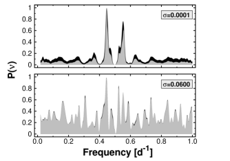
Figure 3: Illustration of the dependence of the frequency spectra on noise level (upper vs lower panels) and on the method of data analysis (lighter shade: full time series model; darker shade: partial time series model). In this example the frequency of the test signal is $0.446$d^-1, very close to that of the systematics. Farther away from the frequency of the systematics the difference between the two methods is much smaller, even in the noiseless case.

The dependence of the SNR of the frequency spectra on the signal frequency with the above fixed component of systematics is shown in Fig. 2. As expected, the high-SNR case (upper panel) clearly shows the advantage of the full model fit over the partial one in the immediate neighborhood of the frequency of the systematics. However, it is important to note that in this high-SNR range the better performance of tfadft does not have much use, since in both cases the signal is detected with very high significance, even in the close neighborhood of the frequency of the systematics. For low SNR the situation changes, and the difference between the two models diminishes, as shown in the bottom panel of Fig. 2. Although there is still some signal frequency dependence (affected by noise realization), most of the SNR values are equal within $\sim 10$%, with a slight preference toward the partial model.

For a more straightforward illustration of the convergence of the two signal search methods as the noise is increased, in Fig. 3 we display the frequency spectra related to the test with the signal frequency $0.446$d^-1 (very close to $0.45$d^-1, the frequency of the systematics, which is the regime where tfadft is expected to provide the greatest performance enhancement over tfa+dft). From the figure it is clear that tfadft outperforms tfa+dft when the noise level is very low (when, however, the detection is not a problem for either of the methods). On the other hand, at a more reasonable noise level the two methods behave comparably.

We conclude from this simple test (clearly favorable for the full time series model) that, in general, from pure signal detection point of view, the full model does not necessarily have advantage over the partial one that may justify its use. In specific cases of nearly coinciding signal and systematics frequencies we may gain some advantage from the full model, but it is unclear if the slightly larger detection power is worth the additional computational burden (especially in more realistic cases with high TFA template numbers - see Sect. 3.3).

3.2 Ensemble test: datasets and signals

In the previous section we used test data that were purely artificial, with known systematics and signal. However, for real observations we do not know the exact form of the systematics. In this case we build up (if possible) a simple model for the systematics and use this as an approximation of the true systematics. In practice, however inexact this approach is, it usually leads to very impressive improvement in signal detection rates. In the present context the inexact model for the systematics acts as an unknown noise component, influencing also the ‘full’ time series models and making them more similar to the partial models. Whether this ‘less partial’ model is able to outperform the ‘fully partial’ model (based on separate systematics and signal fits) depends on the fraction of the unknown constituents in the adopted model of systematics and other factors, e.g., the spectral behavior of the time series at frequencies different from that of the signal.

We inject various signals into sub-samples of light curves observed by HATNet (Bakos et al. bakos2004 (2004)) and by the Kepler two-wheel mission during the phase of Campaign 1 (K2, Howell et al. howell2014 (2014)). The light curves from the HATNet database have properties that are typical for HATNet observations: they have been collected from a $10^{\circ}\times 10^{\circ}$ field, containing nearly $39000$ objects from $\sim 6$ mag to $\sim 14$ mag (in Sloan r-band). Each object has a photometric time series with up to $8600$ datapoints spanning $165$ days. For economical testing we choose only the first $2000$ data points from each time series – this cut decreases the time span down to $51$ days. We limit our study to $300$ objects at the brighter magnitude end between $8.4$ and $9.1$ mag. Most of these objects suffer from saturated pixels, due to their bright magnitudes (see Fig. 4). Because of their large systematics, we select these objects to sense the differences between the methods tested more effectively. We choose the EPD (External Parameter Deconvolved) LCs – see Bakos et. al. (bakos2010 (2010)). Although these LCs are largely free from strong systematics, TFA introduces further improvements.

For a quick and easy access to the light curves of Campaign 1 of the K2 mission, we resort to the depository of the K2 HAT Light Curve project as described by Huang et al. (huang2015 (2015)). To remain statistically compatible with the sample size used in the test of the HATNet data, we select a sample of $300$ stars from their object-summary.csv file. All these stars have UCAC4 identifications with Johnson $V$ magnitudes, which we use to constrain the sample between $V=9.59$–$10.44$ mag. Unlike Huang et al. (huang2015 (2015)), we include objects from all channels, both in the sample of these $300$ stars and also in the selected TFA templates (this enables us to use larger template numbers). For the templates we restrict the selection to stars brighter than $V=11.5$ mag. As for the HATNet data, we constrain the original number of data points per LC of $3820$ to $2000$. This cut decreses the time span of the data from $82$ days to $44$ days. At all template numbers the templates are distributed on a nearly uniform grid in the full field of view (following the original idea of template selection as described in Kovács et al. kovacs2005 (2005)). We use the best aperture light curves and select the direct photometric values (column #5 in the light curve files, annotated as IM##, where ## denotes the aperture size). Although using these direct photometric values have the advantage of performing our injected signal tests as ‘purely’ as possible, it is sub-optimal in terms of the accessible signal sensitivity, since it lacks EPD correction, which carries away a great part of the systematics in the K2 data. We note that for the HATNet data our choice of the EPD magnitudes is justified on the basis of the large variation of the original photometric fluxes, which makes outlier handling more cumbersome in the TFA analysis (in the case of the K2 data the straight photometric fluxes behave in a way that is more easy to tackle).

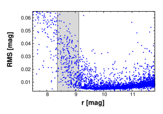
Figure 4: Magnitude-RMS plot for HATNet field #317 (TFA-filtered data with high TFA template number of $990$ are plotted). Shaded area shows the region of the $300$ stars we choose for the tests presented in this paper.

Two basic signal types are tested. The first one is a simple sinusoidal signal whereas the second one is a periodic transit signal. As shown in Table 1, the combination of the periods, amplitudes (transit depths) are different for the seven test signals. In all cases the amplitudes are selected to be low enough to avoid detection in the non-filtered (original) data but high enough to allow detection in the systematics-filtered data. Periods are chosen to be short enough to avoid data sampling issues in the case of the the transit signal when testing the HATNet data. Signals #1 and #2 are used for testing the HATNet data, whereas #3 – #7 are employed on the K2 data. For the latter, #3 and #4 are akin to #1 and #2, except for their amplitudes, that are adjusted to the considerable lower noise level of the K2 data. Signal #5 is intended to demonstrate the stabilization of the detection rate for sinusoidal signals in the K2 data by the decrease of the period. The longer period sinusoidal signal #6 (along with the somewhat shorter period signal #3) is for showing the impaired detection rate for longer period sinusoidal signals on the K2 data at higher TFA template numbers. Signal #7 is devoted to show the opposite behavior of the transit signals on the same dataset even at these longer periods.

As mentioned, we opted for using a Fourier-based representation of the signals to be tested, in spite of the poor capability of the Fourier decomposition in the case of more appropriate (i.e., short event duration) transit signals. Furthermore, within the framework of standard LS fitting, with the increasing order of the Fourier sum, it becomes more vulnerable against data gaps and outlying data points. Therefore, by choosing a long transit length (relative to the period), more representative for short period systems, we are able to use a reasonably low-order Fourier sum that is stable but still yields an acceptable representation of the transit shape (see Fig. 5).

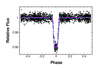
Figure 5: Illustration of the Fourier approximation of the transit-like signal #2. The synthetic trapezoidal signal is shown by pink line. Black dots show the synthetic signal after adding a Gaussian noise with $\sigma=0.003$. The result of a 10-th order Fourier fit to these noisy data is shown by light blue line.

Table 1: Test signal parameters

Name	Type	Ampl.	Freq.	$Q_{\rm tran}$
$\#1$	sine	$0.0100$	$0.24$	$-$
$\#2$	transit	$0.0400$	$0.64$	$0.10$
$\#3$	sine	$0.0002$	$0.24$	$-$
$\#4$	transit	$0.0005$	$0.64$	$0.10$
$\#5$	sine	$0.0001$	$0.64$	$-$
$\#6$	sine	$0.0001$	$0.21$	$-$
$\#7$	transit	$0.0005$	$0.21$	$0.10$

Notes: Amplitudes/transit depths and frequencies are given in relative fluxes and [$d^{-1}$], respectively. The ratio of the total transit time to the period is denoted by $Q_{\rm tran}$. The phase of the transit is chosen to yield near the average expected number (i.e., Q${}_{\rm tran}\times N=200$) of in-transit data points for the HATNet data. Signals #3 – #7 are used for testing the K2 data (see Sect. 3.4).

3.3 Ensemble test: results based on HATNet

By injecting known test signals in the target light curves we are able to check if the signal is detectable in the LS Fourier spectra. Instead of giving only a lower SNR limit as the sole detection criterion, which must be employed for unknown signals, here we utilize the fact that the signal frequency is known. Therefore, we extend the detection criterion by a condition on the peak frequency. At any given SNR level we consider the test signal detected if the peak frequency is within the $\pm\Delta\nu$ interval of the known injected frequency. We choose $\Delta\nu=0.01$, allowing near FWHM mismatch as an upper limit. For simplicity we do not consider alias detections. For a given SNR_min we define the detection ratio DR as the ratio of the number of detections with SNR$>$SNR_min to the total number of objects tested. All time series are analyzed in the $[0,1]$d^-1 interval and the SNR values refer to this frequency band.

The result for the sinusoidal test signal is shown in Fig. 6. For sensing the dependence of the algorithm performance on the TFA filter size, we executed two runs with template numbers of $200$ and $400$. The partial time series model tfa+dft clearly outperforms the full model tfadft in both cases (tests with other template numbers show that this trend continues both for low and high template numbers). Assuming that the test signal frequency was unknown, at a more secure detection regime, say with SNR$>8$ and TFA template number of $400$, tfa+dft would have been able to detect some $55$% of the injected signals. For tfadft this detection ratio is $43$%.

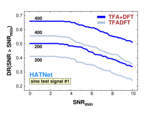
Figure 6: Detection ratio as a function of SNR for the sine test signal #1 of Table 1 on the HATNet sub-dataset. DR denotes the relative number of detections with SNR$>$SNR_min. The curves are labelled by the TFA template numbers. The partial time series models (blue lines with label tfa+dft) yield significantly higher detection rates than the full models (fainter lines with label tfadft).

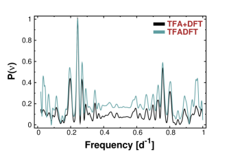
Figure 7: Example of the better performance of the partial time series model tfa+dft over the full model tfadft for the sine test signal (test signal #1 in Table 1). The spectra of one of the members of the $300$ objects used in this section for testing the HATNet database are shown. The number of TFA templates is equal to $400$. Both spectra are normalized to $1$ at the highest peak.

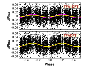
Figure 8: Folded light curves for the object with the frequency spectra shown in Fig. 7. The input sine signal is shown by pink line. The best single-component Fourier fit is overpolotted by yellow line. For better visibility, the data are plotted with twice of the test period. The partial time series model (upper panel) yields significantly lower amplitude fit in spite of finding the signal with a considerably higher significance than the full model search.

We exhibit the better detection capability of the partial model on one of the members of the testing set. Fig. 7 shows the frequency spectra for the two types of analysis. The higher variation of the spectrum away from the injected frequency in the case of full model results in an SNR of $9$, compared to $20$ of the partial model. Although the case displayed is characteristic of the more extreme examples, the SNR values of the full models rarely reach those of the partial models. This leads to the final accumulation of the higher detection ratio for the partial model, as shown in Fig. 6.

It is also interesting to examine the filtered time series resulting from the partial and full models. The folded time series, together with the input synthetic (noiseless) signals for the target above are shown in Fig. 8. We see that the application of the partial model leads to a substantial ($\sim 50$%) squeezing of the signal. This is because the partial model is based on the premise of the absence of an underlying signal and this may lead to fitting any variation in the time series that has some correlation with the TFA template set. For the same reason, the partial model treats true systematics better than the full model, because in the latter the flexible Fourier part of the fit may select the systematics as a real signal, when the wrong frequency is tested, thereby decreasing the fitting power of the TFA templates.

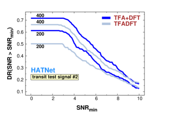
Figure 9: Detection ratio as a function of SNR for the transit test function (test signal #2 in Table 1). Notation is the same as in Fig. 6. The better detection capability of tfa+dft over tfadft is observable here too, albeit the effect is considerably smaller than for the sine test signal case.

The results of the same type of tests for the transit signal (test signal #2 in Table 1) are shown in Figs. 9,10 and 11. For the detection statistics a similar pattern to that of the sine test signal is observable, although the difference between the two methods is considerably smaller. This effect is likely due to the increased flexibility originating from the $10$-th order Fourier fit used to model the transit signal. This leads to higher false signal pick-up rates and a decrease in the importance of the better systematics filtering of the partial model. We expect that if the signal were modeled instead with a boxcar, which uses fewer parameters and is thus less flexible, then tfa+dft would provide an even greater enhancement over tfadft, closer to what was seen for the sinusoidal case.

The frequency spectra of a selected target (different from the one used in the sine test signal case) is shown in Fig. 10. The difference between the two methods is insignificant. The folded LCs (Fig. 11) are also similar but the decrease in the signal amplitude (i.e., transit depth) for the partial model is rather significant, similarly to the sinusoidal test signal case.

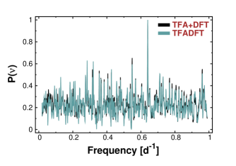
Figure 10: Example of the similar performance of the partial time series model tfa+dft and the full model tfadft for the transit-type test signal (test signal #2 in Table 1). A $10$-th order Fourier sum is used to search for the transit signal. Notation is the same as in Fig. 7

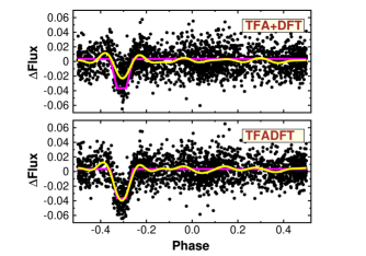
Figure 11: Folded light curves for the object with the frequency spectra shown in Fig. 10. The input trapezoidal transit signal is shown by pink line. The best $10$-th order Fourier fit is overpolotted by yellow line. The partial time series model (upper panel) yields shallower transit depth albeit both methods find the signal with the same significance.

Not only that the partial model detects signals with higher SNR, it also has the ability to detect the signal exclusively (i.e., when the full model prefers another frequency, which corresponds either to some systematics or some real signal present in the data in which the test signal is injected). We examine the mutually exclusive detections in the two types of models. Since these detections come into play usually at low SNR values, we pose only the frequency condition as the sole criterion for detection. The result for the two types of signal and different TFA template numbers are shown in Table 2.

We see that the partial model leads to significantly larger number of exclusive detections. However, two caveats should be mentioned here. First, most of the ‘detections’ have rather low SNR, leading to no detections in real applications. Roughly only one third of the exclusive detections for the partial models have SNR$>8$. For the full model the situation is worse and most of the exclusive detections have alias counterpart (with higher SNRs) in the partial model tests. Second, there might be also long-period variations in the stars, some of these variations could be intrinsic or long-term systematics. These might be preferred by the full model, leading to no detection of the injected signal. Whether or not these signals preferred by the full model are real, can be decided only by careful case-by-case studies, e.g., by running the analysis on varying TFA template numbers (Kovács & Bakos kovacs2007 (2007)), inspecting the light curves and checking other stars with similar periods. Our variable star works on various datasets show that the loss rate of long-period variables is small, and can be handled in the way mentioned (e.g., Dékány & Kovács dekany2009 (2009), Szulágyi, Kovács, & Welch szulagyi2009 (2009), Kovács et al. 2014).

Table 2: Mutually exclusive detections

Signal	$M$	$R_{\rm part}$	$R_{\rm full}$
$\#1$	200	0.111	0.020
	400	0.121	0.017
$\#2$	200	0.131	0.020
	400	0.077	0.024

Notes: $R_{\rm part}$ denotes the ratio of the number of exclusive detections in the partial (tfa+dft) model to the total number of objects tested (i.e., to $300$). Similarly, $R_{\rm full}$ refers to the same type of detections for tfadft. No SNR condition is posed.

3.4 Ensemble test: results based on K2

Most of the current works advocating simultaneous systematics filtering and signal search focus their attention on the data gathered by the K2 mission. Therefore (as suggested by the referee), it is of considerable importance to investigate if the overall better/similar performance of separate systematics filtering (tfa+dft) as indicated by the HATNet data survives also for the time series of the K2 mission. The selection procedure for the K2 test dataset has been described in Sect. 3.2.

Sinusoidal signal tests show quite clearly that unlike for the HATNet data, the detection rate is not a monotonic function of the TFA template number ($N_{\rm TFA}$) for the K2 data. Therefore, here we plot the detection rate as a function of $N_{\rm TFA}$ at a fixed lower bound of $SNR_{\rm min}=6$ for the SNR of the frequency spectra. (The relative topology of the detection rates is not affected in an essential way by changing $SNR_{\rm min}$ in both directions.)

The result for the sinusoidal test signal (#3 of Table 1) is shown in Fig. 12. The decrease of the detection rate (DR) both for the full-fledged and for the partial search is well exhibited. The full-fledged search have better statistics at the high $N_{\rm TFA}$ end but the downward trend for this type of search is also obvious. Before and shortly after the optimum detection rate, tfa+dft and tfadft behave similarly, with a slight preference toward higher detection rates for tfa+dft. This behavior is similar to what we found for the HATNet data.

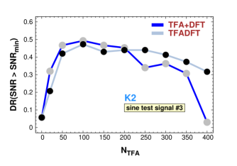
Figure 12: Detection ratio as a function of the number of the TFA templates for the injected sinusoidal test signal #3 (Table 1) in the subset of the K2/Campaign 1 data (see Sect. 3.2). Simultaneous systematics filtering and signal search (tfadft) performs somewhat poorer, except for higher template numbers, where the detection ratio saturates/decreases.

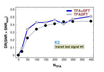
Figure 13: Detection ratio as a function of the number of the TFA templates for the injected transit test signal #4 (Table 1) in the subset of the K2/Campaign 1 data (see Sect. 3.2). Simultaneous systematics filtering and signal search (tfadft) performs poorer, except for higher template numbers, where the detection ratio saturates.

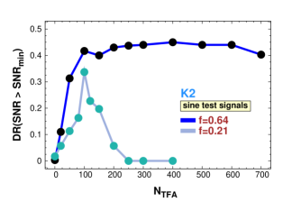
Figure 14: Testing the dependence of the detection ratio for injected sinusoidal signals in the K2 data. Test signals #5 and #6 of Table 1 are used in the ‘systematics filtering first, frequency search thereafter’ (tfa+dft) mode. The long period signal has a brief template range around $N_{\rm TFA}\sim 100$ where the detection ratio is optimal. The detection rate for the short period signal also saturates around this value but unlike the long period signal it remains around the optimum rate also for rather high TFA template numbers.

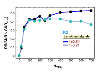
Figure 15: As in Fig. 14 but for the transit signals #4 and #7 of Table 1. Unlike the sinusoidal signals, transit signals remain optimally detected also for high TFA template numbers.

The detection rate for the transit signal (#4 of Table 1) shows a similar behavior in the low $N_{\rm TFA}$ regime (see Fig. 13). However, in the high $N_{\rm TFA}$ regime it behaves quite differently from the sinusoidal signal. The detection rate slightly increases for both search methods, a behavior observed both for the sinusoidal and for the transit test signals for the HATNet data. We conclude from these tests that, for the K2 data and for transit type signals, the partial model works similarly (or better) than the full-fledged model for a large range of TFA template numbers. For sinusoidal signals the same is true, except in the higher template regime, where the full-fledged method tends to outperform the partial model (albeit at a sub-optimal detection ratio).

Although the discussion and deeper testing of the non-monotonic nature of the detection rates for sinusoidal signals does not belong to the focus of this work, to have a somewhat better glimpse on the problem, we perform additional tests including the sinusoidal signals #5, #6 and transit signals #4, #7 of Table 1. (We note that these signals are constructed for testing the effect of the period, therefore, the same type of signals have the same amplitude/transit depth.) Since we aimed at testing CPU-demanding high template numbers, and the full-fledged search tend to yield similar results to the search based on the partial model, we restrict ourselves to the latter. Figs. 14, 15 confirm our earlier conclusion on the sensitivity of the detection rates of the sinusoidal signals on the template number and the insensitivity of the transit signals on the this parameter. However, it is important to note that for shorter signal periods the detection ratio for sinusoidal signals is significantly less sensitive to the number of TFA templates. Interestingly, the detection rates for transit type signals show fairly good stability even at higher template rates, although shorter period signals perform better (i.e., their detection rates tend to increase with the template number). Both for the sinusoidal and for the transit signal template numbers of $100$–$150$ yield close to optimum (maximal SNR) detection ratios. It is interesting to note that Foreman-Mackey et al. (foreman2015 (2015)) use similar number of eigen LCs from their PCA set derived on the Campaign 1 data.

Concerning the underlying cause of the depression of the detection rate for longer period sinusoidal signals, it is strongly suspected that the effect is attributed to the lower noise of the K2 data that enables the showing up of many physical variables among the template members (and obviously, the probability of picking up variables in the template set increases with the increase of the template numbers). The most likely impostors are the spotted variables, since they have close to sinusoidal light curves, cover a wide range of periods and some level of stellar activity is a generic property of main sequence stars (an observation, strongly supported by the recent discovery of a large number of rotational/spotted variables from the Kepler database – see McQuillan, Mazeh & Aigrain mcquillan2014 (2014)). For the HATNet data this is not a significant issue, since the noise floor for HATNet is higher, which blurs the physical signal for most of the low amplitude spotted stars. The fact that the transit signals have a much better survival rates also implies that most of the ‘signal killers’ are sinusoidal variables.

4 Conclusions

Identifying systematic effects in astronomical time series and correcting them without jeopardizing (but rather improving) the detection power of various signal search algorithms is a prime topic in contemporary efforts to find small transiting extrasolar planets and investigate low-amplitude stellar variability. Without knowing the exact time dependence of the systematics, we need to find the best method to disentangle the signal component from these, physically uninteresting effects. One obvious choice to retain both the signal content and, at the same time, filter out systematics, is to conduct a parameter search that includes both effects simultaneously. Although it is clear that at the end of any signal search one has to resort to a full model fit, it is unclear whether carrying out a full fit for systematics while searching for signals will not yield false detections due to the increased freedom in the fit. In particular, in the course of the frequency search, one has to try usually a huge number of cases. There might exist frequency bands, where a considerable part of the systematics is well approximated by the Fourier series or by some matched filter we use for the representation of the signal being searched for. In these cases the statistics used to construct the frequency spectrum might falsely indicate that there is a signal in that frequency band. Above all these, of course, there is also the computational deterrence in performing such a multiparametric search, primarily because of the strongly variable nature of the goodness of fit statistics on the test frequency.

In this paper we examined the performance of the frequency search methods based on full (systematics$+$signal) model fits. Four recent papers (Aigrain et al. aigrain2015 (2015); Foreman-Mackey et al. foreman2015 (2015); Angus et al. angus2015 (2015) and Wang et al. wang2015 (2015)) advocate this approach for the analysis of the photometric time series obtained by the K2 mission (the two reaction wheels program of the Kepler satellite). Because no counter tests with separately applied systematics filtering and signal search have been presented in those papers, we think it is important to execute such a test before we start a broader application of the full-fledged model method.

The tests presented in this paper (based on purely artificial data and signals injected in a sample of observed light curves from the HATNet project and from the Campaign 1 data of the K2 mission) clearly show that for signal search the partial model (systematics fitting only), is preferable over the full model search. This statement is based on the signal-to-noise ratio of the frequency spectra and tests performed on sinusoidal and transit-like periodic signals. For the HATNet data, the advantage of the partial model fit is especially visible for the sinusoidal test signals, where the detection rate is more than $10$% higher for the partial model. For transit-like signals this difference goes down to a few percent.

Because of the considerably lower noise level of the K2 data, the above conclusion should be expanded somewhat for signal shapes similar to those produced by intrinsic stellar variability (primarily by spot modulation due to stellar rotation). Depending on the period of the target, the detection ratio might decrease considerably for longer period sinusoidal signals for systematics filtering co-trending time series (template light curves) greater than $\sim 100$–$150$. With large template numbers the chance of finding intrinsic variables among them with periods close to that of the target, increases. This may lead to filtering out also the signal, not only the systematics. Transit signals are more robust in this respect, since similar quasi-coincidence with the co-trending template sample is far less likely. Although full-fledged search may prolong the survival rate somewhat in the regime of high template numbers, it does not lead to the detection of additional signals. The maximum detection rates resulting from the signal search based on partial time series modeling were never exceeded by the full-fledged models on any of the datasets tested.

Considering the possibility that a proper choice of basis (e.g., TFA template) functions and weighting of the signal and systematics parts of the model – based, e.g., on some more fundamental principles, such as the Bayesian inference – may still improve the situation for the full-fledged search, we add the following.

It is possible that a full-fledged method which includes a penalty for over-fitting the data, in particular which penalizes fitting periodic signals at frequencies where the systematics are found to have significant power and where the data would be equally well modeled using only the systematics filter, may have better performance at low S/N than the full-fledged method tested here. The filtering techniques presented, for example, by Roberts et al. (roberts2013 (2013)) or by Smith et al. (smith2012 (2012)) might be amenable to such an extension. Although we cannot predict the effect of the above extension of the full-fledged model on the effectiveness of the frequency search, based on the tests related to the subject of the paper we doubt that such a method would perform substantially better at low S/N than the two-step procedure.

Finally, the full model search is (obviously) always more time consuming, the one presented in this paper often by a factor of ten, depending slightly on the method of implementation. However, it is clear that in any period search influenced by systematics, the final step must be a full model fit (which is inexpensive). Once the signal is found, a full model fit will handle all constituents of the input time series properly and lead to the reconstruction of the signal by alleviating the effect of ‘signal squeezing’ caused by the partial model fit.

- (1) Aigrain, S., Hodgkin, S. T., Irwin, M. J., Lewis, J. R., & Roberts, S. J., 2015, MNRAS, 447, 2880
- (2) Alapini, A., & Aigrain, S., 2009, MNRAS, 397, 1591
- (3) Angus, R., Foreman-Mackey, D., & Johnson, J. A., 2015, arXiv1505.07105
- (4) Bakos, G. Á. et al., 2004, PASP, 116, 266
- (5) Bakos, G. Á. et al., 2010, ApJ, 710, 1724
- (6) Banachiewicz, T., 1937, Acta Astronomica, Series C, 3, 41
- (7) Berta, Z. K., Irwin, J., Charbonneau, D., Burke, C. J., & Falco, E. E., 2012, AJ, 144, 145
- (8) Chang, S.-W., Byun, Y.-I., & Hartman, J. D., 2015, AJ, 149, 135
- (9) Cubillos, P., Harrington, J., Madhusudhan, N. et al., 2014, ApJ, 797, 42
- (10) Dékány, I. & Kovács, G., 2009, A&A, 507, 803
- (11) Foreman-Mackey, D., Montet, B. T., Hogg, D. W. et al., 2015, ApJ, 806, 215
- (12) Honeycutt, R. K., 1992, PASP, 104, 435
- (13) Howell, S. B., Sobeck, C., Haas, M. et al., 2014, PASP, 126, 398
- (14) Huang, C. X., Penev, K., Hartman, J. D. et al., 2015, MNRAS, submitted, arXiv1507.07578
- (15) Kim, Dae-Won, Protopapas, P., Alcock, C., Byun, Yong-Ik, Bianco, F. B., 2009, MNRAS, 397, 558
- (16) Knutson, H. A., Charbonneau, D. A., Lori, E., Burrows, A., & Megeath, S. T., 2008, ApJ, 673, 526
- (17) Kovács, G., Zucker, S. & Mazeh, T. 2002, A&A, 391, 369
- (18) Kovács, G., Bakos, G., & Noyes, R. W., 2005, MNRAS, 356, 557
- (19) Kovács, G. & Bakos, G. Á., 2007, ASPC, 366, 133
- (20) Kovács, G. & Bakos, G. Á., 2008, CoAst, 157, 82
- (21) Kovács, G., Hartman, J. D., Bakos, G. Á. et al., 2014, MNRAS, 442, 2081
- (22) McQuillan, A., Mazeh, T., & Aigrain S., 2014, ApJS, 211, 24
- (23) Moutou, C., Pont, F., Barge, P. et al., 2005, A&A, 437, 355
- (24) Ofir, A., Alonso, R., Bonomo, A. S. et al., 2010, MNRAS, 404, L99
- (25) Petigura, E. A., & Marcy, G. W., 2012, PASP, 124, 1073
- (26) Press, W. H., Flannery, B. P., Teukolsky, S. A., & Vetterling, W. T., 1992, in ‘Numerical Recipes in FORTRAN: The Art of Scientific Computing, 2nd ed.’, Cambridge, England: Cambridge University Press
- (27) Rajan, M. P., & Mathew, J., 2012, Communications in Computer and Information Science, 305, 339
- (28) Rajpaul, V., Aigrain, S., Osborne, M. A., Reece, S., & Roberts, S. J., 2015, MNRAS, 452, 2269
- (29) Roberts, S., McQuillan, A., Reece, S., & Aigrain, S., 2013, MNRAS, 435, 3639
- (30) Samsing, J., 2015, ApJ, 807, 65
- (31) Smith, J. C., Stumpe, M. C., Van Cleve, J. E. et al., 2012, PASP, 124, 1000
- (32) Stumpe, M. C., Smith, J. C., Van Cleve, J. E. et al., 2012, PASP, 124, 985
- (33) Szulágyi, J., Kovács, G., & Welch, D. L., 2009, A&A, 500, 917
- (34) Tamuz, O., Mazeh, T., & Zucker, S., 2005, MNRAS, 356, 1466
- (35) Vanderburg, A. & Johnson, J. A., 2014, PASP, 126, 948
- (36) Wang, D., Foreman-Mackey, D., Hogg, D. W., & Schölkopf, B., 2015, arXiv1508.01853