Optimal growth trajectories with finite carrying capacity

Abstract

We consider the problem of finding optimal strategies that maximize the average growth-rate of multiplicative stochastic processes. For a geometric Brownian motion the problem is solved through the so-called Kelly criterion, according to which the optimal growth rate is achieved by investing a constant given fraction of resources at any step of the dynamics. We generalize these finding to the case of dynamical equations with finite carrying capacity, which can find applications in biology, mathematical ecology, and finance. We formulate the problem in terms of a stochastic process with multiplicative noise and a non-linear drift term that is determined by the specific functional form of carrying capacity. We solve the stochastic equation for two classes of carrying capacity functions (power laws and logarithmic), and in both cases compute optimal trajectories of the control parameter. We further test the validity of our analytical results using numerical simulations.  
 

I Introduction

There are many interesting connections between statistical mechanics and the theory of financial markets Geanakoplos1997 ; BouchaudPotters2000 . For instance, it has been stressed recently that the lack of ergodicity in the geometric Brownian motion process Peters1 has important implications for the optimal leverage problem, i.e. the problem of finding how much of a portfolio should be re-invested over time to maximize the logarithmic growth-rate of capital Peters2 .

For multiplicative processes, such as the geometric Brownian motion, the effective growth-rate is not given by the drift term alone. More precisely, consider the process described by

$$dK(t)=\rho K(t)(\mu dt+\sigma dW(t)),$$ (1)

with $\mu$ the drift of the stochastic process, $\sigma$ the noise amplitude, and $\rho$ a positive constant. Here $K(t)$ represents the capital of an investor at time t, while $\rho$ is the fraction of capital that is invested in a risky security, also known as the leverage. Using Ito’s formula it can be shown that $\left\langle dK(t)/K(t)\right\rangle=\mu\rho dt$, while $\left\langle d\log(K(t))\right\rangle=\rho(\mu-\frac{\sigma^{2}}{2})dt$, where $\langle\cdot\rangle$ represents the ensemble average over the stochastic process $dW(t)$. The fact that these two expected values are different has been interpreted in Peters2 ; Peters3 ; LauLubensky2007 as a characteristic signature of the absence of ergodicity, since the first expression can be identified as an ensemble average, while the second can be seen as the time average over an infinitely long single instance of the stochastic process.

In this context it has been argued that maximizing expected log-return of $ $K(t)$, often called the Kelly criterion Kelly1956 ; Kestner2003 ; Thorp2006 ; Breiman1961 ; opttrad1 ; opttrad2 ; CoverThomas1991 ; HanochLevy1969 , is a better objective in the long run than simply maximizing its average. For the case of the geometric Brownian motion, in Peters2 Peters discusses the differences between these two objectives, and provides a new interpretation of the optimal leverage obtained from the Kelly criterion by Thorp Thorp2006 , and shows that it is given by

$$\rho_{Thorp}=\frac{\mu}{\sigma^{2}}.$$ (2)

In this paper, we extend this analysis by computing optimal growth trajectories in the case of a multiplicative random process with finite carrying capacity, when the drift term $\hat{\mu}\equiv\mu(\rho K)$ is a decreasing function of $\rho(t)K(t)$. A finite carrying capacity can be associated with the presence of market frictions, such as transaction costs. Although we frame it in terms of investment decisions, our analysis is of interest beyond finance. For instance, stochastic processes with finite carrying capacity are commonly used in biology to describe the growth of a population constrained by a finite amount of resources and in a random environment. Stochastic Gompertzian differential equations are for instance well known in population ecology Kot , where one might want to control the amount or resources in order to optimize the growth of a population. This problem can be attacked using the methodology developed in this paper.

Below, we compute the optimal parameter $\rho(t)$ for logarithmic and power law functional forms of $\hat{\mu}\equiv\mu(\rho K)$. We will exactly solve the two models, and evaluate the optimal strategy, i.e. the parameter $\rho(t)$. In addition, we provide a methodology for evaluating the optimal control parameter $\rho(t)$ for generic series expansions of the carrying capacity parameter. Finally we show that numerical simulations agree with our analytical results.

II The model

Consider the following process: At time $t=0$, an investor has $K(0)=\$K_{0}$, and, at any discrete time step $t$, must decide the fraction $\rho(t)$ of her capital to invest in a risky asset. At the end of each period, the risky asset pays a return $r(t)$, which is drawn from a Gaussian distribution with average $\mu$ and standard deviation $\sigma$. Here we assume that there is a transaction cost $c(t)$ per dollar associated with the purchase of the risky asset, and that the asset purchased at time $t$ cannot be carried over to the next period, but needs to be sold at the end of each period. This is inspired by possible applications to wholesale electricity markets Wolak1 , in which trades have to be closed at the end of each trading day. Furthermore, we assume that the remaining fraction, $1-\rho(t)$, of the capital is not invested, and that its value does not change over the day (i.e., we assume the risk free interest rate is $0$ for simplicity).

Under the specifications above, the capital evolves between time $t$ and $t+1$ as:

$$K(t+1)=\left[(r(t)-c(t))\rho(t)+1\right]K(t).$$ (3)

If we are interested in the evolution of wealth over time horizons that are much longer than a trading period, we can consider the process in the limit of continuous time:

$$dK(t)=\rho(t)K(t)(r(t)-c(t)).$$ (4)

If we now assume that the returns evolve according to the stochastic process

$$r(t)=\mu dt+\sigma dW_{t},$$ (5)

and we define $c(t)=f\left(\frac{\rho(t)K(t)}{\tilde{K}}\right)dt$, we can write

$$\frac{dK(t)}{K(t)}=\rho(t)\hat{\mu}(\rho(t)K(t),t)dt+\rho(t)K(t)\sigma dW_{t},$$ (6)

where

$$\hat{\mu}(\rho(t)K(t),t)=\mu\left[1-f\left(\frac{\rho(t)K(t)}{\tilde{K}}\right)\right].$$ (7)

Here $\tilde{K}$ is the carrying capacity of the system, which in our context is associated with the cost of purchasing risky assets.

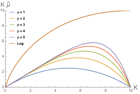
Figure 1: Return functional $K\hat{\mu}(K)$ of eqn. (LABEL:eqn:marketimpact), for $f(x)=x^{\gamma}$, with $\gamma=1,...,5$, and $f(x)=\log(x)$. The other constants are fixed at $\mu=\rho=1$, $\tilde{K}=10$, $\alpha=1$.

II.1 Analytical solution for $f(x)=x^{\gamma}$

In this section we solve the stochastic equation (6) in the case where $f(x)=x^{\gamma}$ and $\rho(t)=\rho$ is constant in time. We also use the simplifying assumption that the parameters $\mu$, $\sigma$ and $\gamma$ are constant in time. In this case we have that

$$\hat{\mu}(\rho K,t)=\mu\left(1-\left(\frac{\rho K}{\tilde{K}}\right)^{\gamma}\right),$$ (8)

where from now on we suppress the argument $t$ for the capital $K$. If we take $\rho=\tilde{K}=1$ we can write

$$dK=\mu K(1-K^{\gamma})dt+\sigma KdW_{t}.$$ (9)

Eqn. (9) can be solved using standard methods KloedenPlaten . Here we report only the solution for $\gamma=1$, but a full derivation for generic $\gamma$ can be found in Appendix A.1:

$$K(t) = \frac{\tilde{K}}{\rho}\ e^{(\rho\mu-\frac{(\rho\sigma)^{2}}{2})t+\rho\sigma W_{t}}$$

$$\times \left(\frac{\tilde{K}}{\rho K_{0}}+\rho\mu\int_{0}^{t}e^{(\rho\mu-\frac{(\rho\sigma)^{2}}{2})s+\rho\sigma W_{s}}ds\right)^{-1}.$$

The asymptotic stochastic equilibrium of the above solution can be determined by solving

$$\langle d\log(K(t)/K_{0})\rangle=0.$$ (11)

In fact, from eqn. (6) and using Itô theorem, we obtain

$$0=\langle d\log(K/K_{0})\rangle=\rho(t)\mu\left(1-f\left(\frac{\rho(t)K(t)}{\tilde{K}}\right)\right)-\frac{\sigma^{2}}{2}\rho^{2}$$ (12)

and for linear functions $f(\cdot)$ we obtain $K=\tilde{K}(\frac{1}{\rho}-\frac{\sigma^{2}}{2\mu})=\tilde{K}(\frac{1}{\rho}-\frac{1}{2\rho_{Thorp}})$. If the parameter $\rho$ is constant, the above implies an asymptotic equilibrium state $K(\infty)$. This equilibrium point is compatible with our simulations presented in the following.. This also holds in the case of the geometrical Brownian motion, where $\rho_{opt}\equiv\rho_{Thorp}=\frac{\mu}{\sigma^{2}}$ was computed in Thorp2006 ; Peters2 .

II.2 Analytical solution for $f(x)=\alpha\log(x)$

In this section we provide a solution for the logarithmic functional form of carrying capacity, introduced recently in Marketimpact2 for the case of stock markets and describing cell growth. The equation of interest is

$$dK=\mu K\left(1-\alpha\log\left(\frac{K}{\tilde{K}}\right)\right)dt+\sigma\ K\ dW_{t},$$ (13)

for the case where $\rho$ is constant. The solution is obtained in Appendix A.2, where we find:

$$K(t) = \exp\left[e^{-\alpha\mu t}\left(C_{0}+\left(\mu(1+\alpha\log(\tilde{K}))-\frac{\sigma^{2}}{2}\right)\frac{e^{\alpha\mu t}-1}{\alpha\mu}+\sigma\int_{0}^{t}e^{\alpha\mu s}dW_{s}\right)\right]$$ (14)

The expectation $\left\langle\log(K(t))\right\rangle$ can then be evaluated analytically, using $\left\langle\int_{0}^{t}f(s)dW_{s}\right\rangle=0$ for any deterministic and continuous function $f(s)$, and thus, substituting $C_{0}=\log(K_{0})$,

$$\left\langle\log(K(t))\right\rangle = e^{-\alpha\mu t}\left(C_{0}+\left(\left(\frac{1}{\alpha}+\log(\tilde{K})\right)-\frac{\sigma^{2}}{2\alpha\mu}\right)(e^{\alpha\mu t}-1)\right).$$

Looking at the asymptotic stochastic equilibrium point again, we have

$$\left\langle\log(K(t\rightarrow\infty))\right\rangle = \log(\tilde{K})+{\frac{1}{\alpha}\left(1-\frac{\sigma^{2}}{2\mu}\right)}.$$

We note that while the expected return and the exponential of expected log-return are not equal, they converge asymptotically.

III Optimal trajectories

We now turn to the problem of finding the optimal trajectory $\rho(t)$ following the Kelly strategy that maximizes the expected log-return of the investor’s capital, i.e., $\left\langle\log(K(t)/K_{0})\right\rangle$. In general, we must solve the equation

$$d\log(\frac{K}{K_{0}}) = \left[\mu\rho(t)\left(1-f\left(\frac{\rho(t)K(t)}{\tilde{K}}\right)\right)-\rho^{2}(t)\frac{\sigma^{2}}{2}\right]dt$$ (17)

$$+ \rho(t)\sigma dW_{t},$$

which implies

$$\left\langle d\log(\frac{K}{K_{0}})\right\rangle = \left\langle\mu\rho(t)\left(1-f\left(\frac{\rho(t)K(t)}{\tilde{K}}\right)\right)-\rho^{2}(t)\frac{\sigma^{2}}{2}\right\rangle dt$$ (18)

$$+ \left\langle\rho(t)\sigma dW_{t}\right\rangle.$$

It is instructive to discuss first the case of a time-dependent $\rho$ in eqn. (18), and then provide approximations for which we can obtain an explicit solution for the optimal parameter $\rho$. Using (18), the expected logarithmic return over a time horizon $T$ is:

$$\log\left(\frac{K(T)}{K_{0}}\right)=$$

$$\int_{0}^{T}\left\langle\mu\rho(t)\left(1-f\left(\frac{\rho(t)K(t)}{\tilde{K}}\right)\right)-\rho^{2}(t)\frac{\sigma^{2}}{2}\right\rangle dt.$$ (19)

The main difference with respect to the case of no carrying capacity is the fact that due to the effective dependence of the drift term on $K$, optimizing eqn. (19) requires taking a functional derivative with respect to $\rho(t)$ and setting it to zero, i.e.,

$$\frac{\delta}{\delta\rho(t)}\log\left(\frac{K(T)}{K_{0}}\right)=0\,.$$ (20)

In the case of a pure geometric Brownian motion, it can be shown that the optimal $\rho(t)$ is constant in time. In the case under consideration one strategy is to first obtain a solution for arbitrary $\rho(t)$, and then take the functional derivative in the integral of eqn. $(\ref{eq:max})$. Unfortunately, this is difficult, so in the following we will resort to two different approximations. First we take the stationary case, in which the solution for constant $\rho$ is known, as discussed in Sec. III.1. For the second approximation, if we write the function of the carrying capacity as a series expansion, we can write a dynamical set of equations for the derivatives of all the moments of the solution $\left\langle K(t)^{n}\right\rangle$ which then can be optimized iteratively; this procedure will be discussed in Sec. III.2.

III.1 Stationary approximation

In this section we will use the exact solutions obtained in Sec. II.1 and Sec. II.2 under the assumption of constant parameter $\rho$ within a quasi-stationary approximation scheme. More precisely, we assume that $\rho(t)$ is a slow variable with respect to $K(t)$, and that the latter quickly relaxes to what would be its asymptotic value should $\rho$ remain constant. The validity of the approximation can then be assessed from the obtained solution by checking whether $|\left\langle K(t)\right\rangle\frac{\partial_{t}\rho(t)}{\partial_{t}\left\langle K(t)\right\rangle}|\ll 1$.

In general, we have that

$$\frac{\delta}{\delta\rho(t)}\log\left(\frac{K(T)}{K_{0}}\right)$$ (21)

$$= \frac{\delta}{\delta\rho(t)}\int_{0}^{T}\left[\mu\rho(t)\left(1-\left\langle f\left(\rho(t)\frac{K(t)}{\tilde{K}}\right)\right\rangle\right)-\rho^{2}(t)\frac{\sigma^{2}}{2}\right]dt$$

$$= \int_{0}^{T}\left[\mu\left(1-f\left(\rho(t)\frac{K(t)}{\tilde{K}}\right)\right)-2\rho(t)\frac{\sigma^{2}}{2}\right.$$

$$- \left.\rho(t)\mu\frac{\delta}{\delta\rho(t)}\left\langle f\left(\rho(t)\frac{K(t)}{\tilde{K}}\right)\right\rangle\right]dt.$$

To find an optimal solution, we now impose the following condition:

$$\mu \left(1-f\left(\rho(t)\frac{K(t)}{\tilde{K}}\right)\right)-2\rho(t)\frac{\sigma^{2}}{2}$$

$$- \rho(t)\mu\frac{\delta}{\delta\rho(t)}\left\langle f\left(\rho(t)\frac{K(t)}{\tilde{K}}\right)\right\rangle=0,$$

where the last functional derivative requires knowledge of $K(\rho(t),t)$ for arbitrary $\rho(t)$. In order to evaluate this functional derivative, as a first approximation, we will assume that $\rho(t)\approx\rho$ in the interval $\Theta=[t,t+\delta t]$. If this is true, then we can evolve in the interval $\Theta$ the solution with a constant $\rho$ from $t_{0}=t$ to $t_{f}=t+\delta t$ with initial condition $K_{0}=K(t)$. Let us call such a solution $\mathcal{K}(\delta t,\rho,K(t))$, which satisfies the property $\lim_{\delta t\rightarrow 0}\mathcal{K}(\delta t,\rho,K(t))=K(t)$. The underlying assumption of this approach is that $\rho(t)$ changes slowly with respect to the stochastic dynamics, which implies that $|\left\langle K(t)\right\rangle\frac{\partial_{t}\rho(t)}{\partial_{t}\left\langle K(t)\right\rangle}|\ll 1$. Within this approximation, we can write the functional derivative as:

$$\frac{\delta}{\delta\rho(t)}\left\langle f\left(\rho(t)\frac{K(t)}{\tilde{K}}\right)\right\rangle\approx\partial_{\rho}\left\langle f\left(\rho\frac{\mathcal{K}(t+\delta t,\rho,K(t))}{\tilde{K}}\right)\right\rangle,$$ (23)

Then the optimal instantaneous parameter $\rho(t)$ can be obtained by solving the following equation:

$$\mu\left(1-f\left(\rho(t)\frac{K(t)}{\tilde{K}}\right)\right)-2\rho(t)\frac{\sigma^{2}}{2}=\lim_{\delta t\rightarrow 0}\rho(t)\mu\ \partial_{\rho}\left\langle f\left(\rho(t)\frac{\mathcal{K}(\delta t,\rho,K(t))}{\tilde{K}}\right)\right\rangle,$$ (24)

which is the approximation we use in the following.

III.1.1 $f(x)=x^{\gamma}$: Expansion assuming $\frac{K}{\tilde{K}}\ll 1$

In the case of $f(x)=x^{\gamma}$, evaluating $\left\langle f\right\rangle$ is a non trivial task. Even assuming we have the stationary approximation, expanding equation (52) in $K/\tilde{K}$, and considering only the zeroth order term of this expansion, we obtain the following expression to be solved for $\rho$,

$$\mu\left(1-\left(\frac{K\rho}{\tilde{K}}\right)^{\gamma}\right)-\rho\sigma^{2}=0,$$ (25)

which cannot be solved analytically for arbitrary values of $\gamma$. However, for $K\gg\tilde{K}$, we can obtain the approximate solution

$$\rho(K\gg\tilde{K})\approx\frac{\tilde{K}}{K},$$ (26)

which is independent of $\gamma$. A plot with the numerical solutions of $\rho(K)$ obtained from (25) for different values of $\gamma$ is shown in Fig. 2.

In the particular case of $\gamma=1$ the solution is simply:

$$\rho(t)=\frac{\mu}{2\mu\frac{K(t)}{\tilde{K}}+\sigma^{2}},$$ (27)

which shows explicitly that the presence of carrying capacity effectively increases the risk, as the optimal fraction of resources to be deployed is a decreasing function of $K$. This is important as is it a generalization of the result of Peters1 and has direct applications to the problem of optimal trajectories in the context of financial time series where one has an embedded transaction cost. This applies for instance to lotteries and wholesale electricity markets, where one has independent processes at each time step. In this case, the transaction cost plays the role of market impact.

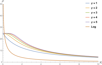
Figure 2: Optimal parameter $\rho(t)$ obtained numerically from eqn. (25) as a function of $K\in[0,10]$, for various values of $\gamma$, and for logarithmic carrying capacity with $\alpha=1$. Other constants are fixed at $\mu=1$, $\sigma=0.2$, $\tilde{K}=50$.

Surprisingly, the optimal parameter of eqn. (27) holds up to second order in $\xi=\frac{K}{\tilde{K}}$. In order to obtain precise estimates of the parameter $\rho$, the expectation $\left\langle K\right\rangle$ must be evaluated. This is done up to second order in $\xi$ in Appendix B, using techniques partly developed in Caravellietal .

In order to check the consistency of the stationarity approximation, we evaluate

$$\partial_{t}\rho(t)=\partial_{t}\frac{\mu}{2\frac{K(t)}{\tilde{K}}+\sigma^{2}}=-\frac{\mu}{(2\frac{K(t)}{\tilde{K}}+\sigma^{2})^{2}}\left(2\frac{\partial_{t}K(t)}{\tilde{K}}\right),$$ (28)

which implies

$$\left|\frac{\partial_{t}\rho(t)}{\frac{\partial_{t}K(t)}{K(t)}}\right|=\frac{2\mu}{\left(2\frac{K(t)}{\tilde{K}}+\sigma^{2}\right)^{2}}\frac{K(t)}{\tilde{K}}.$$ (29)

The right hand side of eqn. (29) is small as long as $\frac{K(t)}{\tilde{K}}\ll 1$, consistent with the expansion we performed.

Next we take the optimal $\rho(t)$ from above, and study the implied stochastic differential equation for $K(t)$. For the case of $\gamma=1$ we have:

$$d\log(K/K_{0})=\frac{1}{2}\frac{\mu^{2}}{2\mu\frac{K}{\tilde{K}}+\sigma^{2}}dt+\frac{\mu\sigma}{2\mu\frac{K}{\tilde{K}}+\sigma^{2}}dW.$$ (30)

When $K\gg\frac{\sigma^{2}\tilde{K}}{\mu}$, this simplifies to:

$$\langle d\log(K/K_{0})\rangle=\frac{1}{4}\frac{\mu\tilde{K}}{K}dt.$$ (31)

Since we observe that the asymptotic growth is compatible with a linear function of $K$, we can obtain the proportionality constant by using the ansatz $K(T)\approx aT$, we obtain that the slope of the linear approximation is $\frac{\mu\tilde{K}}{4}$ for $T\gg\frac{\sigma^{2}}{4\mu^{2}}$. Further, when $\tilde{K}\rightarrow\infty$, this slope $\rightarrow\infty$ as well, because we are asymptotically approximating an exponential with a linear function.

III.1.2 $f(x)=\alpha\log(x)$

For the case of a logarithmic carrying capacity term we have shown how to evaluate explicitly $\left\langle K(t)\right\rangle$ and $\left\langle\log(K(t))\right\rangle$ in eqns. (LABEL:eqn:logav). Using this solution, if we assume the stationary approximation in which $\rho$ changes slowly compared to $K$, we obtain the following equation for the optimal parameter $\rho$ in the limit $\delta t\to 0$:

$$\alpha\mu\left(\log\left(\frac{\tilde{K}}{\rho}\right)-\log(\text{K(t)}/K_{0})\right)+\mu(1-\alpha)-\rho\sigma^{2}=0,$$ (32)

from which we can solve for $\rho(t)$:

$$\rho_{opt}(t)\approx\alpha W\left(\frac{K_{0}e^{\frac{1}{\alpha}-1}\tilde{K}\sigma^{2}}{\alpha K(t)\mu}\right)\frac{\mu}{\sigma^{2}},$$ (33)

where $W$ is the Lambert W-function. Note that for $\alpha\rightarrow 0$ we recover again the result of Peters1 . This allows us to evaluate the critical ratio $\xi=\frac{K}{\tilde{K}}$ for which $\rho_{opt}=1$, which is given by $\xi=e^{\frac{1}{\alpha}(\frac{\sigma^{2}}{\mu}-1)-1}$.

Similarly to the case of a linear carrying capacity given in eqn. (30), we can obtain an effective differential equation by inserting the obtained optimal $\rho(t)$ of eqn. (33). Using the asymptotic properties of the Lambert W-function in the limit $K\gg 1$, this differential equation is given by

$$\left\langle d\log(K)\right\rangle\approx\tilde{K}\mu dt,$$ (34)

which implies an asymptotic linear growth given by $K(T)\approx 4aT$, where $a=\frac{\mu\tilde{K}}{4}$ is the slope obtained in eqn. (31). We thus have the result that in the case of logarithmic carrying capacity, the Kelly strategy implies a growth rate which is asymptotically twice the rate obtained for a linear function.

III.2 Analytical result: short timescales

The approach of the previous section has some drawbacks, in particular, evaluating cumulants of the exponential of the Brownian motion is a lengthy task in general. While for the case of logarithmic carrying capacity it is possible to evaluate the averages exactly, this is not true in the general case. As an alternative, we can proceed by directly integrating the equations for the moments and elaborating an approximation scheme based on the smallness of the time horizon with respect to the other scales.

It is reasonable to expect that at least for small variations the carrying capacity can be parametrized with a power series, leading to the following stochastic differential equation:

$$dK=\rho\mu K\left(1+\sum_{k=1}^{n}\lambda_{k}(\rho K)^{k\gamma}\right)dt+\sigma\rho KdW.$$ (35)

As before, we focus on the maximization of the expectation value of the logarithm of $K$. Using Ito’s Lemma,

$$\left\langle\frac{d}{dt}\log K/K_{0}\right\rangle=\mu\rho\left(1+{\sum_{k=1}^{n}\lambda_{k}\rho^{k\gamma}\left\langle K^{k\gamma}\right\rangle}\right)-\frac{\sigma^{2}\rho^{2}}{2}\,.$$ (36)

To solve this equation for generic values of the parameters $\lambda_{k}$, we need to compute all the moments $\langle K^{m\gamma}\rangle$, that is, we need to solve the equations of motion for these observables:

$$\left\langle\frac{d}{dt}K^{m\gamma}\right\rangle=\mu\rho\gamma m\left\langle\left(1+\sum_{k=1}^{n}\lambda_{k}\rho^{k\gamma}K^{k\gamma}\right)K^{m\gamma}\right\rangle$$

$$+\ \gamma m(\gamma m-1)\frac{\sigma^{2}\rho^{2}}{2}\left\langle K^{m\gamma}\right\rangle.$$ (37)

These form a tower of coupled equations. Using the notation $e_{m}:=\left\langle K^{m\gamma}\right\rangle$, we can write the above as:

$$\dot{e}_{m}=\mu\rho\gamma m\sum_{k=0}^{n}\lambda_{k}\rho^{k\gamma}e_{m+k}+\\ \gamma m(\gamma m-1)\frac{\sigma^{2}\rho^{2}}{2}e_{m},$$ (38)

where $\lambda_{0}=1$. The initial conditions are $e_{m}(t_{0})=K_{0}^{\gamma m}$, as the PDF for $K(t=t_{0})$ is a Dirac delta at the initial time.

With these equations, given a time horizon $\delta t$, we can compute the Taylor expansion of the derivative $d\log K(t)/dt$ at any order in an expansion in $\delta t$. In general, this is given by:

$$\frac{d}{dt}\log(K(t_{0}+\delta t))=\Phi(K_{0},\mu,\sigma,\gamma,\{\lambda_{k}\};\delta t),$$ (39)

with

$$\Phi(K_{0},\mu,\sigma,\gamma,\{\lambda_{k}=\delta_{k}^{0}\};\delta t)=\mu\rho-\frac{{\sigma}^{2}\rho^{2}}{2}.$$ (40)

Using this general procedure, the maximisation needed to determine $\rho$ is straightforward, once a truncation in the expansion in $\delta t$ has been fixed. As an example, consider the case in which

$$\gamma=1,\qquad n=1,\qquad\lambda_{1}=-\frac{1}{\tilde{K}}.$$ (41)

To first order in $\delta t$ we then have:

$$\left\langle\frac{d}{dt}\log K\right\rangle\simeq\mu\rho-\frac{\rho^{2}\sigma^{2}}{2}+$$

$$-\frac{{K_{0}}\mu\rho^{2}}{\tilde{K}}+\left(\frac{K_{0}^{2}\mu^{2}\rho^{4}}{{\tilde{K}}^{2}}-\frac{K_{0}\mu^{2}\rho^{3}}{{\tilde{K}}}\right)\delta t\,.$$ (42)

As expected, the corrections to the geometric Brownian motion case are controlled by the quantity ${\frac{K_{0}}{\tilde{K}}}$. With respect to these quantities, the optimal parameter $\rho$ is:

$$\rho_{opt}\simeq\frac{\mu}{2\mu\frac{K_{0}}{\tilde{K}}+\sigma^{2}}+\frac{\left(-3{\tilde{K}}^{3}\mu^{4}\sigma^{2}K_{0}-2{\tilde{K}}^{2}\mu^{5}K_{0}^{2}\right)}{\left(2\mu K_{0}+\tilde{K}\sigma^{2}\right)^{4}}\delta t.$$ (43)

In this last expression we recognize, at the zeroth order, the same term obtained in the approximation in which $\rho(t)$ is constant. At the first order we obtain a correction proportional to the size of the time horizon $\delta t$. These results can be generalized without difficulty to higher orders.

What is remarkable in the result of this short timescale analysis is that the optimal value for $\rho$, in the general case, is a function of the initial condition, the parameters of the process and of the time horizon.

III.3 Numerical simulations

In this section we present numerical tests of our analytical results, using a Monte Carlo approach and a stochastic Euler method to solve the differential equations.

First, In Fig. 3 we report the expectation values of log returns over a fixed time horizon $T=1$ and for different values of the parameter $\rho$, assumed to be constant in time, and for different values for the scale of carrying capacity. Each point is an estimate for the expectation of the endpoint of the numerical solution of the corresponding stochastic differential equation. The curves that are obtained from these points clarify how the log returns reach their maximum for special choices of $\rho$. The points on the upper curve are obtained in the case of no dependence on the amount of resources, i.e., the simple geometric Brownian motion. They match the results of Peters1 for the values of the parameters that we are considering. As expected, the plot shows that the optimal $\rho$ decreases with the strength of carrying capacity.

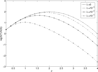
Figure 3: Log return as a function of $\rho$ at $T=1$ for parameters $K(0)=1$, $\mu=2$, $\sigma=1$, $\gamma=1$ and various values of $\lambda=1/\tilde{K}$.

In Fig. 4 we use eqn. (43) at zeroth order and compare to the strategy at constant $\rho=1$. We can see that the dynamic strategy outperforms those which are kept constant, and that it works reasonably well also in the case in which $K(t)\approx\tilde{K}$. In Fig. 5 we compare this result with the first order approximation in $\delta t$. In the inset we see that the latter outperforms the optimal solution obtained at zeroth order, although the difference between the two is overall relatively small. For $\gamma\neq 1$, our solution also outperforms the constant solution.

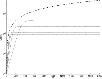
Figure 4: Optimal Kelly path for $K$ with carrying capacity function $x^{\gamma}$ plotted against the case of those fixed at $\rho=1,0.8,0.6,0.4,$ and $0.2$ (full lines).The parameters used are $K(0)=1$, $dt=0.01$, $\mu=0.1$, $\sigma=0.1$, $\tilde{K}=10$ and $\gamma=1$, averaged over $2000$ samples. The horizontal dashed lines represents the stochastic equilibria obtained from the analytic formula.

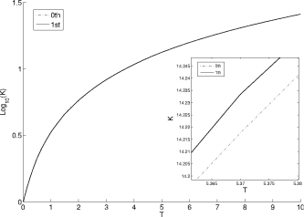
Figure 5: Expected value of $K$ for the case of power law carrying capacity, with the optimal parameter $\rho$ evaluated using the 0th order in the time horizon (dashed) and 1st (solid) order correction, for $K_{0}=1$, $\tilde{K}=100$, $dt=0.01$, $\sigma=0.2$, $\mu=1$ and $\gamma=1$. In order to distinguish the two curves, we averaged over 1000 Monte Carlo runs. We observe that the solution obtained at the first order outperforms the one obtained at the zeroth order.

For logarithmic carrying capacity, we can see in Fig. 6 that our optimal parameter $\rho(t)$ solution again outperforms the constant solution. Also note that the stochastic equilibrium obtained from eqn. (11) is confirmed both in Fig. 4 and Fig. 6.

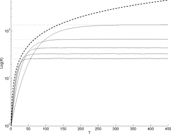
Figure 6: Optimal Kelly time path of $K$ for logarithmic carrying capacity compared to the case of those fixed at $\rho=1,0.8,0.6,0.4,$ and $0.2$ (full lines).The parameters used were $K(0)=1$, $dt=0.01$, $\mu=0.1$, $\sigma=0.1$, $\tilde{K}=10$ and $\gamma=1$, averaged over $2000$ samples. The horizontal dashed lines represents the stochastic equilibria obtained from the analytic formula.

Finally in Fig. 7 we compare the linear regimes for the case of linear and logarithmic carrying capacity obtained in eqns. (31) and (34) to the curves obtained with Monte-Carlo simulations, showing that the slopes obtained analytically are a good match with the numerical ones.

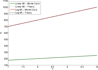
Figure 7: Average asymptotic ($T\approx 7$) linear regime in the case of linear (green curve) and logarithmic (red curve) carrying capacity for the case of $\sigma=0.2$, $\mu=1$ and $\tilde{K}=10$ obtained using a Monte Carlo averaged over 2000 samples, with integration step $dt=0.01$. The dashed lines represent the comparison with the linear coefficients obtained from theory, eqns. (31) and (34).

IV Conclusions

In this paper we computed optimal strategies for the problem of maximal growth using the Kelly criterion, in the case of a drift term which represents the presence of carrying capacity. Using two different methods, one considering exact solutions at constant leverage, and the second solving for the optimal solution at fixed time horizon, we obtained the same result at the lowest order. Our solutions were also tested numerically, confirming that these are optimal as compared to the case in which carrying capacity is ignored.

We considered two specific carrying capacity functions for which empirical evidence has been presented in the literature Marketimpact1 ; Marketimpact2 : a power law and a logarithmic function. In the case of a power law carrying capacity function, we have shown that in order to evaluate the optimal solution various approximations have to be used, but we have shown that the zeroth order is correct up to second order in the parameter controlling the scale of the carrying capacity, and provided a solution up to first order for the case of a finite time horizon. In the case of a logarithmic carrying capacity function, expectations can be evaluated exactly.

The main difference between the case of the geometric Brownian motion and the case with carrying capacity is that the former requires a constant leverage while in the latter the leverage has to be dynamically adapted. The operator has to adapt his strategy continuously depending on his position with respect to the capacity parameter. Our results support this intuitive observation and, at the same time, complement it with concrete procedures for quantitative estimates.

Finally, the analysis presented heavily relies on the Gaussian nature of the noise term and on the powerful results of Ito’s calculus. Our results can then be seen as a first assessment of the effects of carrying capacity on investment strategies, which, however, will require further elaboration. In particular, a natural extension will be the inclusion of more realistic noise terms, like general Levy processes. The investigation of the impact of a more detailed noise structure on the optimal leverage will be the subject of future work.

Appendix A Solution of the stochastic differential equations for constant $\rho$

A.1 Power law function

In this Appendix we discuss the solution of the equation:

$$dK=\mu K(1-K^{\gamma})dt+\sigma KdW_{t}.$$ (44)

Using the change of variables $y=K^{-\gamma}$ and Ito’s Lemma, we have:

$$dy=\left(-\gamma\mu(y-1)+\frac{\sigma^{2}\gamma(\gamma+1)}{2}y\right)dt-\gamma\sigma ydW_{t}.$$ (45)

Notice that eqn. (45) is a stochastic differential equation of the form:

$$dz=(az+c)dt+(bz+d)dW,$$ (46)

where

$$a = \frac{\sigma^{2}\gamma(\gamma+1)}{2}-\gamma\mu$$

$$b = -\sigma\gamma$$

$$c = \gamma\mu$$

$$d = 0.$$ (47)

This is an inhomogeneous linear stochastic differential equation with multiplicative noise KloedenPlaten , and has a known solution. If we define

$$\Phi_{t} \equiv \exp\left((a-b^{2}/2)t+bW_{t}\right)$$

$$\rightarrow\Phi_{t} = \exp\left(-(\mu-\sigma^{2}/2)t-\sigma W_{t}\right),$$ (48)

the solution is then given by

$$z=\Phi_{t}\left(z_{0}+(c-bd)\int_{0}^{t}\Phi_{s}^{-1}ds+d\int_{0}^{t}\Phi_{s}^{-1}dW_{s}\right).$$ (49)

Writing

$$f_{t}(a,b,c,z_{0})=\Phi_{t}\left(z_{0}+c\int_{0}^{t}\Phi_{s}^{-1}ds\right),$$ (50)

we obtain

$$y(t)=f_{t}\left(-\gamma\mu+\frac{\sigma^{2}\gamma(\gamma+1)}{2},-\gamma\sigma,\gamma b,y_{0}\right).$$ (51)

Going back to the variable $K(t)$, we have

$$K(t)=\left[f_{t}\left(-\gamma\mu+\frac{\sigma^{2}\gamma(\gamma+1)}{2},-\gamma\sigma,\gamma b,y_{0}\right)\right]^{-1/\gamma}.$$ (52)

If we examine the special case of $\gamma=1$, and insert again the constants $\rho$ and $\tilde{K}$ by rescaling $\mu\rightarrow\rho\mu$ and $\sigma\rightarrow\rho\sigma$, $\tilde{K}\rightarrow\tilde{K}/\rho$, we obtain the full solution in terms of all the original parameters:

$$K(t) = \frac{\tilde{K}}{\rho}\ e^{(\rho\mu-\frac{(\rho\sigma)^{2}}{2})t+\rho\sigma W_{t}}$$

$$\times \left(\frac{\tilde{K}}{\rho K_{0}}+\rho\mu\int_{0}^{t}e^{(\rho\mu-\frac{(\rho\sigma)^{2}}{2})s+\rho\sigma W_{s}}ds\right)^{-1},$$

which is the solution used in this paper in the case of a power law carrying capacity.

A.2 Logarithmic function

In the case of a logarithmic carrying capacity function, and again if $\rho(t)=\rho=1$, we have the following differential:

$$dK=\mu K\left(1-\alpha\log\left(\frac{K}{\tilde{K}}\right)\right)dt+\sigma\ K\ dW_{t},$$ (54)

which is a stochastic Gompertzian-type of equation Gompertz ; Ferrante2000 ; Lo2009 . Such equation for instance appear also in the growth of reproducing cells, where now $\tilde{K}/\rho(t)$ represents the amount of nutrient accessible to the cells. This implies that there is a parallel between optimal leverage trajectories and optimal cell growth. If we change variables to $y=\log(K)$, then through Ito’s Lemma the above becomes:

$$dy=\left[\mu\left(1-\alpha y+\alpha\log(\tilde{K})\right)-\frac{\sigma^{2}}{2}\right]dt+\sigma\ dW_{t}.$$ (55)

This has the same form as eqn. (46) in the previous section, with:

$$a = -\alpha\mu$$

$$b = 0$$

$$c = \mu(1+\alpha\log(\tilde{K}))-\frac{\sigma^{2}}{2}$$

$$d = \sigma.$$ (56)

We then have that

$$\Phi_{t}=\exp\left(-\alpha\mu t\right),$$ (57)

and thus one obtains

$$K(t) = \exp\left[e^{-\alpha\mu t}\left(C_{0}+\left(\mu(1+\alpha\log(\tilde{K}))-\frac{\sigma^{2}}{2}\right)\int_{0}^{t}e^{\alpha\mu s}ds+\sigma\int_{0}^{t}e^{\alpha\mu s}dW_{s}\right)\right]$$ (58)

$$= \exp\left[e^{-\alpha\mu t}\left(C_{0}+\left(\mu(1+\alpha\log(\tilde{K}))-\frac{\sigma^{2}}{2}\right)\frac{e^{\alpha\mu t}-1}{\alpha\mu}+\sigma\int_{0}^{t}e^{\alpha\mu s}dW_{s}\right)\right]$$

Appendix B Average $\left\langle K\right\rangle$ for $f(x)=x$

In this appendix we evaluate the average $\left\langle K\right\rangle$ as an expansion of $\xi=\frac{K}{\tilde{K}}$ of the denominator of the solution in eqn. (II.1), and show that the optimal leverage obtained in eqn. (27) holds up to second order in $\xi$. For simplicity, we will set $\rho=1$ during the calculation of the averages, and then restore $\rho\neq 1$ by rescaling $\sigma\rightarrow\rho\sigma$, $\mu\rightarrow\rho\mu$ and $\tilde{K}\rightarrow\tilde{K}/\rho$. In this case, expanding (A.1) to order $\left(K(t)/\tilde{K}\right)^{2}$ we have that

$$\mathcal{K}(\delta t,\rho=1,K(t))) =$$

$$\tilde{K}\ e^{(\mu-\frac{\sigma^{2}}{2})\delta t+\sigma W_{\delta t}}\left(\frac{\tilde{K}}{K(t)}+\mu\int_{0}^{\delta t}e^{(\mu-\frac{\sigma^{2}}{2})s+\sigma W_{s}}ds\right)^{-1} \approx$$

$$K(t)\ e^{(\mu-\frac{\sigma^{2}}{2})\delta t+\sigma W_{\delta t}}\left(1-\frac{\mu K(t)}{\tilde{K}}\int_{0}^{\delta t}e^{(\mu-\frac{\sigma^{2}}{2})s+\sigma W_{s}}ds\right).$$ (59)

Taking the expectation of the above, we have:

$$\left\langle\mathcal{K}\right\rangle=\left\langle K_{\tilde{K}=\infty}(t)\right\rangle-\frac{\mu K(t)}{\tilde{K}}\left\langle K_{\tilde{K}=\infty}(t)F[W,\delta t]\right\rangle,$$ (60)

with $F[W,t]=\int_{0}^{t}e^{(\mu-\frac{\sigma^{2}}{2})s+\sigma W_{s}}ds$ being the integral of an exponential gaussian process and ${\mathcal{K}}_{\tilde{K}=\infty}=K(t)e^{(\mu-\frac{\sigma^{2}}{2})\delta t+\sigma W_{\delta t}}$. Using $\left\langle e^{\sigma W_{s}}\right\rangle=e^{\frac{\sigma^{2}}{2}s}$, we then have that

$$\left\langle{\mathcal{K}}_{\tilde{K}=\infty}\right\rangle=K(t)e^{\mu\delta t},$$ (61)

and further using $\left\langle e^{\sigma(W_{s}+W_{s^{\prime}})}\right\rangle=e^{\frac{\sigma^{2}(s+s^{\prime}+2\text{min}(s,s^{\prime}))}{2}}$, we get

$$\left\langle\mathcal{K}_{\tilde{K}=\infty}(t)F[W,\delta t]\right\rangle = K(t)e^{\mu\delta t}\int_{0}^{\delta t}e^{(\mu+\sigma^{2})s}ds$$ (62)

$$= \frac{K_{0}}{\mu+\sigma^{2}}e^{\mu t}(e^{(\mu+\sigma^{2})t}-1).$$

Putting these together,

$$\left\langle\mathcal{K}(\delta t,\rho=1,K(t)\right\rangle = K(t)[(1-\frac{K(t)}{\tilde{K}}\frac{\mu}{\mu+\sigma^{2}})e^{\mu\delta t}$$ (63)

$$- \frac{K(t)}{\tilde{K}}\frac{\mu}{\mu+\sigma^{2}}e^{(2\mu+\sigma^{2})\delta t}]+O(\frac{K_{0}}{\tilde{K}})^{2},$$

which is valid in the approximation $K_{0}e^{\mu t}\ll\tilde{K}$. Restoring $\rho$, the above becomes

$$\langle \mathcal{K}(\delta t,\rho,K(t)\ \rangle=K(t)[(1-\rho\frac{K(t)}{\tilde{K}}\frac{\mu}{\mu+\rho\sigma^{2}})e^{\rho\mu\delta t}$$ (64)

$$- \rho\frac{K(t)}{\tilde{K}}\frac{\mu}{\mu+\rho\sigma^{2}}e^{(2\rho\mu+\rho^{2}\sigma^{2})\delta t}]+O\left(\frac{K_{0}}{\tilde{K}}\right)^{2}.$$

We now impose $\partial_{\rho}[\rho(t)\mu-\rho(t)^{2}(\mu\frac{\left\langle\mathcal{K}(\delta t,\rho,K(t)\right\rangle}{\tilde{K}}+\frac{\sigma^{2}}{2})]=0$, and after expanding at order $(K(t)/\tilde{K})^{2}$ and imposing $\delta t\to 0$, we obtain again the equation for $\rho$:

$$\mu-\rho\sigma^{2}-\frac{2\mu\rho K(t)}{\tilde{K}}=0.$$ (65)

This implies that the optimal leverage obtained at zeroth order is valid up to the second order in $K(t)/\tilde{K}$. In general, it is possible to use perturbation theory to obtain higher order approximations of this result, using for instance the exact formulas obtained in Caravellietal .

References

- (1) R. C. Merton, Optimum consumption and portfolio rules in a continuous-time model, Journal of Economic Theory 3 (4): 373-413 (1971)
- (2) S. Ditlevsen , A. Samson, Introduction to Stochastic Models in Biology in Stochastic Biomathematical Models, Volume 2058 of the series Lecture Notes in Mathematics, pp 3-35 (2012)
- (3) S. Turnovsky, ”Optimal Stabilization Policies for Stochastic Linear Systems: The Case of Correlated Multiplicative and Additive disturbances”, Rev.of Economic Studies 43 (1): 191-94 (1976).
- (4) Bouchaud, J.P. and Potters, M., Theory of financial risks 2000, Cambridge University Press.
- (5) Geanakoplos, J., Promises promises. In The Economy as an Evolving Complex Systems II, SFI Studies in the Sciences of Complexity, edited by B. Arthur, Durlauf and D. Lane, pp. 285–320, 1997, Adddison-Wesley.
- (6) O. Peters and W. Klein, Ergodicity breaking in geometric Brownian motion, Phys. Rev. Lett. 110, 100603 (2013).
- (7) O. Peters, Optimal leverage from non ergodicity, Quant. Fin., Vol. 11, Issue 11, 1593-1602, (2011)
- (8) Peters, O., On time and risk. Bulletin of the Santa Fe Institute, 2009, 24, 36–41.
- (9) Lau, A.W.C. and Lubensky, T.C., State-dependent diffusion: Thermodynamic consistency and its path integral formulation, Phys. Rev. E, 2007, 76, 011123.
- (10) van Kampen, N.G., Stochastic Processes in Physics and Chemistry 1992, Elsevier (Amsterdam).
- (11) S. J. Grossman, J.-L. Vila, Optimal Dynamic Trading with Leverage Constraints, J. of Fin. and Quant. Ana. Vol. 27, No. 2 (Jun., 1992)
- (12) S. J. Grossman, Z. Zhou, Optimal investment strategy for avoiding drawdowns ,Mathematical Finance, Vol. 3, No. 3 (July 1993)
- (13) Breiman, L., Optimal gambling systems for favorable games. In Proceedings of the Fourth Berkeley Symposium, pp. 65–78, 1961.
- (14) Cover, T.M. and Thomas, J.A., Elements of Information Theory 1991, Wiley & Sons.
- (15) Hanoch, G. and Levy, H., The efficiency analysis of choices involving risk, Rev. Econ. Stud., 1969, 36, 335–346.
- (16) Thorp, E. O., The Kelly criterion in blackjack, sports betting, and the stock market, paper presented at The 10th International Conference on Gambling and Risk Taking, June 1997, later published in Vol. 1, 9 – The Kelly criterion in blackjack, sports betting, and the stock market, in Handbook of Asset and Liability Management: Theory and Methodology, 2006, Elsevier.
- (17) Kelly Jr., J.L., A New Interpretation of Information Rate, Bell Sys. Tech. J., 1956, 35.
- (18) Kestner, L., Quantitative Trading Strategies 2003, McGraw-Hill.
- (19) M. Kot, Elements of Mathematical Ecology, Cambridge University Press, Cambridge (2001)
- (20) F. Wolak, Market Design and Price Behavior in Restructured Electricity Markets An International Comparison in Ito and Krueger, Deregulation and Interdependence in the Asia-Pacific Region, University of Chicago Press, Chicago (2000)
- (21) Acerbi, C. and Scandolo, G. , Liquidity risk theory and coherent measures of risk, Quantitative Finance 8 (7), 681 (2008).
- (22) Bouchaud, J.-P., Caccioli, F. and Farmer, J. D., Impact-adjusted valuation and the criticality of leverage, Risk 25.12, 74 (2012).
- (23) Caccioli, F., Still, S., Marsili, M. and Kondor, I., Optimal liquidation strategies regularize portfolio selection, The European Journal of Finance 19 (6), 554-571 (2013).
- (24) Kyle, A. S. , Continuous auctions and insider trading, Econometrica, 53, 1315–1335, (1985).
- (25) Bouchaud, J.-P., Gefen, Y., Potters, M. and Wyart, M., Fluctuations and response in financial markets: The subtle nature of random price changes, Quantitative Finance, 4, 176–190 (2004)
- (26) Schwarzkopf, Y. and Farmer, D., Time evolution of the mutual fund size distribution, available at SSRN: http://ssrn.com/abstract=1173046 2008.
- (27) Kloeden, P. E. and Platen, E., Numerical Solution of Stochastic Differential Equations, Springer Science & Business Media (2013)
- (28) Moro, E. , Vicente, J., Moyano, L. G., Gerig, A., Farmer, J. D., Vaglica, G., Lillo, F. and Mantegna, R. N., Market impact and trading profile of large trading orders in stock markets, Phys. Rev. E 80, 066102 (2009)
- (29) Zarinelli, E. , Treccani, M., Farmer, J. D. and Lillo, F., Beyond the square root: Evidence for logarithmic dependence of market impact on size and participation rate, arXiv:1412.2152
- (30) B. Gompertz, On the nature of the function expressive of the law of human mortality, and on the mode of determining the value of life contingencies, Philos Trans R Soc 115:513-585 (1825)
- (31) L. Ferrante, S. Bompadre, L. Possati, L. Leone, Parameter Estimation in a Gompertzian Stochastic Model for Tumor Growth, Biometrics 56, 1076-1081 (2000)
- (32) C. F. Lo, Stochastic Nonlinear Gompertz Model of Tumour Growth, Proceedings of the World Congress on Engineering 2009 Vol II WCE 2009, July 1 - 3, 2009, London, U.K.
- (33) Hull, J.C., Options, Futures, and Other Derivatives, 6 2006, Prentice Hall.
- (34) Lebowitz, J.L. and Penrose, O., Modern ergodic theory, Phys. Today, 1973, pp. 23–29.
- (35) Markowitz, H., Portfolio Selection, J. Fin., 1952, 1, 77–91.
- (36) Øksendal, B., Stochastic Differential Equations, 6th ed. 2003, Corrected 3rd printing 2005, Springer.
- (37) Caravelli, F., Mansour, T., Sindoni, L. and Severini, S. On moments of the integrated exponential Brownian motion, arXiv:1509.05980 (2015)
- (38) Merton, R.C. and Samuelson, P.A., Fallacy of the log-normal approximation to optimal portfolio decision-making over many periods, J. Fin. Econ. 1, 67–94. (1974)