Networks, Dynamic Factors, and the Volatility Analysis
of High-Dimensional Financial Series

Abstract

We consider weighted directed networks for analysing, over the period 2000-2013, the interdependencies between volatilities of a large panel of stocks belonging to the S&P100 index. In particular, we focus on the so-called Long-Run Variance Decomposition Network (LVDN), where the nodes are stocks, and the weight associated with edge $(i,j)$ represents the proportion of $h$-step-ahead forecast error variance of variable $i$ accounted for by variable $j$’s innovations. To overcome the curse of dimensionality, we decompose the panel into a component driven by few global, market-wide, factors, and an idiosyncratic one modelled by means of a sparse vector autoregression (VAR) model. Inversion of the VAR together with suitable identification restrictions, produces the estimated network, by means of which we can assess how systemic each firm is. Our analysis demonstrates the prominent role of financial firms as sources of contagion, especially during the 2007-2008 crisis.

Keywords: Time Series, Dynamic Factor Models, Network Analysis, Volatility, Systemic Risk.

1 Introduction

The study of networks as complex systems has been the subject of intensive research in recent years, both in the physics and statistics communities (see, for example, Kolaczyk, 2009, for a review of the main models, methods, and results). Typically, the datasets considered in that literature exhibit a “natural” or pre-specified network structure, as, for example, world trade fluxes (Serrano and Boguñá, 2003; Barigozzi et al., 2010), co-authorship relations (Newman, 2001), power grids (Watts and Strogatz, 1998), social individual relationships (Zachary, 1977), fluxes of migrants (Fagiolo and Santoni, 2015), or political weblog data (Adamic and Glance, 2005). In all those studies, the network structure (as a collection of vertices and edges) is known, and pre-exists the observations. More recently, in the aftermath of the Great Financial Crisis of 2007-2008, networks also have become a popular tool in financial econometrics and, more particularly, in the study of the interconnectedness of financial markets (Diebold and Yilmaz, 2014). In this case, however, the data under study—usually time series of stock returns and volatilities—do not have any particular pre-specified network structure, and the graphical structure (viz., the collection of edges) of interest has to be recovered or estimated from the data.

In this paper, we focus on one particular network structure: the Long-Run Variance Decomposition Network (LVDN). Following Diebold and Yilmaz (2014), the LVDN, jointly with appropriate identification assumptions, defines, for a given horizon $h$, a weighted and directed graph where the weight associated with edge $(i,j)$ represents the proportion of $h$-step ahead forecast error variance of variable $i$ which is accounted for by the innovations in variable $j$. Therefore, by definition, LVDNs are completely characterised by the infinite vector moving average (VMA) representation entailed by Wold’s classical representation theorem.

Classical network-related quantities as in and out node strength or centrality, computed for a given LVDN, then admit an immediate economic interpretation in indicating, for instance, which are the stocks or the firms most affected by a global extreme event, and which are the stocks or the firms that, when hit by some extreme shock, are likely to transmit it and spread it over to the whole market. The weights attached to each edge provide a quantitative assessment of the risks attached to such events. That type of network-based analysis is of particular relevance in financial econometrics—see, among others, Billio et al. (2012), Acemoglu et al. (2015), Hautsch et al. (2014, 2015), or Diebold and Yilmaz (2014).

Throughout, we are concentrating on the analysis of the LVDN associated with a panel of daily volatilities of the stocks constituting the Standard &Poor’s 100 (S&P100) index. The observed period is from 3rd January 2000 to 30th September 2013. The stocks considered belong to ten different sectors: Consumer Discretionary, Consumer Staples, Energy, Financial, Health Care, Industrials, Information Technology, Materials, Telecommunication Services, Utilities.

Our main findings are illustrated in Figure 1 which shows, for our dataset, the estimated LVDNs associated (a) with the period 2000-2013, and (b) with the years 2007-2008, which witnessed the so-called “Great Financial Crisis”. Inspection of these graphs reveals a main role of the Energy (blue nodes) and Financial (yellow nodes) sectors. The interconnections within and between those two sectors had a prominent role in the period considered, due to the high energy prices in the years 2005-2007 and the Great Financial Crisis of the years 2007-2008. In particular, when focussing only on the 2007-2008 period, the Financial stocks appear to be the most central ones (in the sense of the eigenvector centrality concept of Bonacich and Lloyd, 2001), and the connectedness of all network structures considered increases quite sizeably, making the whole system considerably more prone to contagion. This increased connectedness is an unsurprising phenomenon, since volatility measures fear or lack of confidence of investors, which tends to spread during periods of high uncertainty.

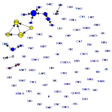
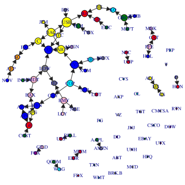
2000-2013	2007-2008

Figure 1: Graphs of estimated LVDN for the S&P100 idiosyncratic volatilities.

The LVDNs in Figure 1 are estimated in two steps. First, we obtain what we call the idiosyncratic components of volatilities by removing from the data the pervasive influence of global volatility shocks, to which we refer as common shocks or, given the present financial context, as market shocks. This is done by applying the general dynamic factor methodology recently proposed by Forni et al. (2015a, b) and adapted by Barigozzi and Hallin (2016) to a study of volatilities. More precisely, the factor model structure we are considering here is the Generalised Dynamic Factor model (GDFM) originally proposed by Forni et al. (2000) and Forni and Lippi (2001). In a second step, the LVDN is obtained by estimating and inverting a sparse vector autoregression (VAR) for the resulting idiosyncratic components, together with suitable identifying constraints. In particular, we consider VAR estimation based on three different methods: elastic net (Zou and Hastie, 2005), group lasso (Yuan and Lin, 2006), and adaptive lasso (Zou, 2006). We call this estimation approach “factor plus sparse VAR” approach.

This paper gives two main contributions to the existing financial literature on networks. First, we show that a combination of dynamic factor analysis and penalised regressions provides an ideal tool in the analysis of volatility and interconnectedness in large panels of financial time series. Second, we generalise to the high-dimensional setting the LVDN estimation originally proposed by Diebold and Yilmaz (2014) for a small number of series.

There are strong reasons in favour of our approach controlling for market volatility shocks—as opposed to a direct sparse VAR analysis that does not control for those shocks. The main motivation is of an economic nature; but forecasting and empirical motivations are important as well.

(1) Economic motivation. In the financial context, the pertinence of factor models is a direct consequence of the Arbitrage Pricing Theory (APT) and the related Capital Asset Pricing Model (CAPM) (Ross, 1976; Fama and French, 1993). These models allow us to disentangle and identify the main sources of variation driving large panels of financial time series: (i) a strongly pervasive component typically driven by few common shocks, or factors, affecting the whole market, and (ii) an idiosyncratic weakly connected component driven by local, or sectoral, shocks. In agreement with APT, the factor-driven, or common, component represents the non-diversifiable or systematic part of risk, while the idiosyncratic component, becomes perfectly diversifiable as the dimension of the system grows (Chamberlain and Rothschild, 1983). Many studies, however, provide evidence that connectivity in the idiosyncratic component, although milder than in the common component, still may be quite non-negligible, even in large dimensional systems (see for example the empirical and theoretical results by Jovanovic, 1987; Gabaix, 2011; Acemoglu et al., 2012). This is bound to happen in highly interconnected systems as financial markets. Therefore, when an exceptionally large shock, such as bankruptcy, affects the idiosyncratic component of a particular stock, that shock, although idiosyncratic, subsequently is likely to spread, and hit, eventually, all idiosyncratic components across the system. Such events are called systemic, and diversification strategies against them might be ineffective. Studying the LVDN related to the idiosyncratic volatilities, hence after controlling for market shocks, helps identifying the systemic elements of a panel of times series, and provides the basis for an analysis of contagion mechanisms.

(2) Forecasting motivation. It has been shown (see e.g. De Mol et al., 2008) that forecasts obtained via penalised regression are highly unstable in the presence of collinearity. Thus, even though forecasting is not the main goal of this paper, removing the effect of common shocks before turning to sparse VAR estimation methods seems highly advisable.

(3) Empirical motivation. When considering partial dependencies, measured by partial spectral coherence, in the idiosyncratic component, that is after common components have been removed, hidden dependencies between and within the Financial and Energy sectors are uncovered. This finding, documented in Section 5, is the empirical justification for preferring a “factor plus sparse VAR” approach rather than a direct application of sparse VAR methods.

In Section 2, we introduce the GDFM for large panels of time series and the definition of LVDN for the idiosyncratic components, allowing for a study of different sources of interdependencies. In Section 3 we discuss estimation. In Section 4, following Barigozzi and Hallin (2016), we show how to extract from financial returns those volatility proxies which will be the object of our analysis. Section 5 presents the results for the S&P100 dataset. A detailed list of the series considered and complementary results are provided in the Web-based supporting materials.

2 Factors and networks in large panels of financial time series

We consider large panels of time series data, namely, observed finite realizations, of the form $\{Y_{it}|\,i=1,\ldots,n,\ t=1,\ldots,T\}$, of some stochastic process $\mathbf{Y}:=\{Y_{it}|\,i\in\mathbb{N},\ t\in\leavevmode\nobreak\ \!\mathbb{Z}\}$; $i$ is a cross-sectional index and $t$ stands for time. Both the cross-sectional dimension $n$ and the sample size or series length $T$ are large and, in asymptotics, we consider sequences of $n$ and $T$ values tending to infinity. The notation $\mathbf{Y}_{n}:=\{\mathbf{Y}_{nt}=(Y_{1t},Y_{2t},\ldots,Y_{nt})^{\prime}|\,t\in\mathbb{Z}\}$ in the sequel is used for the $n$-dimensional subprocess of $\mathbf{Y}$; the same notation is used for all $n$-dimensional vectors. In this section, $\mathbf{Y}_{n}$ stands for a generic panel of time series. Since our interest is to study connections and interdependencies responsible for the contagion phenomenons that might lead to financial crises, then in Sections 4 and 5, we will apply the definitions and results presented here to the case of financial volatilities.

In principle, as shown by Diebold and Yilmaz (2014), a LVDN can be estimated via classical VAR estimation. However, when dealing with high-dimensional systems, VAR estimation is badly affected by curse of dimensionality problems, and adequate estimation techniques have to be considered. The most frequent strategy, in presence of large-$n$ datasets, is based on sparsity assumptions allowing for the application of penalised regression techniques (Hsu et al., 2008; Abegaz and Wit, 2013; Nicholson et al., 2014; Basu and Michailidis, 2015; Davis et al., 2015; Kock and Callot, 2015; Barigozzi and Brownlees, 2016; Gelper et al., 2016). The presence of pervasive shocks affecting the large panels of time series considered in macro-econometrics and finance has motivated the development of another dimension reduction technique, the so-called dynamic factor methods. Various versions of those methods have become daily practice in many areas of econometrics and finance; among these the GDFM by Forni et al. (2000) and Forni and Lippi (2001) is the most general, while most other factor models considered in the time series literature (Stock and Watson, 2002; Bai and Ng, 2002; Lam and Yao, 2012; Fan et al., 2013, to quote only a few) are particular cases.

2.1 The Generalised Dynamic Factor Model

In order to introduce the dynamic factor representation for $\mathbf{Y}$, we make the following assumptions.

Assumption 1.

For all $n\in\mathbb{N}$, the vector process $\mathbf{Y}_{n}$ is second-order stationary, with mean zero and finite variances.

Assumption 2.

For all $n\in\mathbb{N}$, the spectral measure of $\mathbf{Y}_{n}$ is absolutely continuous with respect to the Lebesgue measure on $[-\pi,\pi]$, that is, $\mathbf{Y}_{n}$ admits a full-rank (for any $n$ and $\theta$) spectral density matrix $\mathit{\Sigma}_{\mathbf{Y};n}(\theta)$, $\theta\in[-\pi,\pi]$ with uniformly (in $i$, $j$, $\theta$, and $n$) bounded entries $\sigma_{{\bf Y};ij}(\theta)$.

Denote by $\lambda_{\mathbf{Y};n,1}(\theta),\ldots,\lambda_{\mathbf{Y};n,n}(\theta)$, $\theta\in[-\pi,\pi]$, the eigenvalues (in decreasing order of magnitude) of $\mathit{\Sigma}_{\mathbf{Y};n}(\theta)$; the mapping $\theta\mapsto\lambda_{\mathbf{Y};n,i}(\theta)$ is also called $\mathbf{Y}_{n}$’s $i$th dynamic eigenvalue. We say that $\mathbf{Y}$ admits a General Dynamic Factor representation with $q$ factors if for all $i$ the process $\{Y_{it}\}$ decomposes into a common component $\{X_{it}\}$ and an idiosyncratic one $\{Z_{it}\}$,

$$Y_{it}=X_{it}+Z_{it}=:\sum_{k=1}^{q}b_{ik}(L)u_{kt}+Z_{it},\quad i\in\mathbb{N},\quad t\in\mathbb{Z},$$ (1)

such that

1. the $q$-dimensional vector process of factors $\mathbf{u}:=\{\mathbf{u}_{t}=(u_{1t}\;u_{2t}\ldots u_{qt})^{\prime}|\,t\in\mathbb{Z}\}$ is orthonormal zero-mean white noise;

2. the filters $b_{ik}(L)$ are one-sided and square-summable for all $i\in\mathbb{N}$ and $k=1,\ldots,q$;

3. the $q$th dynamic eigenvalue $\lambda_{\mathbf{X};n,q}(\theta)$ of $\mathbf{X}_{n}$ diverges $\theta$-almost everywhere ($\theta$-a.e.) in the interval $[-\pi,\pi]$ as $n\to\infty$;

4. the first dynamic eigenvalue $\lambda_{\mathbf{Z};n,1}(\theta)$ of $\mathbf{Z}_{n}$ is bounded ($\theta$-a.e. in $[-\pi,\pi]$) as $n\to\infty$;

5. $Z_{k,t_{1}}$ and $u_{h,t_{2}}$ are mutually orthogonal for any $k$, $h$, $t_{1}$ and $t_{2}$;

6. $q$ is minimal with respect to (i)-(v).

For any $n$, we can write (1) in vector notation as

$$\mathbf{Y}_{nt}=\mathbf{X}_{nt}+\mathbf{Z}_{nt}=:\mathit{B}_{n}(L)\mathbf{u}_{t}+\mathbf{Z}_{nt},\quad n\in\mathbb{N},\quad t\in\mathbb{Z}.$$ (2)

This actually defines the GDFM. In this model, the common and idiosyncratic components are identified by means of the following assumption on $\mathbf{Y}_{n}$’s dynamic eigenvalues.

Assumption 3.

The $q$th eigenvalue $\lambda_{\mathbf{Y};n,q}(\theta)$ of $\mathit{\Sigma}_{\mathbf{Y};n}(\theta)$ diverges, $\theta$-a.e. in $[-\pi,\pi]$, while the $(q+1)$th one, $\lambda_{\mathbf{Y};n,q+1}(\theta)$, is $\theta$-a.e. bounded, as $n\rightarrow\infty$.

More precisely, we know from Forni et al. (2000) and Forni and Lippi (2001) that, given Assumptions 1 and 2, Assumption 3 is necessary and sufficient for the process $\mathbf{Y}$ to admit the dynamic factor representation (1). Hallin and Lippi (2014) moreover provide very weak time-domain primitive conditions under which (1), hence Assumption 3, holds for some $q<\infty$.

Finally, the idiosyncratic component $\mathbf{Z}_{n}$ always admits a Wold decomposition which, after adequate transformation, yields the vector moving average (VMA) representation

$$\mathbf{Z}_{nt}:=\mathit{D}_{n}(L)\mathbf{e}_{nt},\qquad t\in\mathbb{Z},\quad\mathbf{e}_{nt}\sim w.n.({\bf 0},{\mathit{I}}_{n}),$$ (3)

where $\mathit{D}_{n}(L)=\sum_{k=0}^{\infty}\mathit{D}_{nk}L^{k}$ is a square-summable power series in the lag operator $L$. Notice that although the magnitude of those coefficients is bounded by condition (iv) above, no sparsity assumption is made.

2.2 The Long-Run Variance Decomposition Network

In order to study the interdependencies among series, and following traditional econometric analysis, we focus on the reactions of observed variables to unobserved shocks, i.e. impulse response functions. Large panels of financial time series are affected by market shocks that are, essentially, common to all stocks and represent the non-diversifiable components of risk, and by idiosyncratic shocks that are specific to one or a few stocks in the panel. The GDFM is the ideal tool for disentangling those two sources of variation: (i) the $q$ market shocks $\mathbf{u}$ and their impulse responses $\mathit{B}_{n}(L)$, defined in (2), and (ii) the $n$ idiosyncratic shocks $\mathbf{e}_{n}$ and their impulse responses $\mathit{D}_{n}(L)$, defined in (3).

Our focus here is mainly on idiosyncratic shocks. Indeed, once we control for market effects, the study of interdependencies among different stocks is strictly related to systemic risk measures, that is, individual measures of how one given stock is likely to be affected by, and/or is likely to affect, all others.

To this end, representation (3) is what we need, as it characterises all (linear) interdependencies between the components of $\mathbf{Z}_{n}$. In particular, $\mathit{D}_{n0}$ characterises contemporaneous dependencies, while $\mathit{D}_{nk}$ for $k>0$ characterises the dynamic dependencies with lag $k$. Denote by $d_{k,ij}$ the $(i,j)$th entry of $\mathit{D}_{nk}$. Then, following Diebold and Yilmaz (2014), we can summarise all dependencies up to lag $h$ by means of the forecast error variance decomposition and, more particularly, by the ratios

$$w_{ij}^{h}:=100\left(\frac{\sum_{k=0}^{h-1}d_{k,ij}^{2}}{\sum_{\ell=1}^{n}\sum_{k=0}^{h-1}d_{k,i\ell}^{2}}\right),\quad i,j=1,\ldots,n.$$ (4)

The ratio $w_{ij}^{h}$ is the percentage of the $h$-step ahead forecast error variance of $\{Y_{it}\}$ accounted for by the innovations in $\{Y_{jt}\}$. Note that, by definition,

$$\frac{1}{100}\sum_{j=1}^{n}w_{ij}^{h}=1\;\text{ for any $i$, hence }\;\frac{1}{100}\sum_{i,j=1}^{n}w_{ij}^{h}=n.$$

The LVDN is then defined by the set of edges

$$\mathcal{E}_{\text{\tiny LVDN}}:=\Big{\{}(i,j)\in\{1\ldots n\}^{2}|\ w_{ij}^{\text{\tiny LVDN}}:=\lim_{h\to\infty}w_{ij}^{h}\neq 0\Big{\}}.$$ (5)

In practice an horizon $h$ has to be chosen to compute those weights, and the operational definition of the LVDN therefore also depends on that $h$.

Three measures of connectedness can be based on the quantities defined in (4). First, we define the from-degree of component $i$ and to-degree of component $j$ (also called in-strength of node $i$ and out-strength of node $j$) as

$$\delta^{\mbox{\tiny{From}}}_{i}:=\sum_{\begin{subarray}{c}j=1,{j\neq i}\end{subarray}}^{n}w_{ij}^{h},\quad i=1,\ldots,n\quad\text{and}\quad\delta^{\mbox{\tiny{To}}}_{j}:=\sum_{\begin{subarray}{c}i=1,{i\neq j}\end{subarray}}^{n}w_{ij}^{h},\quad j=1,\ldots,n,$$ (6)

respectively. As pointed out by Diebold and Yilmaz (2014), these two measures are closely related to two classical measures of systemic risk considered in the financial literature. The from-degree is directly related with the so-called marginal expected shortfall and expected capital shortfall (of series $i$), which measure the exposure of component $i$ to extreme events affecting all other components (see Acharya et al., 2012, for a definition of these measures). As for the to-degree, it is related to co-Value-at-Risk, which measures the effect on the whole panel of an extreme event affecting component $j$ (see Adrian and Brunnermeier, 2016, for a definition). Finally, we can define an overall measure of connectedness by summing all from-degrees (equivalently, all to-degrees):

$$\delta^{\mbox{\tiny{Tot}}}:=\frac{1}{n}\sum_{i=1}^{n}\delta^{\mbox{\tiny{From}}}_{i}=\frac{1}{n}\sum_{j=1}^{n}\delta^{\mbox{\tiny{To}}}_{j}.$$ (7)

Given the economic interpretation of these quantities, the LVDN of the idiosyncratic component $\mathbf{Z}_{n}$ seems to be an ideal tool for studying systemic risk and, for this reason, in the empirical study of Section 5, we mainly focus on the LVDN of volatilities (see also Section 4 for a motivation).

An LVDN also can be constructed for the common component $\mathbf{X}_{n}$ by using a definition analogous to (4), but based on the entries of the matrix polynomial $\mathit{B}_{n}(L)$, defined in (2). However, due to the singularity of $\mathit{B}_{n}(L)$, definition (4) in this case does not measure the proportion of the $h$-step ahead forecast error variance of variable $i$ accounted for by the innovations in variable $j$, but rather the proportion of the same forecast error variance explained by the $j$th market shock $\{u_{jt}\}$.

2.3 VAR representations

The LVDN of the idiosyncratic component $\mathbf{Z}_{n}$ is defined from the coefficients of the VMA representation (3). That representation can be estimated as an inverted sparse VAR. We accordingly make the following assumption.

Assumption 4.

The idiosyncratic component $\mathbf{Z}_{n}$ admits, for some $p$ that does not depend on $n$, the VAR($p$) representation

$$\mathit{F}_{n}(L)\mathbf{Z}_{nt}=\mathbf{v}_{nt},\quad t\in\mathbb{Z},\quad\mathbf{v}_{nt}\sim w.n.(\mathbf{0},\mathit{C}^{-1}_{n}),$$ (8)

where $\mathit{F}_{n}(L)=\sum_{k=0}^{p}\mathit{F}_{nk}L^{k}$ with $\mathit{F}_{n0}=\mathit{I}_{n}$ and $\det(\mathit{F}_{n}(z))\neq 0$ for any $z\in\mathbb{C}$ such that $|z|\leq 1$, and $C_{n}$ has full rank. Moreover, denoting by $f_{k,ij}$ and $c_{ij}$ the $(i,j)$th entries of $\mathit{F}_{nk}$ and $\mathit{C}_{n}$,

$$\max_{j=1\ldots n}\sum_{i=1}^{n}\mathbb{I}_{(f_{k,ij}\neq 0)} =o(n),\quad k=1,\ldots,p,\quad n\in\mathbb{N},$$ (9)

$$\max_{i=1\ldots n}\sum_{j=1}^{n}\mathbb{I}_{(f_{k,ij}\neq 0)} =o(n),\quad k=1,\ldots,p,\quad n\in\mathbb{N},$$ (10)

$$\max_{j=1\ldots n}\sum_{i=1}^{n}\mathbb{I}_{(c_{ij}\neq 0)} =o(n),\quad n\in\mathbb{N}.$$ (11)

The first part (8) of this assumption is quite mild, provided that $p$ can be chosen large enough. The second part requires some further clarification. In (9)-(10), we require the VAR coefficient matrices in (8) to have only a small number of non-zero entries. In this sense we say that the VAR representation (8) is sparse (see, for example, the definitions of sparsity in Bickel and Levina, 2008; Cai and Liu, 2011). That assumption is needed for the consistent estimation of (8) in the large-$n$ setting, and it is justified by the idea that in a GDFM, once we control for common shocks, most interdependencies among the elements of $\mathbf{Z}_{n}$ are quite weak (since the corresponding dynamic eigenvalues are bounded as $n\to\infty$). However, note that, while a sparse VAR is related to conditional second moments, the GDFM assumptions on the idiosyncratic component are based on unconditional second moments. For this reason, the GDFM assumptions do not imply a sparse VAR representation for $\mathbf{Z}_{n}$, and (9)-(10) are needed. Finally, for convenience, we parametrise the covariance matrix of the VAR innovations by means of its inverse $\mathit{C}_{n}$ and in (11) we require this matrix to be sparse too, in accordance with the idea of a sparse global conditional dependence structure of idiosyncratic components.

As a by-product, a Long-Run Granger Causality Network (LGCN) can be defined by the set of edges

$$\mathcal{E}_{\text{\tiny LGCN}}:=\Big{\{}(i,j)\in\{1\ldots n\}^{2}|\ w_{ij}^{\text{\tiny LGCN}}:=\sum_{k=0}^{p}f_{k,ij}\neq 0\Big{\}}.$$ (12)

This network captures the leading/lagging conditional dependencies of a given panel of time series. Such graphical representations of VAR dependencies were initially proposed by Dahlhaus and Eichler (2003) and Eichler (2007), and extend to a time-series context the graphical models for independent data considered by Dempster (1972), Meinshausen and Bühlmann (2006), Friedman et al. (2008), and Peng et al. (2009), to quote only a few.

Two comments are in order here. A network is said to be sparse if its weight matrix has many zero entries. First, notice that, under Assumption 4, the LGCN is likely to be sparse. On the other hand, the GDFM assumptions do not guarantee sparsity of the LVDN but only some weaker restrictions on the magnitude of its entries, as dictated by the boundedness of the eigenvalues of $\mathbf{Z}_{n}$’s spectral density matrix. Second, the economic interpretation of the LGCN is not as straightforward as that of the LVDN, and the LGCN therefore is of lesser interest for the analysis of financial systems: mainly, it will be a convenient tool in the derivation of the LVDN. This is in line with traditional macroeconomic analysis where impulse response functions, i.e. VMA coefficients, rather than VAR ones, are the object of interest for policy makers.

As for the common component $\mathbf{X}_{n}$, Forni et al. (2015a) show that it admits the singular VAR representation

$$\mathit{A}_{n}(L)\mathbf{X}_{nt}=\mathit{H}_{n}\mathbf{u}_{t},\quad t\in\mathbb{Z},\quad\mathbf{u}_{t}\sim w.n.(\mathbf{0},\mathit{I}_{q}).$$ (13)

Assuming, without loss of generality, that $n=m(q+1)$ for some integer $m$, the VAR operator $\mathit{A}_{n}(L)$ in (13) is block-diagonal, with $(q+1)\times(q+1)$-dimensional diagonal blocks of the form $\mathit{A}^{(i)}(L)=\sum_{k=0}^{p_{i}}\mathit{A}_{k}^{(i)}L^{k}$ such that, for any $i=1,\ldots,m$, $\mathit{A}_{0}^{(i)}=\mathit{I}_{n}$ and $\det(\mathit{A}^{(i)}(z))\neq 0$ for any $z\in\mathbb{C}$ such that $|z|\leq 1$. Moreover, $\mathit{H}_{n}$ is a full-rank $n\times q$ matrix, and $\mathbf{u}$ is the $q$-dimensional process of common shocks defined in (2).

2.4 Identification

Starting from $\mathbf{Z}_{n}$’s VAR representation (8) and comparing it with (3), we have

$$\mathit{D}_{n}(L)=(\mathit{F}_{n}(L))^{-1}\mathit{R}_{n},$$ (14)

where the full-rank matrix $\mathit{R}_{n}$ is making the shocks $\mathit{R}_{n}^{-1}\mathbf{v}_{n}=:\mathbf{e}_{n}$ orthonormal (such matrices under Assumption 4 exist). In other words, the LVDN is obtained from the inversion of the VAR in (8) by selecting a suitable transformation $\mathit{R}_{n}$ meeting the required identification constraints. The simplest choice for $\mathit{R}_{n}$ follows from a Choleski decomposition of the covariance $\mathit{C}_{n}^{-1}$ of the shocks (see Sims, 1980)—namely, selecting $\mathit{R}_{n}$ as the lower triangular matrix such that $\mathit{C}_{n}^{-1}=\mathit{R}_{n}\mathit{R}_{n}^{\prime}$. Such a choice is appealing, as it is purely data-driven, but it depends on the ordering of the variables or, equivalently, on the ordering of the components of the shocks vector $\mathbf{v}_{n}$.

Many orderings are possible, and the one we propose is based on $\mathbf{v}_{n}$’s partial correlation structure. More precisely, assuming $\mathit{C}_{n}$ to have full rank, the partial correlation between $\{v_{it}\}$ and $\{v_{jt}\}$ is

$$\rho^{ij}:=\frac{-c_{ij}}{\sqrt{c_{ii}c_{jj}}},\qquad i,j=1,\ldots,n$$ (15)

where $c_{ij}$ is the $(i,j)$th entry of $\mathit{C}_{n}$. Associated with this concept of partial correlation is the Partial Correlation Network (PCN), with edges

$$\mathcal{E}_{\text{\tiny PCN}}:=\{(i,j)\in\{1\ldots n\}^{2}|\ w_{ij}^{\text{\tiny PCN}}:=\rho^{ij}\neq 0\},$$ (16)

which, by Assumption 4, is a sparse network. The PCN can be studied by means of the $n$ linear regressions

$$v_{it}=\sum_{j=1,j\neq i}^{n}\beta_{ij}v_{jt}+\nu_{it},\quad t\in\mathbb{Z},\quad\nu_{it}\sim w.n.(0,\sigma^{2}_{i}),\quad i=1,\ldots n.$$ (17)

Indeed, it can be shown that $\beta_{ij}=\rho^{ij}\sqrt{\sigma_{i}^{2}/\sigma_{j}^{2}}$ (see, for example, Lemma 1 in Peng et al., 2009), so that $(i,j)\in\mathcal{E}_{\text{\tiny PCN}}$ if and only if $\beta_{ij}\neq 0$. Thus, the inverse covariance matrix $\mathit{C}_{n}$ of the VAR shocks is directly related to the partial correlation matrix of the VAR innovations, and this matrix in turn can be seen as the PCN weight matrix. We then order the shocks by decreasing order of eigenvector centrality (as in Bonacich, 1987) in that PCN, the most central component receiving label one, etc.

The centrality measure considered defines each node’s centrality as the sum of the centrality values of its neighbouring nodes. It is easily seen that the mathematical translation of this idea leads to an eigenvector-related concept of centrality. That concept of eigenvector centrality differs from that of degree centrality (the number of neighbours of a given node); indeed, a node receiving many links does not necessarily have high eigenvector centrality, while, a node with high eigenvector centrality is not necessarily highly linked (it might have few but important linkers).

It has to be noticed that usually eigenvector centrality is defined for networks in which the sign of the weight associated to a given edge is not taken into account, so negative and positive partial correlations have the same importance. However, based on the idea that contagion is more likely between nodes which are linked through positive weights rather than negative ones, we can also consider eigenvector centrality for a signed network, thus preserving the information about weights’ signs. Both approaches are considered in the empirical analysis that follows.

This identification strategy seems well suited to the study of financial contagion. Indeed, in an impulse response exercise, we study the propagation of shocks through the system starting from lag zero up to a given lag $h>0$. Thus, a given order of shocks defines which component we choose to hit first. By ordering nodes according the their centrality in the PCN of VAR residuals, we are considering the case in which the most contemporaneously interconnected node is firstly affected by an unexpected shock, and then, by means of the subsequent impulse response analysis, we study the propagation of such shock through the whole system. The corresponding row of the LVDN adjacency matrix gives a summary, in terms of explained variance, of the effect of this propagation mechanism after $h$ lags.

Finally, it is worth mentioning a few other possible methods for identifying the shocks in the LVDN. One could rank the series based on endogenous characteristics of the firms considered, such as market capitalisation. Another data-driven approach is taken in Swanson and Granger (1997), who propose to test the over-identifying restrictions implied by orthogonal shocks. That approach is closely related to ours as those restrictions involve partial correlations of the shocks; however as the dimension $n$ of the problem increases, the related computational problems rapidly become non-tractable. Diebold and Yilmaz (2014) adopt generalised variance decompositions, a very popular method originally proposed by Koop et al. (1996). This approach, however, is only valid if the shocks have a Gaussian distribution, an assumption which is unlikely to hold true for the S&P100 dataset.

Turning to the common component $\mathbf{X}_{n}$, its LVDN is obtained by inverting the VAR representation (13). Namely, there exists a $q\times q$ invertible matrix $\mathit{K}$ such that

$$\mathit{B}_{n}(L)=(\mathit{A}_{n}(L))^{-1}\mathit{H}_{n}\mathit{K}.$$ (18)

Here $\mathit{K}$ is required in order to identify the orthonormal market shocks $\mathbf{u}$. However, if $q=1$ as in the empirical analysis of Section 5, the choice of $\mathit{K}$ reduces to that of a sign and a scale.

In the next sections, we first discuss the estimation of GDFMs and LVDNs under the general definition of this section, and then adapt to the particular case of unobserved volatilities.

3 Estimation

In this section we review estimation of (14) and (18). The numbers of factors throughout are determined via the information criterion proposed by Hallin and Liška (2007) and based on the behaviour of dynamic eigenvalues as the panel size grows from 1 to $n$. In this section we consider a generic observed panel $\{Y_{it}|\ i=1,\ldots,n,\ t=1,\ldots,T\}$ of time series, with sample size $T$ (in the next section these would be either returns or volatilities). Hereafter, we use the superscript $T$ to denote estimated quantities.

3.1 GDFM estimation

First we recover the common component using its autoregressive representation (13). For a given number of factors $q$, the method, described in detail by Forni et al. (2015a, b), is based on the following steps.

1. Estimate the spectral density matrix of $\mathbf{Y}_{n}$, denoted as $\mathit{\Sigma}_{\mathbf{Y};n}^{T}(\theta)$, for example using the smoothed periodogram estimator.

2. Use the $q$ largest dynamic principal components of $\mathit{\Sigma}_{\mathbf{Y};n}^{T}(\theta)$ to extract the spectral density matrix of $\mathbf{X}_{n}$, denoted as $\mathit{\Sigma}_{\mathbf{X};n}^{T}(\theta)$ (see Brillinger, 1981).

3. Compute the autocovariances of $\mathbf{X}_{n}$ by inverse Fourier transform of $\mathit{\Sigma}_{\mathbf{X};n}^{T}(\theta)$ and use these to compute the Yule-Walker estimator of the VAR filters $\mathit{A}_{n}^{T}(L)$; denote by $\bm{\epsilon}_{n}^{T}:=\{\epsilon_{it}^{T}|\ i=1,\ldots,n,\ t=1,\ldots,T\}$ the corresponding residuals.

4. From the sample covariance of $\bm{\epsilon}_{n}^{T}$, compute the eigenvectors corresponding to its $q$ largest eigenvalues, these are the columns of the estimator $\mathit{H}_{n}^{T}$; then, by projecting $\bm{\epsilon}_{n}^{T}$ onto the space spanned by the columns of $\mathit{H}_{n}^{T}$, obtain the $q$-dimensional vector $\{\mathbf{u}_{t}^{T}|\ t=1,\ldots,T\}$.

5. The estimated LVDN of the common component is given by $(\mathit{A}_{n}^{T}(L))^{-1}\mathit{H}_{n}^{T}\mathit{K}$, where $\mathit{K}$ is a generic $q\times q$ invertible matrix such that $\mathit{H}_{n}^{T}\mathit{K}$ consistently estimates $\mathit{H}_{n}$.

6. The estimated common and idiosyncratic components are respectively given by

   $$\mathbf{X}_{nt}^{T}=(\mathit{A}_{n}^{T}(L))^{-1}\mathit{H}_{n}^{T}\mathbf{u}_{t}^{T}\quad\text{and}\quad\mathbf{Z}_{nt}^{T}=\mathbf{Y}_{nt}-\mathbf{X}_{nt}^{T},\quad t=1,\ldots,T.$$

Details on each step and asymptotic properties of the estimators are given in Forni et al. (2015b). In particular, the parameters of the model are estimated consistently as $n$ and $T$ tend to infinity, at $O_{P}(\max({n^{-1/2},T^{-1/2}}))$ rate.

3.2 Sparse VAR estimation

Once we have an estimator of the $n$ idiosyncratic components, we estimate the VAR($p$) representation (8) by minimising the penalised quadratic loss

$$\mathcal{L}_{T}=\sum_{t=1}^{T}\bigg{(}Z_{it}^{T}-\sum_{k=1}^{p}\mathbf{f}_{k,i}^{\prime}\mathbf{Z}_{nt-k}^{T}\bigg{)}^{2}+\mathcal{P}(\mathbf{f}_{1,i}\ldots,\mathbf{f}_{p,i}),\quad i=1,\ldots,n,$$ (19)

where $\mathbf{f}_{k,i}^{\prime}$ is the $i$-th row of $\mathit{F}_{kn}$ and $\mathcal{P}(\cdot)$ is some given penalty which depends on the chosen estimation method. In particular, we consider three alternative strategies.

1. Elastic net, as defined by Zou and Hastie (2005), where the penalty is a weighted average of ridge and lasso penalties:

   $$\mathcal{P}^{EN}(\mathbf{f}_{1,i}\ldots,\mathbf{f}_{p,i})=\lambda\|(\mathbf{f}_{1,i}^{\prime}\ldots\mathbf{f}_{p,i}^{\prime})^{\prime}\|_{1}+(1-\lambda)\|(\mathbf{f}_{1,i}^{\prime}\ldots\mathbf{f}_{p,i}^{\prime})^{\prime}\|_{2}^{2}.$$

2. Adaptive lasso, as defined by Zou (2006), where the penalty is a lasso one but conditioned on a pre-estimators $\widetilde{\mathbf{f}}_{k,i}$ of the parameters (typically given by ridge or least squares estimators)

   $$\mathcal{P}^{AL}(\mathbf{f}_{1,i}\ldots,\mathbf{f}_{p,i})=\lambda\;\frac{\|(\mathbf{f}_{1,i}^{\prime}\ldots\mathbf{f}_{p,i}^{\prime})^{\prime}\|_{1}}{\|(\widetilde{\mathbf{f}}_{1,i}^{\prime}\ldots\widetilde{\mathbf{f}}_{p,i}^{\prime})^{\prime}\|_{1}}.$$

3. Group lasso, as defined by Yuan and Lin (2006), where the explanatory variables are grouped before penalising, thus in a VAR context the groups are given by the lags of each variable, thus there are $n$ groups, each of $p$ elements, and we have

   $$\mathcal{P}^{GL}(\mathbf{f}_{1,i}\ldots,\mathbf{f}_{p,i})=\lambda\sqrt{p}\sum_{j=1}^{n}\|(f_{1,ij}\ldots f_{p,ij})^{\prime}\|_{2}.$$

The penalisation constant $\lambda$, in all three methods, and the maximum VAR lag $p$, are determined by minimising, over a grid of possible values, a BIC-type criterion.

Elastic net and adaptive lasso are particularly useful in a time series context since they are known to stabilise a simple lasso estimator which might suffer on instability due to serial dependence in the data. To the best of our knowledge, elastic net so far has not been considered in the estimation of high-dimensional VARs, while adaptive lasso has been used by Kock and Callot (2015) and Barigozzi and Brownlees (2016), among others. On the other hand, group lasso in principle is likely to make the LGCN more sparse than the other two methods, and has been used, for VAR estimation, by Nicholson et al. (2014) and Gelper et al. (2016). Other possible penalised VAR estimators, which we do not consider here, include the simple lasso and smoothly clipped absolute deviation (SCAD) (see, for example, Hsu et al., 2008 and Abegaz and Wit, 2013). The consistency of all those methods is proved in the papers referenced when both $n$ and $T$ tend to infinity, under a variety of technical assumptions which we do not report here.

3.3 Identification of the LVDN

Once an estimator of the VAR coefficients is obtained, we can estimate, in a last step, the PCN of the VAR residuals, as defined in (16), which in turn can be used for LVDN identification. This again can be performed by means of several regularisation methods. Here we chose the approach proposed by Peng et al. (2009), where we refer to for technical details. More precisely, the weights of the PCN are obtained by estimating the regressions in (17) via traditional lasso (Tibshirani, 1996) in order to ensure sparsity as required by Assumption 4. Alternatively, the PCN of the residuals can be estimated jointly with the LGCN as originally proposed by Rothman et al. (2010) for cross-sectional regressions and, in a time series context, by Abegaz and Wit (2013), Gelper et al. (2016) or (with adaptive lasso penalty) Barigozzi and Brownlees (2016). Once we have estimated the PCN of VAR residuals, we can order them according to their centrality in the network. We then estimate the matrix $\mathit{R}_{n}^{T}$, needed for identification, as the Choleski factor of the sample covariance matrix of the ordered residuals. Finally, from $\mathit{R}_{n}^{T}$ and the estimated VAR operators $\mathit{F}_{n}^{T}(L)$, we compute the VMA operator $\mathit{D}_{n}^{T}(L)=(\mathit{F}_{n}^{T}(L))^{-1}\mathit{R}_{n}^{T}$. The estimated LVDNs weights, denoted as $w_{ij}^{hT}$, readily follow from (4).

It has to be noted that, while by estimating a sparse VAR the LGCN by construction is sparse, this is not the case for the LVDN which, being derived from the inverse of a sparse VAR, does not necessarily have to be sparse. In other words, the assumption of sparsity of VAR coefficients is made for the purpose of dealing with the curse of dimensionality, and does not entail sparsity of the corresponding LVDN. The matrix $\mathit{W}^{hT}$ with entries $w_{ij}^{hT}$ (the LVDN adjacency matrix) is therefore not necessarily sparse. Nevertheless, since most of its entries are quite small, considering a sparse thresholded version $\mathit{W}^{hT}_{\tau}$ with threshold $\tau>0$ is very natural. Here, we chose the threshold $\tau$ minimising the sum $\|(\mathit{W}^{hT}_{\tau}\mathit{W}^{hT^{\prime}}_{\tau})^{-1/2}(\mathit{W}^{hT}_{\tau}\mathit{W}^{hT^{\prime}}_{\tau})(\mathit{W}^{hT}_{\tau}\mathit{W}^{hT^{\prime}}_{\tau})^{-1/2}-\mathit{I}_{n}\|_{2}$ of squared errors (see for example Fan et al., 2013, for a similar approach, although in a different context).

4 Network analysis of financial volatilities

The available datasets, in the study of interdependencies of financial institutions, in general, are (large) panels of stock returns. If our interest is in the systematic, i.e. market-driven, and systemic components of risk, then volatilities are what we need, not returns. Financial crises typically are characterised by unusually high levels of volatility generated by some major systemic events as the bankruptcy of some major institutions. Analysing interdependencies in volatility panels is the first step to a study of financial contagion (see Diebold and Yilmaz, 2014, for a thorough discussion).

Volatilities unfortunately are unobserved, and therefore must be estimated from the panels of returns. Many volatility proxies can be constructed from the series of returns as, for example, the adjusted log-range (Parkinson, 1980) from daily returns, or log-realised volatilities (Andersen et al., 2003) based on intra-daily returns. Those proxies are generally treated as observed quantities, and nothing is said about the associated estimation error. On the other hand, volatilities can also be estimated from conditionally heteroschedastic models for financial returns such as multivariate GARCH models (see, for instance, the survey by Bauwens et al., 2006). Those are however parametric models which, due to the curse of dimensionality problem, cannot be handled in the present large-$n$ setting. We therefore follow the approach in Barigozzi and Hallin (2016) in adopting a global point of view, with a joint analysis of returns and volatilities in a high-dimensional setting. That analysis is based on a two-step dynamic factor procedure: a first GDFM procedure, applied to the panel of returns, is extracting a (double) panel of volatility proxies, which, in a second step, is analysed via a second GDFM. The LVDNs we are interested in are those of the common and idiosyncratic volatility components resulting from this second step.

More precisely, we consider a panel $\bm{r}_{n}:=\{\bm{r}_{nt}=(r_{1t}\;r_{2t}\ldots r_{nt})^{\prime}|\,t\in\mathbb{Z}\}$ of $n$ stock returns (such as the constituents of the S&P100 index). We assume that $\bm{r}_{n}$ satisfies Assumptions 1-3, i.e., admits the GDFM decomposition

$$\bm{r}_{nt}=\bm{\chi}_{nt}+\bm{\xi}_{nt},\quad t\in\mathbb{Z},$$ (20)

where $\bm{\chi}_{n}$ is driven by $q$ common shocks and $\bm{\xi}_{n}$ is idiosyncratic—call them level-common and level-idiosyncratic components, respectively.

When applied to the real data in Section 5, the Hallin and Liška (2007) criterion very clearly yields $q=1$, that is, a unique level-common shock. Thus the level-common component $\bm{\chi}_{n}$ admits (see (13)) the autoregressive representation

$$\mathcal{A}_{n}(L)\bm{\chi}_{nt}=:\bm{\eta}_{nt}=:(\eta_{1t},\ldots,\eta_{nt})^{\prime},\quad t\in\mathbb{Z},$$ (21)

where $\mathcal{A}_{n}(L)$ is a one-sided square-summable stable block-diagonal autoregressive filter with blocks of size $2\times 2$, and $\bm{\eta}_{n}$ is an $n$-dimensional white noise process with a singular covariance matrix of rank one.

We then assume that Assumption 4 holds for the level-idiosyncratic component $\bm{\xi}_{n}$, which thus admits the sparse VAR representation

$$\mathcal{F}_{n}(L)\bm{\xi}_{nt}=\bm{v}_{nt}=:(v_{1t},\ldots,v_{nt})^{\prime},\quad t\in\mathbb{Z}$$ (22)

where $\bm{v}_{n}$ is an $n$-dimensional white noise process and $\mathcal{F}_{n}(L)$ is a one-sided stable VAR filter with sparse coefficients, the rows of which have a finite number of non-zero terms. Estimators of $\bm{\eta}_{n}$ and $\bm{v}_{n}$ are obtained by applying the methodology described in the previous section.

Turning to volatilities, define two panels of volatility proxies,

$$\bm{\sigma}_{nt}:=\log(\bm{\eta}_{nt}^{2})\quad\text{ and }\quad\bm{\omega}_{nt}:=\log(\bm{v}_{nt}^{2}),\quad t\in\mathbb{Z},$$ (23)

with $\log(\bm{\eta}_{nt}^{2}):=(\log\eta_{1t}^{2},\ldots,\log\eta_{nt}^{2})^{\prime}$ and $\log(\bm{v}_{nt}^{2}):=(\log v_{1t}^{2},\ldots,\log v_{nt}^{2})^{\prime}$. After due centring, we assume that those two panels of volatility proxies in turn satisfy Assumptions 1-3, and hence admit the GDFM decompositions

$$\mathring{\bm{\sigma}}_{nt}:=\bm{\sigma}_{nt}-\mathrm{E}[\bm{\sigma}_{n}] =\bm{\chi}_{\sigma,nt}+\bm{\xi}_{\sigma,nt},\quad t\in\mathbb{Z},$$ (24)

$$\mathring{\bm{\omega}}_{nt}:=\bm{\omega}_{nt}-\mathrm{E}[\bm{\omega}_{n}] =\bm{\chi}_{\omega,nt}+\bm{\xi}_{\omega,nt},\quad t\in\mathbb{Z},$$ (25)

where $\bm{\chi}_{\sigma,n}$ and $\bm{\chi}_{\omega,n}$ are driven by $q_{\sigma}$ and $q_{\omega}$ common shocks, respectively, and $\bm{\xi}_{\sigma,n}$ and $\bm{\xi}_{\omega,n}$ are idiosyncratic—call them the volatility common and idiosyncratic components, respectively.

Note that traditional factor models for volatilities, derived from factor models of returns, are assuming that $\mathring{\bm{\sigma}}_{n}$ has no idiosyncratic component and, more importantly, that $\mathring{\bm{\omega}}_{n}$ has no common component. Such assumption is quite unlikely to hold, as there is no reason for market shocks only affecting the volatility $\mathring{\bm{\sigma}}_{n}$ of level-common returns. The empirical results in Barigozzi and Hallin (2016) indeed amply confirm that a non-negligible proportion of the variance of $\mathring{\bm{\omega}}_{n}$ is explained by the same market shocks also driving $\mathring{\bm{\sigma}}_{n}$.

The two volatility common components $\bm{\chi}_{\sigma,n}$ and $\bm{\chi}_{\omega,n}$ jointly define a $2n$-dimensional panel made of two blocks. These blocks might be driven by $q_{\sigma\omega}$ shocks, some of which common in both blocks, and some others common only in one of them (see Hallin and Liška, 2011, for a general theory of factor models with block structure). However, when analysing the real data in Section 5, we find that $q_{\sigma\omega}=q_{\sigma}=q_{\omega}=1$, and therefore there is evidence of a unique common shock, denoted as $\{\varepsilon_{t}\}$, driving both blocks, and thus unambiguously qualifying as the market volatility shock. The autoregressive representation of these two common components then reads as (see also (13))

$$\left(\begin{array}[]{cc}\mathit{A}_{\sigma,n}(L)&\mathit{0}_{n}\\ \mathit{0}_{n}&\mathit{A}_{\omega,n}(L)\end{array}\right)\left(\begin{array}[]{c}\bm{\chi}_{\sigma,n}\\ \bm{\chi}_{\omega,n}\end{array}\right)=\left(\begin{array}[]{c}\mathit{H}_{\sigma,n}\\ \mathit{H}_{\omega,n}\end{array}\right)\varepsilon_{t},\quad t\in\mathbb{Z},\quad\varepsilon_{t}\sim w.n.(0,1),$$ (32)

where $\mathit{A}_{\sigma,n}(L)$ and $\mathit{A}_{\omega,n}(L)$ are one-sided square-summable block-diagonal stable filters with blocks of size $2\times 2$, and $\mathit{H}_{\sigma,n}$ and $\mathit{H}_{\omega,n}$ are $n$-dimensional column vectors. All parameters in (32) can be estimated as described in Section 3.1.

The singular LVDNs for the common components of volatilities thus can be built from the VMA filters (see (18))

$$\mathit{B}_{\sigma,n}(L):=(\mathit{A}_{\sigma,n}(L))^{-1}\mathit{H}_{\sigma,n}K_{\sigma}\quad\text{and}\quad\mathit{B}_{\omega,n}(L):=(\mathit{A}_{\omega,n}(L))^{-1}\mathit{H}_{\omega,n}K_{\omega},$$ (33)

where $K_{\sigma}$ and $K_{\omega}$ in this case are just scalars needed to identify the scale and sign of the market shocks. For a given horizon $h$, the LVDN weights defined in (4) provide the percentages of $h$-step ahead forecast error variance of series $i$ accounted for by the common market shock.

For the two volatility idiosyncratic components $\bm{\xi}_{\sigma,n}$ and $\bm{\xi}_{\omega,n}$, we assume that Assumption 4 holds, yielding the sparse VAR representations

$$\mathit{F}_{\sigma,n}(L)\bm{\xi}_{\sigma,n} =\bm{\nu}_{\sigma,nt},\quad t\in\mathbb{Z},\quad\bm{\nu}_{\sigma,nt}\sim w.n.(\mathbf{0},\mathit{C}_{\sigma,n}^{-1}),$$ (34)

$$\mathit{F}_{\omega,n}(L)\bm{\xi}_{\omega,n} =\bm{\nu}_{\omega,nt},\quad t\in\mathbb{Z},\quad\bm{\nu}_{\omega,nt}\sim w.n.(\mathbf{0},\mathit{C}_{\omega,n}^{-1}),$$ (35)

where $\mathit{F}_{\sigma,n}(L)$ and $\mathit{F}_{\omega,n}(L)$ are one-sided stable filters with sparse coefficients, the rows of which have a finite number of non-zero terms. All parameters in (34) and (35) can be estimated as described in Section 3.2.

Inverting those autoregressive representations, we obtain the VMA filters (see also (14))

$$\mathit{D}_{\sigma,n}(L):=(\mathit{F}_{\sigma,n}(L))^{-1}\mathit{R}_{\sigma,n}\quad\text{and}\quad\mathit{D}_{\omega,n}(L):=(\mathit{F}_{\omega,n}(L))^{-1}\mathit{R}_{\omega,n}.$$ (36)

Here, $\mathit{R}_{\sigma,n}$ and $\mathit{R}_{\omega,n}$ are $n\times n$ invertible matrices such that $\mathit{R}_{\sigma,n}^{-1}\bm{\nu}_{\sigma,n}$ and $\mathit{R}_{\omega,n}^{-1}\bm{\nu}_{\omega,n}$ are orthonormal. As explained in Section 2, we choose those matrices to be the Choleski factors of the covariances of the VAR shocks $\bm{\nu}_{\sigma,n}$ and $\bm{\nu}_{\omega,n}$, ordered according to their centrality in the PCN induced by $\mathit{C}_{\sigma,n}$ and $\mathit{C}_{\omega,n}$ (see also (15)-(17)). From (36), and for a given horizon $h$, the LVDN weights computed from (4) then provide the shares of $h$-step ahead forecast error variance for the idiosyncratic volatility of series $i$ accounted for by innovations in the idiosyncratic volatility of series $j$. As already explained in Section 3.3, most of those weights are quite small, and naturally can be thresholded, yielding a sparse network.

5 The network of S&P100 volatilities

In this section, we consider the panel of stocks used in the construction of the S&P100 index and, based on the daily adjusted closing prices $\{p_{it}|\ i=1,\ldots,n,\ t=1,\ldots,T\}$, we compute the panel of percentage daily log-returns

$$r_{it}:=100\log\left({p_{it}/p_{it-1}}\right),\quad i=1,\ldots,n,\quad t=1,\ldots,T,$$

which are our observed “levels” or “returns”. The observation period is $T=3457$ days, from 3rd January 2000 to 30th September 2013 and, since not all 100 constituents of the index were traded during the observation period, we end up with a panel of $n=90$ time series. A detailed list of the series considered is provided in the Web-based supporting materials. All results in this section are reported for the whole period 2000-2013, and for the period 2007-2008 corresponding to the Great Financial Crisis. Networks are represented by heat-maps showing the entries of the corresponding adjacency matrices. In all those plots we highlight the Energy and Financial sectors which correspond to the index values 22-33 and 34-46, respectively. Moreover, all LVDNs considered report shocks’ effects over $h=20$ periods, corresponding to a one-month horizon (20 days plus the contemporaneous effects). Results for $h=5,10$ are reported in the Web-based supporting materials.

As already explained, the Hallin and Liška (2007) criterion yields $q^{T}=1$, that is, the level-common component is driven by a one-dimensional common shock. By estimating (20) and (21), we recover the estimated level-common component $\bm{\chi}_{n}^{T}$, the rank-one shocks $\bm{\eta}_{n}^{T}$, and the level-idiosyncratic component $\bm{\xi}_{n}^{T}$. The contribution of the level-common component to the total variation of returns, computed as the ratio between the sum of the (empirical) variances of the estimated level-common components ${\bm{\chi}}_{n}^{T}$ to the sum of the (empirical) variances of the observed returns, is 0.36. Turning to the level-idiosyncratic component $\bm{\xi}_{n}^{T}$, we recover an $n$-dimensional innovation vector $\bm{v}_{n}^{T}$ by fitting a sparse VAR.

The panels $\bm{\sigma}_{n}^{T}$ and $\bm{\omega}_{n}^{T}$ of level-common and level-idiosyncratic volatilities are constructed, as explained in (23), from the $\bm{\eta}_{n}^{T}$’s and $\bm{v}_{n}^{T}$’s; the centred panels $\mathring{\bm{\sigma}}_{n}^{T}$ and $\mathring{\bm{\sigma}}_{n}^{T}$ are obtained by subtracting the sample means. Applying the Hallin and Liška (2007) criterion again, we obtain $q_{\sigma}^{T}=q_{\omega}^{T}=1$ and, for the global panel, $q_{\sigma\omega}^{T}=1$. This implies a unique market shock, common to the two sub-panels. We then compute the estimators $\bm{\chi}_{\sigma,n}^{T}$ and $\bm{\xi}_{\sigma,n}^{T}$ of the two level-common volatility components of the GDFM decomposition (24), and the estimators $\bm{\chi}_{\omega,n}^{T}$ and $\bm{\xi}_{\omega,n}^{T}$ of the two level-idiosyncratic volatility components of the GDFM decomposition (25). The overall contribution of the common components (driven by the unique market shock, hence non-diversifiable) to the total variances of $\bm{\sigma}_{n}^{T}$ and $\bm{\omega}_{n}^{T}$ are $0.60$ and $0.17$ respectively.

5.1 The LVDN of volatility common components

We now turn to the LVDNs of the two common components $\bm{\chi}_{\sigma,n}^{T}$ and $\bm{\chi}_{\omega,n}^{T}$, given by (33). Since both panels are driven by the same unique common shock, the networks are identified once we impose a sign and a scale on the shocks. The sign is set in such a way that the sample correlation between the estimated market shock $\{\varepsilon^{T}_{t}\}$ and the cross-sectional average of all common components is positive. The scale is set in such a way that the following results represent the effect of one-standard-deviation market volatility shock, that is, the sequence of MA loading coefficients is divided by the standard error of the market shock. We then obtain the estimated filters $\mathit{B}_{\sigma,n}^{T}(L)$ and $\mathit{B}_{\omega,n}^{T}(L)$.

Since LVDNs in this case are singular, we do not show a graph, but rather report, in Table 1, for each panel $\bm{\chi}_{\sigma,n}^{T}$ and $\bm{\chi}_{\omega,n}^{T}$, the percentages of sectoral $20$-step ahead forecast error variance accounted for by the unique market shock. More precisely, for the ten sectors considered, the figures in Table 1 are the ratios

$$w_{\chi_{\sigma},j}^{T}:=100\left(\frac{\sum_{i=1}^{n_{j}}\sum_{k=0}^{20}(b_{\sigma,k,i}^{T})^{2}}{\sum_{i=1}^{n}\sum_{k=0}^{20}(b_{\sigma,k,i}^{T})^{2}}\right)\text{ and }w_{\chi_{\omega},j}^{T}:=100\left(\frac{\sum_{i=1}^{n_{j}}\sum_{k=0}^{20}(b_{\omega,k,i}^{T})^{2}}{\sum_{i=1}^{n}\sum_{k=0}^{20}(b_{\omega,k,i}^{T})^{2}}\right),\quad j=1,\ldots,10,$$

where $b_{\sigma,k,i}^{T}$ and $b_{\omega,k,i}^{T}$ are the $i$-th entries of $\mathit{B}_{\sigma,nk}^{T}$ and $\mathit{B}_{\omega,nk}^{T}$, respectively, and $n_{j}$ is the number of stocks in sector $j$. As the single shock obviously explains all the variance of the common component, we normalise the figures in each column so that their sum equals one hundred.

In both periods considered, the common component of level-common volatility is affected uniformly across all sectors by a market shock (the $w_{\chi_{\sigma},j}^{T}$ columns in Table 1), while the common components of level-idiosyncratic volatilities exhibit some interesting inter-sectoral differences (the $w_{\chi_{\omega},j}^{T}$ columns in Table 1). In particular, when looking at the $w_{\chi_{\omega},j}^{T}$ column, the Energy and Financial sectors are the most affected ones. The impact of a market shock during the crisis is even heavier on those two sectors. We refer to Barigozzi and Hallin (2016) for further results on the volatility of common components.

	2000-2013		2007-2008
Sector	$w_{\chi_{\sigma},j}^{T}$	$w_{\chi_{\omega},j}^{T}$	$w_{\chi_{\sigma},j}^{T}$	$w_{\chi_{\omega},j}^{T}$
Consumer Discretionary	10.10	7.63	9.91	7.73
Consumer Staples	10.38	10.70	9.83	10.45
Energy	9.86	13.35	9.83	27.04
Financial	10.12	13.66	10.61	18.19
Health Care	9.92	8.84	9.77	6.24
Industrials	9.41	7.59	9.59	6.34
Information Technology	10.01	10.00	10.11	3.76
Materials	9.92	6.77	10.05	9.53
Telecommunication Services	10.33	9.80	10.29	5.79
Utilities	9.96	11.67	10.01	4.93
Total	100	100	100	100

Table 1: Percentages of 20-step ahead forecast error variances due to the market shock.

5.2 The LVDN of the volatility idiosyncratic components

Turning to the idiosyncratic volatilities $\bm{\xi}_{\omega,n}^{T}$ and $\bm{\xi}_{\sigma,n}^{T}$, it appears that $\bm{\xi}_{\sigma,n}^{T}$ is essentially uncorrelated, both serially and cross-sectionally. Therefore, we focus only on the idiosyncratic volatility $\bm{\xi}_{\omega,n}^{T}$ of level-idiosyncratic components. Based on a BIC criterion, we estimate a sparse VAR(5) for $\bm{\xi}_{\omega,n}$. The weight associated with the $(i,j)$ edge of the LGCN of $\bm{\xi}_{\omega,nt}^{T}$ then is the $(i,j)$ entry of $\mathit{F}_{\omega,n}^{T}(1)=\sum_{k=0}^{5}\mathit{F}_{\omega,nk}^{T}$.

We define the edge density of a network with set of edges $\cal E$ as the proportion $\#({\mathcal{E}})/(n^{2}-n)$ of couples $(i,j)$ in $\cal E$. When considering the elastic net estimation approach, we obtain, for the period 2000-2013, a LGCN with edge density $53\%$ whereas, for the period 2007-2008, that density is close to $86\%$. The corresponding LGCNs are shown on Figure 2. Note that, as expected, the LGCNs are much sparser when resulting from group lasso estimation, with densities $14\%$ for the period 2000-2013, and $37\%$ for the period 2007-2008. Nevertheless, since the subsequent results on LVDNs turn out to be qualitatively similar regardless of the way we estimate the VAR, we only show here the elastic net results, deferring group and adaptive lasso results to the Web-based supporting materials.

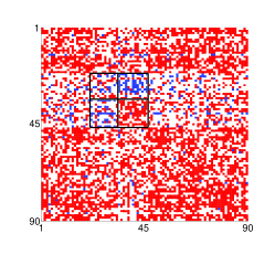
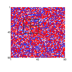
2000-2013	2007-2008

Figure 2: LGCN for $\bm{\xi}_{\omega,n}^{T}$, negative weights in blue, the positive ones in red.

As explained in the previous sections, identification of the LVDN requires some choices. The Choleski ordering is appealing, since it is data-driven, but requires an ordering of the cross-sectional items (the stocks). Here, we use an identification method based on the partial correlation of the VAR residuals $\bm{v}_{\omega,n}^{T}$. As explained in Section 2, we ordered the stocks according to the concept of eigenvector centrality for undirected networks (see Bonacich, 1987) in the estimated PCN. The resulting network is shown in Figure 3 for the two periods under study. The densities of those networks are 6% for the period 2000-2013 and 24% for the period 2007-2008. The ten most central stocks are reported in Table 2. For results using other identification methods we refer to the Web-based supporting material.

Summing up, from the estimation of the VAR model and the analysis of its residuals we see that (i) the Great Financial Crisis has considerably blown up the dynamic interdependencies between stocks, and (ii) the Energy and Financial stocks appear as the most interconnected ones, with more intra-sectoral dependencies rather than inter-sectoral.

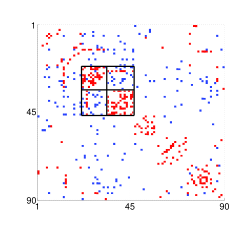
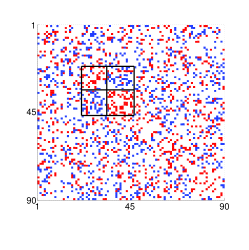
2000-2013	2007-2008

Figure 3: PCN for $\bm{\nu}_{\omega,n}^{T}$, negative weights in blue, the positive ones in red.

2000-2013	2007-2008
JPM JP Morgan Chase & Co.	BAC Bank of America Corp.
C Citigroup Inc.	USB US Bancorp
BAC Bank of America Corp.	JPM JP Morgan Chase & Co.
APA Apache Corp.	MS Morgan Stanley
WFC Wells Fargo	WFC Wells Fargo
COP Conoco Phillips	DVN Devon Energy
OXY Occidental Petroleum Corp.	GS Goldman Sachs
DVN Devon Energy	AXP American Express Inc.
SLB Schlumberger	COF Capital One Financial Corp.
MS Morgan Stanley	UNH United Health Group Inc.

Table 2: Eigenvector centrality in the PCN for $\bm{\nu}_{\omega,n}^{T}$.

percentiles	50${}^{\mbox{\tiny{th}}}$	90${}^{\mbox{\tiny{th}}}$	95${}^{\mbox{\tiny{th}}}$	97.5${}^{\mbox{\tiny{th}}}$	99${}^{\mbox{\tiny{th}}}$	max
2000-2013	0.02	0.13	0.20	0.29	0.48	4.29
2007-2008	0.17	0.71	1.00	1.28	1.76	4.53

Table 3: Selected percentiles of $\bm{\xi}_{\omega,n}^{T}$ LVDN weights.

The LVDN for $\bm{\xi}_{\omega,n}^{T}$ now can be computed on the basis of the ordering (partially) shown in Table 2. That identification defines (see (36)) the matrix $\mathit{R}_{\omega,n}^{T}$ as the Choleski factor of the sample covariance matrix of the ordered shocks. The weight of edge $(i,j)$ of the $\bm{\xi}_{\omega,n}^{T}$ LVDN is

$$w_{\xi_{\omega},ij}^{T}=100\left(\frac{\sum_{k=0}^{20}(d_{\omega,k,ij}^{T})^{2}}{\sum_{j=1}^{n}\sum_{k=0}^{20}(d_{\omega,k,ij}^{T})^{2}}\right),\quad i,j=1,\ldots,n,$$

where $d_{\omega,k,ij}^{T}$ is the $(i,j)$ entry of $\mathit{D}_{\omega,nk}^{T}$ such that $\mathit{D}_{\omega,n}^{T}(L)=\sum_{k=0}^{20}\mathit{D}^{T}_{\omega,nk}L^{k}$ as defined in (36). The resulting network is directed and weighted, but it is not sparse, meaning that in principle all its weights can be different from zero. Still, only a small proportion of edges has weights larger than one, corresponding to a proportion of variance larger than 1%. In particular, out of the total number ($n(n-1)=8010$) of possible edges, only 0.4% have weights larger than 1% over the period 2000-2013, while this number increases considerably, up to 5%, during the period 2007-2008. Selected percentiles are given in Table 3.

Figure 4 shows the $\bm{\xi}_{\omega,n}^{T}$ LVDN weights. Inspection reveals that LVDNs, although not sparse, have many entries close to zero. A thresholded version, as described in Section 3, is reported in the top row of Figure 5. The resulting plots are highly sparse and indeed the optimal value of the thresholding parameter $\tau$ is found to be 1.61 for the period 2000-2013 and 1.9 for the period 2007-2008. Plots for other values of $\tau$ are provided in the Web-based supporting materials. Given the few remaining links, this is conveniently visualised, and the corresponding networks are shown in Figure 5. Note that Financial (yellow nodes) and Energy (blue nodes) stocks are the most interconnected ones. When considering the whole sample, there are almost no inter-sectoral links; however, during the Great Financial Crisis, the degree of interconnectedness of the Financial sector with other sectors quite dramatically increases.

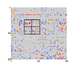
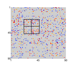
2000-2013	2007-2008

Figure 4: LVDN for $\bm{\xi}_{\omega,n}^{T}$, weights below the 95${}^{\mbox{\tiny{th}}}$ percentile in grey, between the 95${}^{\mbox{\tiny{th}}}$ and 97.5${}^{\mbox{\tiny{th}}}$ percentiles in blue, between the 97.5${}^{\mbox{\tiny{th}}}$ and 99${}^{\mbox{\tiny{th}}}$ percentiles in yellow, and above the 99${}^{\mbox{\tiny{th}}}$ percentile in red.

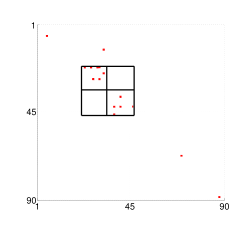
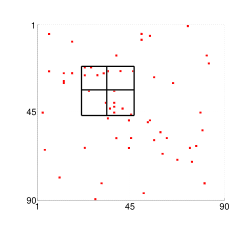
2000-2013	2007-2008

Figure 5: Thresholded LVDN for $\bm{\xi}_{\omega,n}^{T}$, non-zero weights in red.

Those findings can be quantified by computing from- and to-degrees, as defined in (6). As explained in Section 2, the from-degree measures the exposure of a given firm to shocks coming from all other firms, while the to-degree measures the effect of a shock to a given firm on all other ones. In Table 4, we show sectoral averages of from- and to-degrees when computed both for the non-sparse and thresholded LVDNs. We also report sectoral total connectedness and overall total connectedness as defined in (7). Finally, an overall measure of how systemic is an institution is given by its centrality in the network. Table 5 shows, for the two periods considered, the rankings of firms according to a measure of eigenvector centrality adapted to weighted directed networks (see Bonacich and Lloyd, 2001). For the period 2000-2013, only very few stocks are connected and qualify as central.

All results amply demonstrate that the Great Financial Crisis quite spectacularly tightened up the links between firms. In particular, when considering the thresholded LVDN version, the shocks to Financial stocks still account for almost 7% of the total idiosyncratic variance during the crisis, while shocks from other sectors explain about 5% of the Financial intra-sectoral variability (see the last two columns of Table 4). The Financial sector appears to be the most central in the network, the most vulnerable to shocks coming from all other sectors, and the most systemic in the sense that a shock to the Financial stocks is most likely to strongly affect the whole panel.

	non-thresholded				thresholded
	2000-2013		2007-2008		2000-2013		2007-2008
Sector	from	to	from	to	from	to	from	to
Consumer Discretionary	4.32	2.37	26.31	26.41	0.24	0.24	1.96	3.29
Consumer Staples	3.98	4.65	27.47	22.65	0.00	0.44	2.80	1.36
Energy	5.52	7.92	21.91	33.72	1.90	1.54	4.01	6.10
Financial	4.74	6.22	24.42	35.56	0.77	0.77	5.23	6.69
Health Care	5.00	2.51	28.06	22.36	0.00	0.00	4.27	1.83
Industrials	4.43	3.21	27.26	25.81	0.21	0.21	2.43	3.53
Information Technology	5.03	4.89	29.90	19.98	0.00	0.00	3.35	1.58
Materials	3.24	4.62	26.86	27.01	0.00	0.00	2.99	0.81
Telecommunications Services	6.50	7.26	27.44	16.52	1.91	1.91	0.00	0.00
Utilities	5.15	8.74	29.49	21.54	0.00	0.00	4.94	2.38
Total degree	4.73		26.54		0.47		3.40

Table 4: From- and To-degree sectoral averages in the $\bm{\xi}_{\omega,n}^{T}$ LVDN.

2000-2013	2007-2008
BAC Bank of America Corp.	BAC Bank of America Corp.
JPM JP Morgan Chase & Co.	AIG American International Group Inc.
C Citigroup Inc.	COF Capital One Financial Corp.
WFC Wells Fargo	USB US Bancorp
-	C Citigroup Inc.
-	WFC Wells Fargo
-	CVX Chevron
-	LOW Lowes
-	BA Boeing Co.
-	IBM International Business Machines

Table 5: Eigenvector centrality in the $\bm{\xi}_{\omega,n}^{T}$ thresholded LVDN.

A few more comments are in order in relation with the results in the Appendix. First, when comparing the results for $h=20$ with those obtained at shorter horizons ($h=5,\ 10$), we see that connectivity increases considerably with the forecast horizon, indicating that the effect of a shock keeps on propagating for a long time. This result is consistent with the fact that volatilities in financial data, although stationary, tend to have long memory (see Barigozzi and Hallin, 2016, for a detailed analysis of this aspect). Second, group lasso and elastic net VAR estimation yield qualitatively similar results. However, despite of sparser LGCNs, group lasso yields estimated LVDNs that are more tightly connected than those resulting from elastic net. This is particularly true during the crisis period when Financial and Energy stocks are the most central ones, but also the Health Care sector seems to have a decisive role.

To conclude, we provide some empirical justification of the “factor plus sparse VAR” approach adopted in this paper by comparing the conditional dependencies in the volatility panel $\bm{\omega}_{n}^{T}$ with those of its idiosyncratic component $\bm{\xi}_{\omega;n}^{T}$. To do this, we consider partial spectral coherence ($PSC$), which is the analogous of partial correlation, but in the spectral domain, and is strictly related with the coefficients of a VAR representation (see Davis et al., 2015, for a definition).

In line with the long-run spirit of the LVDN definition, and since volatilities have strong persistence, we first consider the $PSC$s at frequency $\theta=0$, thus looking at long-run conditional dependencies. Selected percentiles of the distributions of the absolute value of the PSC entries for $\bm{\omega}_{n}^{T}$ and $\bm{\xi}_{\omega;n}^{T}$ and the distribution of the absolute value of their differences are shown in Table 6. Both $PSC$s have many small (in absolute value) entries, which is consistent with our sparsity assumptions.

The two $PSC$s are shown in the first two panels of Figure 6, while in the rightmost panel we show the absolute values of their differences. Inspection of these results clearly indicates that (i) after removal of the market shock, the idiosyncratic component still contains important dependencies, and (ii) an important benefit of our “factor plus sparse VAR” approach is to uncover the hidden dependencies between and within the Financial and Energy sectors. Moreover, when repeating the same analysis at other frequencies (e.g., $\theta=\pi/2,\ \pi$), no significant difference emerges between the two $PSC$s; the benefits of our approach thus are relevant mainly in the long run.

Similar conclusions can be derived by considering spectral densities (at different frequencies) and the squared partial spectral coherence (averaged over all frequencies), a measure which is non-zero if and only if two series are uncorrelated at all leads and lags after taking into account the (linear) effects of all other series in the panel. Results are in the Web-based supporting materials.

percentiles	50${}^{\mbox{\tiny{th}}}$	90${}^{\mbox{\tiny{th}}}$	95${}^{\mbox{\tiny{th}}}$	97.5${}^{\mbox{\tiny{th}}}$	99${}^{\mbox{\tiny{th}}}$	max
$|PSC_{\bm{\omega}_{n}^{T}}(\theta=0)|$	0.06	0.16	0.18	0.22	0.25	0.35
$|PSC_{\bm{\xi}_{\omega;n}^{T}}(\theta=0)|$	0.06	0.16	0.19	0.22	0.25	0.34
$|PSC_{\bm{\omega}_{n}^{T}}(\theta=0)-PSC_{\bm{\xi}_{\omega;n}^{T}}(\theta=0)|$	0.02	0.06	0.08	0.12	0.15	0.24

Table 6: Distribution of absolute value of $PSC$s’ entries.

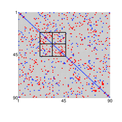
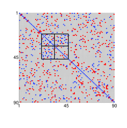
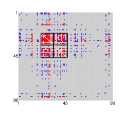
$PSC_{\bm{\omega}_{n}^{T}}(\theta=0)$	$PSC_{\bm{\xi}_{\omega;n}^{T}}(\theta=0)$	$|PSC_{\bm{\omega}_{n}^{T}}(\theta=0)-PSC_{\bm{\xi}_{\omega;n}^{T}}(\theta=0)|$

Figure 6: $PSC$s at frequency $\theta=0$. Left and middle panels: weights in absolute values below the 90${}^{\mbox{\tiny{th}}}$ percentile in grey, weights above the 90${}^{\mbox{\tiny{th}}}$ percentile in red, and below the 10${}^{\mbox{\tiny{th}}}$ percentile in blue. Right panel: weights below the 90${}^{\mbox{\tiny{th}}}$ percentile in grey, between the 90${}^{\mbox{\tiny{th}}}$ and 95${}^{\mbox{\tiny{th}}}$ percentiles in blue, and above the 95${}^{\mbox{\tiny{th}}}$ percentile in red.

6 Conclusions

In this paper, we extend the study of interconnectedness of volatility panels initiated by Diebold and Yilmaz (2014) to the high-dimensional setting where a factor structure can be assumed for the data. We determine and quantify the different sources of variation driving a panel of volatilities of S&P100 stocks over the period 2000-2013. Our analysis highlights the key role of the Financial sector, which appears to be particularly important during the Great Financial Crisis. Other sectors such as Energy, and in some cases also Health Care, seem to have an important role too. Moreover, we show that, contrary to a direct sparse VAR approach, our “factor plus sparse VAR” method can unveil crucial inter-sectoral dependencies, which can be of tantamount importance for investors’ decisions in the context of risk management.

References

- Abegaz and Wit (2013) Abegaz, F. and E. Wit (2013). Sparse time series chain graphical models for reconstructing genetic networks. Biostatistics 14, 586–599.
- Acemoglu et al. (2012) Acemoglu, D., V. M. Carvalho, A. Ozdaglar, and A. Tahbaz-Salehi (2012). The network origins of aggregate fluctuations. Econometrica 80, 1977–2016.
- Acemoglu et al. (2015) Acemoglu, D., A. Ozdaglar, and A. Tahbaz-Salehi (2015). Systemic risk and stability in financial networks. Economic Journal 125, 443–463.
- Acharya et al. (2012) Acharya, V., R. Engle, and M. Richardson (2012). Capital shortfall: a new approach to ranking and regulating systemic risks. The American Economic Review 102, 59–64.
- Adamic and Glance (2005) Adamic, L. A. and N. Glance (2005). The political blogosphere and the 2004 US election: divided they blog. In Proceedings of the 3rd international Workshop on Link Discovery, pp. 36–43. ACM.
- Adrian and Brunnermeier (2016) Adrian, T. and M. K. Brunnermeier (2016). CoVaR. The American Economic Review , forthcoming.
- Andersen et al. (2003) Andersen, T., T. Bollerslev, F. Diebold, and P. Labys (2003). Modeling and forecasting realized volatility. Econometrics 71, 579–625.
- Bai and Ng (2002) Bai, J. and S. Ng (2002). Determining the number of factors in approximate factor models. Econometrica 70, 191–221.
- Barigozzi and Brownlees (2016) Barigozzi, M. and C. Brownlees (2016). NETS: Network estimation for time series. Available at SSRN: http://ssrn.com/abstract=2249909.
- Barigozzi et al. (2010) Barigozzi, M., G. Fagiolo, and D. Garlaschelli (2010). Multinetwork of international trade: A commodity-specific analysis. Physical Review E 81, 046104.
- Barigozzi and Hallin (2016) Barigozzi, M. and M. Hallin (2016). Generalized dynamic factor models and volatilities: Recovering the market volatility shocks. The Econometrics Journal 19, 33–60.
- Basu and Michailidis (2015) Basu, S. and G. Michailidis (2015). Regularized estimation in sparse high-dimensional time series models. The Annals of Statistics 43, 1535–1567.
- Bauwens et al. (2006) Bauwens, L., S. Laurent, and J. V. K. Rombouts (2006). Multivariate GARCH models: A survey. Journal of Applied Econometrics 21, 79–109.
- Bickel and Levina (2008) Bickel, P. and E. Levina (2008). Covariance regularization by thresholding. Annals of Statistics 36, 2577–2604.
- Billio et al. (2012) Billio, M., M. Getmansky, A. Lo, and L. Pellizzon (2012). Econometric measures of connectedness and systemic risk in the finance and insurance sectors. Journal of Financial Economics 104, 535–559.
- Bonacich (1987) Bonacich, P. (1987). Power and centrality: A family of measures. American Journal of Sociology, 1170–1182.
- Bonacich and Lloyd (2001) Bonacich, P. and P. Lloyd (2001). Eigenvector-like measures of centrality for asymmetric relations. Social Networks 23, 191–201.
- Brillinger (1981) Brillinger, D. R. (1981). Time Series: Data Analysis and Theory. Holden-Day.
- Cai and Liu (2011) Cai, T. and W. Liu (2011). Adaptive thresholding for sparse covariance matrix estimation. Journal of the American Statistical Association 106, 672–684.
- Chamberlain and Rothschild (1983) Chamberlain, G. and M. Rothschild (1983). Arbitrage, factor structure, and mean–variance analysis on large asset markets. Econometrica 51, 1281–304.
- Dahlhaus and Eichler (2003) Dahlhaus, R. and M. Eichler (2003). Causality and graphical models for time series. In P. Green, N. Hjort, and S. Richardson (Eds.), Highly Structured Stochastic Systems, pp. 115–137. Oxford University Press.
- Davis et al. (2015) Davis, R. A., P. Zang, and T. Zheng (2015). Sparse vector autoregressive modeling. Journal of Computational and Graphical Statistics, to appear.
- De Mol et al. (2008) De Mol, C., D. Giannone, and L. Reichlin (2008). Forecasting using a large number of predictors: Is Bayesian shrinkage a valid alternative to principal components? Journal of Econometrics 146, 318–328.
- Dempster (1972) Dempster, A. P. (1972). Covariance selection. Biometrics 28, 157–175.
- Diebold and Yilmaz (2014) Diebold, F. and K. Yilmaz (2014). On the network topology of variance decompositions: Measuring the connectedness of financial firms. Journal of Econometrics 182, 119–134.
- Eichler (2007) Eichler, M. (2007). Granger causality and path diagrams for multivariate time series. Journal of Econometrics 137, 334–353.
- Fagiolo and Santoni (2015) Fagiolo, G. and G. Santoni (2015). Human-mobility networks, country income, and labor productivity. Network Science 3, 377–407.
- Fama and French (1993) Fama, E. F. and K. R. French (1993). Common risk factors in the returns on stocks and bonds. Journal of Financial Economics 33, 3–56.
- Fan et al. (2013) Fan, J., Y. Liao, and M. Mincheva (2013). Large covariance estimation by thresholding principal orthogonal complements. Journal of the Royal Statistical Society Series B 75, 603–680.
- Forni et al. (2000) Forni, M., M. Hallin, M. Lippi, and L. Reichlin (2000). The Generalized Dynamic Factor Model: Identification and estimation. The Review of Economics and Statistics 82, 540–554.
- Forni et al. (2015a) Forni, M., M. Hallin, M. Lippi, and P. Zaffaroni (2015a). Dynamic factor models with infinite–dimensional factor spaces: One Sided Representations. Journal of Econometrics 185, 359–371.
- Forni et al. (2015b) Forni, M., M. Hallin, M. Lippi, and P. Zaffaroni (2015b). Dynamic factor models with infinite dimensional factor space: Asymptotic analysis. EIEF working paper 16/07, einaudi institute for economics and finance, rome.
- Forni and Lippi (2001) Forni, M. and M. Lippi (2001). The Generalized Dynamic Factor Model: Representation theory. Econometric Theory 17, 1113–1141.
- Friedman et al. (2008) Friedman, J., T. Hastie, and R. Tibshirani (2008). Sparse inverse covariance estimation with the graphical lasso. Biostatistics 9, 432–441.
- Gabaix (2011) Gabaix, X. (2011). The granular origins of aggregate fluctuations. Econometrica 79, 733–772.
- Gelper et al. (2016) Gelper, S., I. Wilms, and C. Croux (2016). Identifying demand effects in a large network of product categories. Journal of Retailing 92, 25–39.
- Hallin and Lippi (2014) Hallin, M. and M. Lippi (2014). Factor models in high–dimensional time series. A time-domain approach. Stochastic Processes and their Applications 123, 2678–2695.
- Hallin and Liška (2007) Hallin, M. and R. Liška (2007). Determining the number of factors in the general dynamic factor model. Journal of the American Statistical Association 102, 603–617.
- Hallin and Liška (2011) Hallin, M. and R. Liška (2011). Dynamic factors in the presence of blocks. Journal of Econometrics 163, 29–41.
- Hautsch et al. (2014) Hautsch, N., J. Schaumburg, and M. Schienle (2014). Forecasting systemic impact in financial networks. International Journal of Forecasting 30, 781–794.
- Hautsch et al. (2015) Hautsch, N., J. Schaumburg, and M. Schienle (2015). Financial network systemic risk contributions. Review of Finance 19, 685–738.
- Hsu et al. (2008) Hsu, N.-J., H.-L. Hung, and Y.-M. Chang (2008). Subset selection for vector autoregressive processes using lasso. Computational Statistics & Data Analysis 52, 3645–3657.
- Jovanovic (1987) Jovanovic, B. (1987). Micro shocks and aggregate risk. The Quarterly Journal of Economics 102, 395–409.
- Kock and Callot (2015) Kock, A. B. and L. Callot (2015). Oracle inequalities for high dimensional vector autoregressions. Journal of Econometrics 186, 325–344.
- Kolaczyk (2009) Kolaczyk, E. D. (2009). Statistical Analysis of Network Data: Methods and Models. Springer Science & Business Media.
- Koop et al. (1996) Koop, G., M. H. Pesaran, and S. M. Potter (1996). Impulse response analysis in nonlinear multivariate models. Journal of econometrics 74, 119–147.
- Lam and Yao (2012) Lam, C. and Q. Yao (2012). Factor modeling for high-dimensional time series: inference for the number of factors. The Annals of Statistics 40, 694–726.
- Meinshausen and Bühlmann (2006) Meinshausen, N. and P. Bühlmann (2006). High-dimensional graphs and variable selection with the Lasso. The Annals of Statistics 34, 1436–1462.
- Newman (2001) Newman, M. E. (2001). The structure of scientific collaboration networks. Proceedings of the National Academy of Sciences 98, 404–409.
- Nicholson et al. (2014) Nicholson, W. B., J. Bien, and D. S. Matteson (2014). Hierarchical vector autoregression. arXiv preprint 1412.5250.
- Parkinson (1980) Parkinson, M. (1980). The extreme value method for estimating the variance of the rate of return. The Journal of Business 53, 61–65.
- Peng et al. (2009) Peng, J., P. Wang, N. Zhou, and J. Zhu (2009). Partial correlation estimation by joint sparse regression models. Journal of the American Statistical Association 104, 735–746.
- Ross (1976) Ross, S. A. (1976). The arbitrage theory of capital asset pricing. Journal of Economic Theory 13, 341–360.
- Rothman et al. (2010) Rothman, A. J., E. Levina, and J. Zhu (2010). Sparse multivariate regression with covariance estimation. Journal of Computational and Graphical Statistics 19, 947–962.
- Serrano and Boguñá (2003) Serrano, M. Á. and M. Boguñá (2003). Topology of the world trade web. Physical Review E 68, 015101.
- Sims (1980) Sims, C. A. (1980). Macroeconomics and reality. Econometrica 48, 1–48.
- Stock and Watson (2002) Stock, J. H. and M. W. Watson (2002). Forecasting using principal components from a large number of predictors. Journal of the American Statistical Association 97, 1167–1179.
- Swanson and Granger (1997) Swanson, N. R. and C. W. Granger (1997). Impulse response functions based on a causal approach to residual orthogonalization in vector autoregressions. Journal of the American Statistical Association 92, 357–367.
- Tibshirani (1996) Tibshirani, R. (1996). Regression shrinkage and selection via the lasso. Journal of the Royal Statistical Society Series B, 267–288.
- Watts and Strogatz (1998) Watts, D. J. and S. H. Strogatz (1998). Collective dynamics of “small-world” networks. Nature 393, 440–442.
- Yuan and Lin (2006) Yuan, M. and Y. Lin (2006). Model selection and estimation in regression with grouped variables. Journal of the Royal Statistical Society Series B 68, 49–67.
- Zachary (1977) Zachary, W. W. (1977). An information flow model for conflict and fission in small groups. Journal of Anthropological Research 33, 452–473.
- Zou (2006) Zou, H. (2006). The adaptive lasso and its oracle properties. Journal of the American Statistical Association 101, 1418–1429.
- Zou and Hastie (2005) Zou, H. and T. Hastie (2005). Regularization and variable selection via the elastic net. Journal of the Royal Statistical Society Series B 67, 301–320.