A Makespan Lower Bound for the Scheduling of the Tiled Cholesky Factorization based on ALAP scheduling

Abstract

Due to the advent of multicore architectures and massive parallelism, the tiled Cholesky factorization algorithm has recently received plenty of attention and is often referenced by practitioners as a case study. It is also implemented in mainstream dense linear algebra libraries. However, we note that theoretical study of the parallelism of this algorithm is currently lacking. In this paper, we present new theoretical results about the tiled Cholesky factorization in the context of a parallel homogeneous model without communication costs. We use standard flop-based weights for the tasks. For a $t$-by-$t$ matrix, we know that the critical path of the tiled Cholesky algorithm is $9t-10$ and that the weight of all tasks is $t^{3}$. In this context, we prove that no schedule with less than $0.185t^{2}$ processing units can finish in a time less than the critical path. In perspective, a naive bound gives $0.11t^{2}.$ We then give a schedule which needs less than $0.25t^{2}+0.16t+3$ processing units to complete in the time of the critical path. In perspective, a naive schedule gives $0.50t^{2}.$ In addition, given a fixed number of processing units, $p$, we give a lower bound on the execution time as follows:

$$\max(\frac{t^{3}}{p},\frac{t^{3}}{p}-3\frac{t^{2}}{p}+6\sqrt{2p}-7,9t-10).$$

The interest of the latter formula lies in the middle term. Our results stem from the observation that the tiled Cholesky factorization is much better behaved when we schedule it with an ALAP (As Late As Possible) heuristic than an ASAP (As Soon As Possible) heuristic. We also provide scheduling heuristics which match closely the lower bound on execution time. We believe that our theoretical results will help practical scheduling studies. Indeed, our results enable to better characterize the quality of a practical schedule with respect to an optimal schedule.

I Introduction

Most time-consuming tasks performed on supercomputers are linear algebra operations. With the advent of multicore architectures and massive parallelism, this results in the necessity to optimize and understand their parallel executions. Here, we consider the problem of the tiled Cholesky factorization. The algorithm divides the initial matrix into square sub-matrices, or tiles of the same size. The focus will be on large instances of the tiled Cholesky factorization, that is where the number of tiles is large, which allows asymptotical analysis. To the authors’ knowledge, no theoretical non trivial bound on the execution time of any schedule for the tiled Cholesky factorization have been found. This motivates this paper.

We note that the tiled Cholesky factorization algorithm has recently received plenty of attention. Either as an algorithm in itself [1, 2] or as a case study for task-based schedulers [3, 4, 5, 6, 7, 8]. Examples of task-based schedulers which have produced papers about the scheduling of tiled Cholesky factorization are for example DAGuE [9], KAAPI [10], QUARK [11], StarPU [12], SMPSs [13], and SuperMatrix [14]. We also note that OpenMP since 3.1 supports task-based parallelism. The tiled Cholesky factorization algorithm is also used in practice and is implemented in Dense Linear Algebra state of the art libraries, for example DPLASMA, FLAME, and PLASMA.

It is therefore of interest to better understand the parallel execution of the tiled Cholesky factorization algorithm. In this paper, we neglect communication costs between processing units. We also ignore any memory problems a real execution would encounter. Also, we assume homogeneous processing units. Also, we assume ideal flop-based weights for the execution time of the tasks. While we acknowledge that this is a very unrealistic and simplistic model, we note that any practical implementations will execute slower than this model. Therefore, this model provides lower bounds on the execution time of any parallel execution on any parallel machine. The lower bounds that we exhibit are not trivial and are relevant for practical applications.

We can relate our work to the recent work of Agullo et al. [6] where the authors provide lower bound as well. The authors consider a more complicated model (heterogeneous) and solve their problem with an LP formulation. We consider a simpler model (homogeneous) but we provide closed-form solutions. Another contribution of our paper is the ALAP schedule heuristic where tasks are scheduled from the end of the execution as opposed from the start.

We can also relate our work to the work of Cosnard, Marrakchi, Robert, and Trystram from 1988 to 1989 [15, 16, 17]. In this work, the authors have the same model and ask similar questions as ours. A minor difference is that they are studying the Gaussian elimination while we study the Cholesky factorization. The main difference is that they study the Level 1 BLAS algorithm which work on columns of the matrix. This algorithm was popular in the 1980s due to vectorization, nowadays tiled algorithms are much more relevant. Also the scheduling of the Level 1 BLAS algorithm seems to be an easier problem. In the Level 1 BLAS algorithm, the matrix is partitioned by columns. The number of created tasks is $\mathcal{O}(t^{2})$ where $t$ is the number of columns of the problem. In our case, we partition the matrix by tiles. If we have a $t$-by-$t$ tile matrix, the number of created tasks is $t^{3}$. We have tried to apply similar techniques as in the Level 1 BLAS algorithm study papers to solve the tiled problem and we have been unsuccessful. We have tried to solve the the Level 1 BLAS algorithm problem with our techniques and have obtained the same results.

A few scheduling algorithms exist for the (tiled) Cholesky factorization ; in practice, the ALAP (As Late As Possible) schedule seems to work well with the tiled Cholesky factorization. This motivates our study of this heuristic in Section III. In particular, we derive an upper bound on the number of processing units necessary to reach the critical path of the algorithm. Then, we present in Section IV some lower bounds on the execution time of any schedule using a given number of processing units by splitting the task set into two subsets. In Section V, we analyze the last bound found in Section IV, and show that it is nearly optimal by describing a schedule with efficiency close to the efficiency bound derived from it.

II Context, Definitions, Assumptions

Given a Symmetric Positive Definite (SPD) matrix $A$, the Cholesky factorization gives a (lower) triangular matrix $L$ such that $A=LL^{T}$. It is a core operation to compute the inverse of SPD matrices using the Cholesky inversion. Note that it also allows to solve systems of the form $Ax=b$ by reducing it to computing solutions of $Ly=b$, and then $L^{T}x=y$.

In order to compute such a factorization using many processing units, we divide the matrix $A$ into $t\times t$ square tiles of size $n_{b}$. This allows tile computations, and globally increases the amount of parallelism and the data locality. Algorithm 1 computes the Cholesky factorization of $A$ using these blocks.

Algorithm 1 Tiled Cholesky Factorization

  for $k=0$ to $t-1$ do

     $A_{k,k}\leftarrow POTRF(A_{k,k})$                {$C_{k}$}

     for $i=k+1$ to $t-1$ do

        $A_{i,k}\leftarrow TRSM(A_{k,k},A_{i,k})$         {$T_{i,k}$}

     end for

     for $j=k+1$ to $n-1$ do

        $A_{j,j}\leftarrow SYRK(A_{j,k},A_{j,j})$         {$S_{j,k}$}

        for $i=j+1$ to $n-1$ do

           $A{i,j}\leftarrow GEMM(A_{i,k},A_{j,k})$   {$G_{i,j,k}$}

        end for

     end for

  end for

We will rename the tasks corresponding to the POTRF as $C$ or $C_{i}$ with $1\leq i\leq t$ (as POTRF is a $n_{b}$-by-$n_{b}$ Cholesky factorization), TRSM as $T$ or $T_{i,j}$ with $1\leq j<i\leq t$, SYRK as $S$ or $S_{i,j}$ with $1\leq j<i\leq t$, and GEMM as $G$ or $G_{i,j,k}$ with $1\leq k<j<i\leq t$ to refer to the tasks in Algorithm 1.

We neglect any communication cost here. Also, tasks $C,T,S,G$ will be considered as elementary: at most one processing unit can execute such a task at a given time (no divisible load).

The dependencies between the tasks are given by:

• $C_{j}\rightarrow T_{i,j},j<i\leq t$;

• $T_{i,j}\rightarrow S_{i,j},j<i\leq t$;

• $T_{i,j}\rightarrow G_{i,k,j},j<k<i\leq t$;

• $T_{i,j}\rightarrow G_{k,i,j},j<i<k\leq t$;

• $S_{i,j}\rightarrow S_{i,j+1},j+1<i\leq t$;

• $S_{i,i-1}\rightarrow C_{i},1<i\leq t$;

• $G_{i,j,j-1}\rightarrow T_{i,j},1<j<i\leq t$;

• $G_{i,j,k}\rightarrow G_{i,j,k+1},k+1<j<i\leq t$.

Figure 1 presents the Directed Acyclic Graph (DAG) of the dependencies between the tasks of a $5\times 5$ tiled Cholesky Factorization.

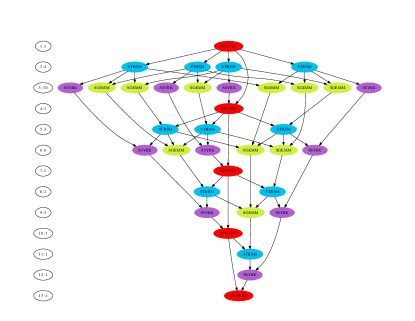
Figure 1: DAG of a $5\times 5$ Cholesky factorization

For a task $X$, $cp(X)$ will denote the critical path of task $X$, and $w(X)$ its weight.

The number of tasks of each kind is given in Table I.

TABLE I: Number of tasks

Type of task	Number of tasks
C	$t$
S	$\frac{t(t-1)}{2}$
T	$\frac{t(t-1)}{2}$
G	$\frac{t^{3}}{6}-\frac{t^{2}}{2}+\frac{t}{3}$

Moreover, we will assume that $n_{b}$ is large, so that the weights of the tasks can be those of Table II. As a result, for the rest of this study, we will consider $\frac{1}{3}n_{b}^{3}$ as time unit: executing a POTRF will take $1$ unit of time, executing a SYRK or a TRSM will take $3$ steps, and a GEMM $6$ steps.

TABLE II: Task weights for the Cholesky factorization

Type of Task	number of Flops	Weight (in $\frac{1}{3}n_{b}^{3}*$Flops)
POTRF ($C$)	$\frac{1}{3}n_{b}^{3}+\mathcal{O}(n_{b}^{2})$	1
TRSM ($T$)	$n_{b}^{3}$	3
SYRK ($S$)	$n_{b}^{3}+\mathcal{O}(n_{b}^{2})$	3
GEMM ($G$)	$2n_{b}^{3}+\mathcal{O}(n_{b}^{2})$	6

We can also count the number of tasks of each kind, and their critical path. The respective critical paths for the tasks are given in Table III, which gives the values in Table IV.

TABLE III: Critical paths of the tasks

Task	Critical Path
$C_{i}$	$C_{i}-T_{i+1,i}-G_{i+2,i+1,i}-T_{i+2,i+1}-...$
	$...-T_{t,t-1}-S_{t,t-1}-C_{t}$
$T_{i,j}$	$T_{i,j}-G_{i,j+1,j}-T_{i,j+1}-...$
	$...-T_{i,i-1}-G_{i+1,i,i-1}-T_{i+1,i}-...$
$S_{i,j}$	$S_{i,j}-S_{i,j+1}-...-S_{i,i-1}-C_{i}-...$
$G_{i,j,k}$	$G_{i,j,k}-G_{i,j,k+1}-...-G_{i,j,j-1}-T_{i,j}-...$

TABLE IV: Weight of critical paths of the tasks

Task	Weight of Critical Path
$C_{i}$	$1$ if $i=t$
	$9(t-i)-1$ otherwise
$T_{i,j}$	$9(t-j)-2$
$S_{i,j}$	$3(t-j)+1$ if $i=t$
	$9t-6i-3j-1$ otherwise
$G_{i,j,k}$	$9t-3j-6k-2$

In particular the critical path for the algorithm ($CP$) is reached for task $C_{1}$, and equals $9t-10$.

The total work ($TW$) of the Cholesky factorization, that is the sum of the weights of all tasks of the algorithm, equals $t^{3}$ (with $\frac{1}{3}n_{b}^{3}$ as the work unit).

Note that as the total work is in $\mathcal{O}(t^{3})$, and as the global critical path of the algorithm is $\mathcal{O}(t)$, a number $p=\mathcal{O}(t^{2})$ of processing units is required to achieve a makespan equal to the critical path. For that reason, our results will be presented with a number of processing units $p=\alpha t^{2}$, and with $t$ large to allow such an analysis.

III The ALAP (As Late As Possible) schedule

In this section, we analyze the ALAP schedule for the $t\times t$ tiled Cholesky factorization. This heuristic seems indeed to perform quite well. The schedule is executed as follows: the elementary tasks (POTRF, SYRK, TRSM, GEMM) are sorted according to their critical path. Then the tasks with least critical path are set to be executed last; those with least critical path among the remaining tasks set to be executed the latest possible so that the previous ones can be executed, etc. Thus, if this schedule has a makespan $\tau$ and has enough processing units, task $X$ will begin its execution at time $\tau-cp(X)$ where $cp(X)$ denotes the critical path of task $X$. Therefore, we study the distribution of the critical paths of the tasks to understand how many processing units are required to run an optimal ALAP schedule.

The section flows as follows. First we analyze the ALAP schedule to obtain the number of tasks executed at each ticks of the algorithm. The results are presented in Table V. Then we established simpler lower bounds and upper bounds to study this function. These bounds are given in Table VI and Table VII. In Figure 3, we plot the exact function and our associated lower and upper bounds for $t=60$. We note that our lower and upper bounds are assymptotically close to the function. Finally we conclude the section with an upper bound on the number of processors needed to obtain a makepsan equal to the critical path.

Figure 2 shows the execution of an ALAP schedule with sufficiently many processing units on a $8\times 8$ tiled Cholesky factorization, with every rectangle representing a task, and the time on the x-axis.

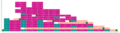
Figure 2: ALAP schedule on $8\times 8$ tiles. Dark green POTRF, light green for TRSM, salmon for SYRK, and magenta for GEMM. Time is in the x-axis. Execution time is the critical path length: $9t-10=62$. Number of required processing units for the schedule is 16.

More precisely, we want to determine, at time $\tau-K$, where $K$ denotes a critical path parameter, how many tasks are executed with an ALAP schedule with sufficiently many processing units. Note that the execution of a task $X$ starts at $\tau-cp(X)$, but ends at $\tau-cp(X)+w(X)$. Therefore, such a task $X$ should count as being executed for times $\tau-cp(X)$ to $\tau-cp(X)+w(X)-1$ (we suppose that at time $\tau-cp(X)+w(X)$, the execution of task $X$ has finished).

With that in mind, we can count the number of tasks of each kind (POTRF, SYRK, TRSM, GEMM) being executed at a time $\tau-K$.

Counting the tasks C and T is straightforward with the formulas of Table IV.

To count the tasks S, note that the S-floor of level $i$, $i<t$ defined by being the set $\left\{S_{i,j}\right\}_{j<i}$ begins at $K^{(i)}_{min}=8+9(t-i-1)=9(t-i)$ and ends at $K^{(i)}_{max}=8+9(t-i-1)+1+3(i-1)-1=9t-6i-4$, and that for any $K$ in-between, exactly $1$ task of the S-floor of level $i$ is executed. Note that the S-floor of level $i$ starts (resp. ends) before level $i-1$ starts (resp. ends) with respect to $K$. Therefore, for any $K$, there are some $i_{min}>1$ and $i_{max}<t$, such that at time $\tau-K$, exactly one task from every floor $i$, $i_{min}\leq i\leq i_{max}$ is executed; we then add the S-floor of level $t$, which starts at $K=2$ and ends at $K=3t-2$. And these are the only SYRKs being executed at that time. The expressions of $i_{min}$ and $i_{max}$ follow by noticing that $i_{max}$ (resp. $i_{min}$) corresponds to the largest $i$ such that $cp(S_{i,1})\geq K$, i.e. the S-floor of level $i_{max}$ starts before $\tau-K$ (resp. the least $i$ such that $cp(S_{i,i-1})\leq K$: the S-floor of level $i_{min}$ finishes before $\tau-K$), and using Table IV.

For the tasks G, let us fix $K$. Let $J=\left\{j|\textmd{ some }G_{i,j,k}\textmd{ is executed at time }\tau-K\right\}$. Note that $G_{i,j,k}$ is executed at time $\tau-K$ if and only if $K\leq cp(G_{i,j,k})\leq K+5$, as tasks G require 6 steps of time to be executed. The expression of the critical path of the tasks G gives that $J$ is an integer interval $\llbracket j_{min},j_{max}\rrbracket$, and that for all $j\in J$, there is a unique $k_{j}$ such that $G_{i,j,k_{j}}\textmd{ is executed at time }\tau-K$. Also, for all $j\in J$, any $G_{i,j,k_{j}}$ where $j<i\leq t$ is executed at time $\tau-K$ (a whole G-column is executed). To compute $j_{min}$ (resp. $j_{max}$), one necessary and sufficient condition is that $cp(G_{i,j_{min},k})\geq K$ for some $k$ (resp. $cp(G_{i,j_{max},k})\leq K$ for some $k$), which is equivalent to the fact that $cp(G_{i,j,j-1})\geq K$ (resp.$cp(G_{i,j,1})\leq K$).

This reasoning gives Table V where we can find the following formulas, with $M_{X,K}$ being the number of tasks of type X being executed at time $\tau-K$ in an ALAP schedule with sufficiently many processing units.

TABLE V: The heights of the ALAP schedule

$M_{X,K}$ is the number of tasks of type X being executed at time $\tau-K$ in an ALAP schedule with sufficiently many processing units. $\displaystyle M_{C,K}$ $\displaystyle=$ $\displaystyle\left\{\begin{array}[]{cl}1&\textmd{ if }K=9\ell+8,\\ 0&\textmd{ else.}\end{array}\right.$ (3) $\displaystyle M_{T,K}$ $\displaystyle=$ $\displaystyle\left\{\begin{array}[]{cl}\ell+1&\textmd{ if }9\ell+5\leq K\leq 9\ell+7\\ 0&\textmd{ else.}\end{array}\right.$ (6) $\displaystyle M_{S,K}$ $\displaystyle=$ $\displaystyle\left\{\begin{array}[]{cl}i_{max}-i_{min}+2&\textmd{if }2\leq K\leq 3t-2\\ \\ i_{max}-i_{min}+1&\textmd{otherwise}\end{array}\right.$ (10) $\displaystyle M_{G,K}$ $\displaystyle=$ $\displaystyle\sum_{j=j_{min}+1}^{j_{max}}\left(t-j\right)$ where $i_{max}=\min\left(t,\lfloor\frac{3t}{2}-\frac{K}{6}-\frac{7}{12}\rfloor\right)$ and $i_{min}=\lceil t-\frac{K}{9}\rceil$ denote the two extremal S-floors executed at time $\tau-K$, and $j_{max}=\min\left(t-1,\lfloor 3t-\frac{K}{3}-\frac{8}{3}\rfloor\right)$, $j_{min}=\lceil t-\frac{K}{9}-\frac{2}{9}\rceil$ are as defined above.

We can now divide the execution time of the ALAP schedule into three zones.

In a first zone, both $i_{max}$ and $j_{max}$ are constrained, as they cannot be greater than $t$ and $t-1$ respectively. One possible interpretation is that for a bigger instance of Cholesky factorization (with $t^{\prime}>t$), other S-floors would have been executed in this zone; in addition to the floors, other G-columns would have been executed. This zone is delimited by $K<3t+2:=K_{S}$. We will call this zone Zone 1.

In a second zone, $i_{max}$ is constrained by $t$, but $j_{max}$ is not constrained. It corresponds to $K_{S}<K\leq K_{G}:=6t-5$. We will call this zone Zone 2.

In a third zone, $i_{max}$ and $j_{max}$ are not constrained; it is the case as long as $K>K_{G}$. We will call this zone Zone 3.

Summing these formulas give the height of the ALAP schedule we look for. But because of the ceils and floors, we will not get any clear formula at the end. As a result, we focus on getting lower bounds and upper bounds on the height, by using $x\leq\lceil x\rceil<x+1$, and $x-1<\lfloor x\rfloor\leq x$. Let us note $h(t,K)$ the number of tasks being executed at time $\tau-K$ by an ALAP schedule with sufficiently many processing units. We have $h(t,K)=M_{C,K}+M_{T,K}+M_{S,K}+M_{G,K}$. That gives the formulas in Tables VI and VII.

TABLE VI: Lower bound on the height of the ALAP schedule

Zone	Lower bound on height
1	$\frac{K^{2}}{162}-\frac{5K}{162}-\frac{25}{81}$
2	$\frac{K^{2}}{162}-\frac{16K}{162}+\frac{t}{2}-\frac{289}{324}$
3	$-\frac{4K^{2}}{81}+\frac{2Kt}{3}-\frac{197K}{162}-2t^{2}+\frac{119t}{18}-\frac{587}{108}$

TABLE VII: Upper bound on the height of the ALAP schedule

Zone	Upper bound on height
1	$\frac{K^{2}}{162}+\frac{31K}{162}+\frac{155}{81}$
2	$\frac{K^{2}}{162}+\frac{2K}{81}+\frac{t}{2}+\frac{755}{324}$
3	$-\frac{4K^{2}}{81}+\frac{2Kt}{3}-\frac{107K}{162}-2t^{2}+\frac{83t}{18}+\frac{37}{108}$

In Figure 3, we plot the exact distribution of the execution of the tasks, and the upper and lower bound functions. We note that our lower and upper bounds are assymptotically close to the function. From this figure, we see that for $t=60$ tiles, we have a schedule that executes in $9t-10$ (=530) for 907 processing units. Our upper bound (which is simpler to analyze) guarantees that we need at most 913 processing units.

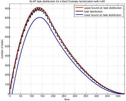
Figure 3: ALAP distribution for $t=60$ tiles. In black is the exact distribution. Red is the upper bound. Blue is the lower bound.

Note that the maximum height of the distribution (that is the minimum number of processing units required to run the ALAP schedule optimally) is reached in Zone 3, i.e. where $K>6t-5$. That phenomenon is verified experimentally. It can also be deduced from the fact that the height in the two other zones is essentially a degree 2 polynomial in $K$ with positive leading coefficient (which comes from the number of G executed); therefore by convexity the maximum height there is reached at the extremities of the zones. The result follows by observing that the height in the third zone is increasing at its beginning.

From that, we obtain the maximum height of the distribution, which gives the minimal number of processing units required to run the ALAP schedule:

$$\forall K,h(t,K)\leq\frac{1}{4}t^{2}+\frac{11}{72}t+\frac{13225}{5284}.$$

We deduce an upper bound on the number of processing units required to reach the critical path of the Cholesky factorization:

Theorem.

The ALAP schedule of a $t\times t$ tiled Cholesky factorization completes in the critical path time ($9t-10$) using less than $p=0.25t^{2}+0.16t+3$ processing units.

We note that this results is much better than what an ASAP schedule would give. The ASAP schedule of a $t\times t$ tiled Cholesky factorization completes in the critical path time ($9t-10$) critical path using $p=0.5t(t-1)$ processing units. The analysis is easy and is based on the fact that, with an ASAP schedule, after the first POTRF and the first $t-1$ TRSM, one has $0.5(t-2)(t-1)$ SYRK and GEMM tasks to execute.

IV Lower bounds

We now consider lower bounds on the makespan of the Cholesky factorization. To that purpose, we split the task set into two parts, and combine lower bounds on the execution time of both parts.

It is well known and clear that the makespan of any schedule working on a given algorithm with $p$ processing units is greater than $\max(TW/p,CP)$ (where $TW$ is the total work necessary to finish the algorithm, $CP$ its critical path). Indeed, $TW/p$ corresponds to a schedule that achieves full parallelism during its whole execution with p processing units; and no schedule can execute the algorithm faster than $CP$.

The idea here will be to combine those two bounds: let $K$ be a critical path parameter. Let $E_{2}$ be the set of tasks $X$ such that $cp(X)-w(X)\leq K$, and $E_{1}$ be its complement.

Note that in the general case, $E_{2}$ contains some tasks with critical path $\geq K$. Indeed, any task of $E_{2}$ without parents in $E_{2}$ necessarily has critical path $\geq K$ (else any of its parents would have been in $E_{2}$ too). Also, as long as $E_{1}$ and $E_{2}$ are not empty, some task in $E_{1}$ has a child in $E_{2}$ (the two sets cannot be disconnected).

Note also that all the tasks in $E_{1}$ have critical path $>K$.

Define for a set $E$ of tasks, the total weight of $E$ $w(E)=\sum_{X\in E}w(X)$ the sum of the weights of the tasks in $E$. The basic idea is that one will essentially require time $\geq w(E_{1})/p$ to execute $E_{1}$ and time $\geq K$ to execute $E_{2}$.

This results in the following claim to prove our lower bound:

Claim.

Let $K$ be a critical path parameter. Let $E_{2}$ be the set of tasks $X$ such that $cp(X)-w(X)\leq K$, and $E_{1}$ be its complement. Then the makespan of any schedule for using $p$ processing units is greater than

$$\max(CP,\frac{w(E_{1})}{p}+K)$$

Proof.

Suppose by contradiction that there exists a schedule executing the algorithm in time $\tau<\frac{TW-w(E_{1})}{p}+K$. If $\tau<K$, then the schedule cannot execute $E_{2}$ (defined above) in time $\tau$, as $E_{2}$ contains some tasks with critical path $\geq K$, which gives a contradiction. Therefore $\tau\geq K$.

Then, let us write $\tau=(\tau-K)+K$. Then $\tau-K<\frac{w(E_{1})}{p}$ by hypothesis. So after time $\tau-K$, $E_{1}$ cannot be fully executed, according to the naive bound. Therefore, there is a task from $E_{1}$ that is not fully completed at time $\tau-K$, and the remaining tasks cannot be executed in time $K-1$ (as if $X\in E_{1}$, $cp(X)-w(X)>K$ by definition of $E_{1}$, therefore $X$ has a son with critical path $\geq K$), contradiction. ∎

A remark here : why not simply take $\widetilde{E_{1}}$ as the set of tasks that have critical path $>K$, and $\widetilde{E_{2}}$ the set of tasks that have critical path $\leq K$? Because then the argument would be erroneous, as tasks $X$ with $cp(X)>K$ and $cp(X)-w(X)<K$ need not to be fully completed when starting the execution of $\widetilde{E_{2}}$ (for instance, their execution could be half-done). As a result, we remove these tasks from $\widetilde{E_{1}}$ and put them in $\widetilde{E_{2}}$, obtaining the previous definition.

To use this claim, we need an expression of the work $w(E_{1})$ for a some parameter $K$; we reduce this problem to computing $w(E_{2})$, as $w(E_{1})+w(E_{2})=TW$. Note that the problem is very similar to the calculation of the height of the ALAP schedule in Section III, but this time, we want all the tasks with critical path lower than the ones counting for the height of the ALAP. As a result, we name this quantity the cumulative distribution of the tasks.

In order to simplify the calculations and the results, we focus on the GEMMs tasks only, which forms the prominent set of tasks of the Cholesky factorization, both in terms of number (there are $t^{3}/6+\mathcal{O}(t^{2})$ GEMMs), and in terms of work (they gather work $t^{3}+\mathcal{O}(t^{2})$) which asymptotically respectively are the global number of tasks, and the total work of the algorithm.

Thus, we count, for a given critical path parameter $K$, the number $D_{G}$ of GEMM tasks $X$ such that:

$$cp(X)-w(X)\leq K.$$ (11)

Recall that we assumed that the GEMMs have a weight of 6 (Table II) and that we proved that the critical path of the task $G_{i,j,k}$ is $9t-3j-6k-2$ (Table IV). Note then that similarly to counting the distribution in Section III, the integer set $J:=\left\{j|\exists i,k\textmd{ such that }G_{i,j,k}\textmd{ satisfies (\ref{eqLowerBound})}\right\}$ is convex, hence some $j_{min}$ and $j_{max}$ such that $J=\llbracket j_{min},j_{max}\rrbracket$. Also, note that for any $j\in J$, the set $\left\{k|G_{i,j,k}\textmd{ satisfies (\ref{eqLowerBound})}\right\}$ is also convex, hence some $k^{(j)}_{min}$ and $k^{(j)}_{max}$. Note that the formula $cp(G_{i,j,k})=9t-3j-6k-2$ immediately gives $j_{max}=t-1$ and $k^{(j)}_{max}=j-1\textmd{ }\forall j$. Remark that $j_{min}$ is determined by the exact same equation as the one considered in Section III, so that $j_{min}=\lceil t-\frac{K}{9}-\frac{2}{9}\rceil$. And an easy calculation leads to $k^{(j)}_{min}=max(1,\lceil 3t/2-j/2-K/6-7/6\rceil)$, as $k^{(j)}_{min}$ has to be positive. So, for fixed j, there are $j-k^{(j)}_{min}$ distinct couples $(j,k)$ that satisfy Equation (11). And for each admissible couple $(j,k)$, every $G_{i,j,k},j<i\leq t$ satisfy Equation (11).

We obtain that the cumulative distribution of the GEMMs is given by:

$$D_{G,K}=\sum_{j=j_{min}+1}^{j_{max}}(t-j)(j-k^{(j)}_{min}).$$

The previous claim then gives lower bounds on the execution time for a fixed number $p$ of processing units. But as we have only considered the GEMMs tasks, we have to slightly modify our statement.

Claim.

Under the same assumptions as in the previous claim, the makespan of any schedule for using $p$ processing units is greater than

$$\max(CP,\frac{w_{G}(E_{1})}{p}+K),$$

where $w_{G}(E_{1})$ denotes the total work of the GEMMs in $E_{1}$.

Note that this claim gives a worse bound than the previous one, as $w_{G}(E_{1})<w(E_{1})$. Also, the previous proof still stands: it suffices to replace $w(E_{1})$ by $w_{G}(E_{1})$ (while keeping the same $E_{2}$).

To use this new result, recall that the total work from the GEMMs is $TW_{G}=\#GEMMs\times w(G)=t^{3}-3t^{2}+2t$. Then, for a fixed parameter $K$, we have $w_{G}(E_{1})=TW_{G}-6D_{G,K}$.

With that in hand, every parameter $K$ gives a lower bound on the makespan of any schedule using $p$ processing units.

For instance, we find that as long as $k^{j}_{min}=\lceil 3t/2-j/2-K/6-7/6\rceil$, that is as long as $K<6t-4$, and with $p=\alpha t^{2}$ processing units, the number of tasks in $E_{2}$ is:

$$\frac{(K-7)(K^{2}+10K+16)}{2916}.$$ (12)

Then, the lower bound associated to $K$ is:

$$\frac{t^{3}-3t^{2}+2t-6\frac{(K-7)(K^{2}+10K+16)}{2916}}{p}+K.$$

At this point, we want to pick the best lower bound possible among all the parameters $K$. Let us name it $K_{max}$ for instance.

Experimentally, $K_{max}<6t-4$, so that the maximum is reached where $k^{(j)}_{min}\geq 1$. Also, asymptotically (that is when $t\rightarrow\infty$), the maximum is reached for $K_{max,\infty}=9\sqrt{2p}$, which is $<6t-4$ as long as $\alpha<2/9$. We can assume this condition, as we will see that our bound is only relevant for $\alpha\leq 0.186$ : otherwise the naive bound is better than ours. This gives us a correct lower bound, even if in practice the maximum is not reached at the exact same point as in the asymptotical case; but due to the complexity of the formula with the exact maximum, we first simplify as: Any schedule working with $p=\alpha t^{2}$ processing units on the $t\times t$ tiled Cholesky factorization has an execution time greater than:

$$\frac{t^{3}}{p}+6\sqrt{2p}-\frac{3}{\alpha}-7+\frac{7\sqrt{2}}{3\sqrt{p}}+\frac{2}{\alpha t}+\frac{83}{243\alpha t^{2}}.$$

And, with some more simplifications, we get the following theorem.

Theorem (Lower bound on the makespan of the Cholesky factorization).

Any schedule working with $p$ processing units on the $t\times t$ tiled Cholesky factorization has an execution time greater than:

$$\max(\frac{t^{3}}{p},\frac{t^{3}}{p}-3\frac{t^{2}}{p}+6\sqrt{2p}-7,9t-10).$$

As $K_{max}<6t-4$, the ALAP height in $E_{2}$ is a non-decreasing function of $K$. Thus, the maximum ALAP height of $E_{2}$ is located at $K=K_{max}$. It turns out that the maximum ALAP height in $E_{2}$ (obtained with Tables VI, VII in Section III) is asymptotically equal to the number of processing units available. In particular, we can assume $\alpha>\epsilon$ for some fixed parameter $\epsilon>0$, for this bound to be a non-negligible improvement over the naive one (that is we assume the size of $E_{2}$ is not negligible).

Then, this result improves the naive bound with a term $6\sqrt{2p}+\mathcal{O}(1)$, that does not depend on the size $t$ of the problem, which is quite a surprising result at first glance.

Let us propose an explanation for this phenomenon. As $K_{max}<6t-4$, the number of tasks in $E_{2}$ given in Equation 12 only depends on $K_{max}$, not on $t$. As the gain from the naive bound comes from the fact that $E_{2}$ cannot be well parallelized (as the limiting factor is considered to be the critical path there), this results in a gain which asymptotically does not depend on $t$ (the negligible terms are due to the fact that we only considered GEMMs here).

Also, with the naive bound, we knew that at least $p=0.11t^{2}$ processing units were necessary to reach the critical path. With our new bound, we know that we need at least $p=0.185t^{2}$ processing units to reach it. In other words, the naive bound is better when $\alpha>0.186$, which justifies the previous assumption.

V Analysis of the tightness of the lower bound

The bound exhibited in the previous section improves the previously known ones. This raises a question: can we still improve it? That is, is the bound tight? Here we analyze different schedules and compare their performance with the upper bound on performance that we derive from our lower bound on time.

In this section, we study some existing schedules. Since our execution model is theoretical (assuming that POTRFs take 1 unit of time, TRSMs and SYRKs 3 units, and GEMMs 6) we simulate these schedules with the same assumptions in order to build a consistent framework for comparison. Therefore this is a theoretical study.

We focus on three different schedules:

• the right-looking Cholesky algorithm with multithreaded BLAS, this schedule is implemented in LAPACK for example;

• a schedule from Kurzak et al. described in [7];

• the ALAP schedule mentioned earlier with a list scheduling.

The LAPACK schedule is the right-looking Cholesky algorithm with multithreaded BLAS. This boils down to synchronizing all processing units at the end of every loop in the Cholesky factorization (Algorithm 1, Section II). More precisely, one processing unit executes the POTRF, while all the other ones wait. When it has finished, they all execute TRSMs if some are available, and wait otherwise. Then, they execute the SYRKs and the GEMMs the same way. As a result, the LAPACK schedule suffers from huge synchronization needs, and therefore should result in quite poor performance overall. This is bulk synchronous parallelism or the fork-join approach.

The schedule described in [7] is a variant of the left-looking Cholesky factorization: it assigns rows to the processing units, which execute their assigned tasks as soon as possible.

We also consider a schedule based on the ALAP heuristic. Therefore we schedule the task from the end to the start using a list schedule and priority policy based on the (ALAP) critical path of a task.

A comparison of the speedups is plotted in Figure 4 for a Cholesky factorization with 40 tiles. The LAPACK schedule shows quite poor performance as expected, and the two others schedule performs much better. However, the gap between their performance curve and the upper bound is quite close.

The horizontal black curve represent the critical path bound. No schedule can execute faster than the critical path. For $t=40$, the critical path is $350$. We see that the green curve reaches the critical path at $p=275$ processing units. This means that any schedule which completes in the critical path time has to have at least $p=275$ processing units. We see that the red curve reaches the critical path at $p=343$ processing units. This means that the ALAP schedule completes in the critical path time with $p=343$ processing units.

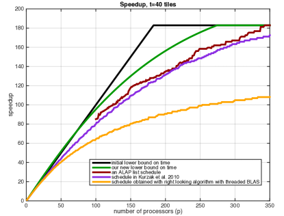
Figure 4: Speedup for a tiled Cholesky factorization with t=40 tiles. We plot two upper bounds (black and green curves) on the set of speedups obtained for all schedules. And we plot three speedups (red, purple and yellow curves) obtained by three schedules.

VI Conclusion

We have analyzed the tiled Cholesky factorization and improved existing lower bounds on the execution time of any schedule, with a technique that benefits from the structure of dependence graph of the tiled Cholesky factorization.

We took advantage of our observation that the tiled Cholesky factorization is much better behaved when we schedule it with an ALAP (As Late As Possible) heuristic than an ASAP (As Soon As Possible) heuristic.

We believe that our theoretical results will help practical scheduling studies of the tiled Cholesky factorization. Indeed, our results enable to better characterize the quality of a practical schedule with respect to an optimal schedule.

We also believe that our technique is generalizable to many tile algorithms, in particular LU and QR. It is clear that many linear algebra operations would benefit from the ALAP scheduling strategy. Also, we can easily change the weight of the tasks in our study to better represent the time of the kernels (as opposed to the number of flops of the kernels) on a given architecture.

There are two questions left open by our work. First we do not have satisfying closed form formula for schedules on $p$ processors. Indeed, in Section V, we relied on simulation to plot the speedup of an ALAP schedule and of the schedule from Kurzak et al. [7]. We do not have closed form formula for these. Also, while we made significant progress, there is still a gap between our lower and upper bounds and it seems worthwhile to further our work and close this gap in an asymptotic sense.

References

- [1] F. Gustavson, L. Karlsson, and B. Kågström, “Distributed SBP Cholesky factorization algorithms with near-optimal scheduling,” ACM T. Math. Software, vol. 36, no. 2, pp. 1–25, 2009.
- [2] J. Kurzak, A. Buttari, and J. Dongarra, “Solving systems of linear equations on the CELL processor using Cholesky factorization,” IEEE Trans. Parallel Distrib. Syst., vol. 19, no. 9, pp. 1175–1186, 2008.
- [3] E. Chan, F. G. Van Zee, P. Bientinesi, E. S. Quintana-Ortí, G. Quintana-Ortí, and R. van de Geijn, “Supermatrix: a multithreaded runtime scheduling system for algorithms-by-blocks,” in PPoPP ’08: Proceedings of the 13th ACM SIGPLAN Symposium on Principles and practice of parallel programming. New York, NY, USA: ACM, 2008, pp. 123–132.
- [4] E. Agullo, B. Hadri, H. Ltaief, and J. Dongarra, “Comparative study of one-sided factorizations with multiple software packages on multi-core hardware,” in SC’09. ACM/IEEE Conference on Supercomputing, Portland, OR, November, 2009.
- [5] F. Song, A. YarKhan, and J. Dongarra, “Dynamic task scheduling for linear algebra algorithms on distributed-memory multicore systems,” in SC’09. ACM/IEEE Conference on Supercomputing, Portland, OR, November, 2009.
- [6] E. Agullo, O. Beaumont, L. Eyraud-Dubois, J. Herrmann, S. Kumar, L. Marchal, and S. Thibault, “Bridging the gap between performance and bounds of Cholesky factorization on heterogeneous platforms,” in Heterogeneity in Computing Workshop 2015, 2015.
- [7] J. Kurzak, H. Ltaief, J. Dongarra, and R. M. Badia, “Scheduling dense linear algebra operations on multicore processors.” Concurrency and Computation: Practice and Experience, vol. 22, no. 1, pp. 15–44, 2010.
- [8] R. M. Badia, J. R. Herrero, J. Labarta, J. M. Pérez, E. S. Quintana-Ortí, and G. Quintana-Ortí, “Parallelizing dense and banded linear algebra libraries using SMPSs,” Concurrency and Computation: Practice and Experience, vol. 21, no. 18, pp. 2438–2456, 2009.
- [9] G. Bosilca, A. Bouteiller, A. Danalis, T. Herault, P. Lemarinier, and J. Dongarra, “DAGuE: A generic distributed dag engine for high performance computing,” Parallel Computing, vol. 38, no. (1-2), pp. 37–51, 2012.
- [10] T. Gautier, X. Besseron, and L. Pigeon, “KAAPI: A thread scheduling runtime system for data flow computations on cluster of multi-processors,” in PASCO’07, London, Ontario, Canada, Jul. 2007.
- [11] A. YarKhan, J. Kurzak, and J. Dongarra, “QUARK users’ guide: Queueing and runtime for kernels,” University of Tennessee, Innovative Computing Laboratory, Tech. Rep. ICL-UT-11-02, 2011.
- [12] C. Augonnet, S. Thibault, R. Namyst, and P.-A. Wacrenier, “StarPU: a unified platform for task scheduling on heterogeneous multicore architectures,” Concurrency and Computation: Practice and Experience, Special Issue: Euro-Par 2009, vol. 23, pp. 187–198, Feb. 2011.
- [13] J. M. Pérez, R. M. Badia, and J. Labarta, “A flexible and portable programming model for SMP and multi-cores,” Barcelona Supercomputing Center – Centro Nacional de Supercomputacioń, Tech. Rep., Jun. 2007.
- [14] E. S. Quintana-Ortí, G. Quintana-Ortí, R. A. van de Geijn, F. G. Van Zee, and E. Chan, “Programming matrix algorithms-by-blocks for thread-level parallelism,” vol. 36, no. 3, 2009.
- [15] M. Cosnard, M. Marrakchi, Y. Robert, and D. Trystram, “Parallel gaussian elimination on an MIMD computer,” Parallel Computing, vol. 6, no. 3, pp. 275–296, 1988.
- [16] Y. Robert and D. Trystram, “Optimal scheduling algorithms for parallel gaussian elimination,” Theoretical Computer Science, vol. 64, no. 2, pp. 159 – 173, 1989.
- [17] M. Marrakchi and Y. Robert, “Optimal algorithms for gaussian elimination on a MIMD computer,” Parallel Computing, vol. 12, pp. 183–194, 1989.