Timing Gamma-ray Pulsars with the Fermi Large Area Telescope: Timing Noise and Astrometry

Abstract

We have constructed timing solutions for 81 $\gamma$-ray pulsars covering more than five years of Fermi data. The sample includes 37 radio-quiet or radio-faint pulsars which cannot be timed with other telescopes. These timing solutions and the corresponding pulse times of arrival are prerequisites for further study, e.g. phase-resolved spectroscopy or searches for mode switches. Many $\gamma$-ray pulsars are strongly affected by timing noise, and we present a new method for characterizing the noise process and mitigating its effects on other facets of the timing model. We present an analysis of timing noise over the population using a new metric for characterizing its strength and spectral shape, namely its time-domain correlation. The dependence of the strength on $\nu$ and $\dot{\nu}$ is in good agreement with previous studies. We find that noise process power spectra $S(f)$ for unrecycled pulsars are steep, with strong correlations over our entire data set and spectral indices $S(f)\propto f^{-\alpha}$ of $\alpha\sim$5–9. One possible explanation for these results is the occurrence of unmodelled, episodic ‘microglitches’. Finally, we show that our treatment of timing noise results in robust parameter estimation, and in particular we measure a precise timing position for each pulsar. We extensively validate our results with multi-wavelength astrometry, and using our updated position, we firmly identify the X-ray counterpart of PSR J1418$-$6058.

1. Introduction

The Large Area Telescope (LAT, Atwood et al., 2009) of the Fermi Gamma-ray Space Telescope has now detected more than 150 pulsars, extending over six orders of magnitude in spin-down luminosity and divided roughly evenly between young ‘normal’ pulsars and ‘recycled’ millisecond pulsars (MSPs). The ‘normal’ population is further roughly equally divided into radio-loud and radio-quiet/radio-faint pulsars. See the 2nd Fermi Pulsar Catalog (2PC; Abdo et al., 2013) for a detailed analysis. This bonanza both probes the high-energy emission mechanism and offers selection effects appreciably different to those of radio surveys. E.g., the sensitivity of ‘blind searches’—efforts to detect $\gamma$-ray pulsations without a priori information about the period—for young pulsars suffers in the bright diffuse background of the Galactic plane (Dormody et al., 2011), while Fermi is particularly good at selecting MSP candidates whose pulsations can be detected with deep radio telescopes searches (e.g. Ransom et al., 2011; Kerr et al., 2012; Camilo et al., 2012b).

Important properties of pulsars, such as their frequency $\nu$, their spin-down rate $\dot{\nu}$, their position and proper motion, and their orbital parameters, can be determined through pulsar timing. This procedure—as old as pulsars themselves (Hewish et al., 1968)—both measures pulse times of arrival (TOAs) and models their generation and propagation so as to coherently account for every rotation of the neutron star. Measuring these parameters is key to understanding the distribution of pulsars within the Galaxy. Moreover, deviations from expectations often yield new insights, e.g. pulse nulling over very long time-scales (intermittency; Kramer et al., 2006; Camilo et al., 2012a), correlated shifts in pulse profile and spin-down luminosity (Lyne et al., 2010), and dramatic, rapid shifts in magnetospheric configuration (Hermsen et al., 2013). More recently, Allafort et al. (2013) presented the discovery of the first state switch observed in $\gamma$-rays, in which an abrupt increase of the spin-down rate $\dot{\nu}$ of PSR J2021$+$4026 was accompanied by both a decrease in total flux and change in pulse shape.

The efficacy of pulsar timing is reduced by timing noise (TN), a red noise process first recognized by Boynton et al. (1972). TN is intrinsic to pulsar rotation and operates over a broad range of time-scales. It is generally strongest in young pulsars (e.g. Shannon & Cordes, 2010), with noise processes whose amplitudes can be far larger than the pulsar period ($>$1 s), while TN in MSPs is much weaker, with amplitudes of order 1 $\upmu$s. Because TN cannot be modelled a priori, it confuses the deterministic signature of other parameters of interest. On the other hand, if TN can be definitely related to a particular physical mechanism (e.g. Cordes & Greenstein, 1981; Lyne et al., 2010), it provides another means of understanding neutron stars and their magnetospheres.

For Fermi pulsars, TN is the primary obstacle to identifying counterparts at other wavelengths. Because the angular resolution of the LAT is coarse compared to focusing telescopes, determining the counterpart of a $\gamma$-ray source typically requires the detection of correlated temporal variability (Nolan et al., 2012). On the other hand, pulsar timing offers an essentially interferometric localization with a baseline of up to 1 AU, with position errors inducing an annual sinusoidal modulation in the pulse TOAs. TN obscures and corrupts this signal, but a data set spanning years has multiple realizations of both the sinusoid and the annual-scale fluctuations of the noise process, allowing the signals to be disentangled. Thus, it behooves us to collect long sets of precise TOAs for each detected $\gamma$-ray pulsar.

As with modelling TN, measuring TOAs with Fermi also presents challenges. The LAT only collects a few photons per day from a typical $\gamma$-ray pulsar, and measurement of a single TOA requires integrations ranging from hours to months. Sources are embedded in the strong diffuse background and are sometimes confused with bright neighboring sources; both situations require sophisticated spectral modelling to optimize the pulsar signal. Finally, the LAT pulsar sample includes many young, energetic pulsars with strong TN and glitches. Glitches are sudden step changes in $\nu$ and $\dot{\nu}$, often with a transient component in which the increased spin-down rate “recovers” nearly to the pre-glitch value; see e.g. Espinoza et al. (2011) for a large sample of examples. All told, during the time required to obtain a single TOA, the phase of the neutron star may have drifted considerably, and one finds oneself in the unenviable position of needing the timing model to measure the timing model!

With the large pulsar population and the steady acquisition of more than five years of all-sky data, we are now in a position to better address both TN and TOA measurements. Building on the work of Ray et al. (2011), we have developed a suite of techniques for reliably measuring TOAs from Fermi data with maximum likelihood. By applying a relatively new approach, in which TN is modelled as correlations among TOAs (Coles et al., 2011, hereafter C11), we are able to accurately measure the TN component and obtain unbiased estimates for pulsar timing parameters. We have incorporated these techniques into a pipeline which provides updated timing solutions and TOAs for all $\gamma$-ray pulsars above a nominal flux threshold. These products—including, for the first time, TOAs—are freely available to the community. We expect them to be of interest to researchers for a variety of topics, including the construction of detailed folded light curves, population analyses, and searches for state changes.

We introduce the timing sample and the reduction of $\gamma$-ray and radio data in §2.1, 2.2, and 2.3, respectively. We describe the maximum likelihood-based timing pipeline and resulting data products in §2.4 and §2.5. In §3.1, we discuss in detail our approach to measuring TN. With those results, we present an analysis of TN in the $\gamma$-ray pulsar population (§3.2 and §3.3), in particular characterizing the strength and shape of the TN spectrum. Finally, we demonstrate the power of our method by determining reliable, precise timing positions for the sample in §4. Where appropriate, we discuss results in situ.

2. Analysis

2.1. Pulsar Sample

Our approximately flux-limited sample comprises 81 pulsars, including 36 radio-quiet or radio-faint pulsars which are too dim to time with modern radio telescopes, viz. PSRs J1124$-$5916 and J1907$+$0602. This sample represents a marked increase over the 16 pulsars characterized in Ray et al. (2011), with gains coming from both a larger pool of detected $\gamma$-ray pulsars and a flux threshold lower by a factor of about five.

The basic criterion for selection is that the pulse is reliably detected in the TOA integration interval. We selected as our maximum interval a span of 56 days which is approximately the precessional period of the Fermi spacecraft, on which the exposure to a source cycles. Because sharp pulses are more easily detected than broad ones, this detectability criterion does not translate directly into a flux cutoff. Empirically, if a pulsar can generate a weighted $H$-test statistic (Kerr, 2011; de Jager et al., 1989) of $\sim$15, about 3$\sigma$, during a given interval, it can be timed reliably at that cadence. We based our thresholds on the 2PC weighted $H$-test values, computed with three years of data: for a cadence of 56 days, pulsars reaching $H$$\sim$250 in three years satisfy the detection criterion. We were unable to obtain phase-connected timing solutions for a few pulsars surpassing this threshold, viz. J1838$-$0537, J0554$+$3107, J1810$+$1744, and J2043$+$2740, and these pulsars are excluded from the sample. These timing solutions may be recovered with unbinned timing techniques, improved Fermi event reconstruction, and/or contributions of radio TOAs.

We conclude with a few remarks on our choice of maximum cadence. As we describe below, extraction of a TOA requires a timing solution valid over the course of the integration period. In the case of young pulsars, both TN and glitches are prohibitive of long integration periods, with our experience leading us to adopt 56 days. On the other hand, MSPs, with their much more stable rotation, can benefit from even longer integration periods, effectively lowering the sample flux threshold. However, these longer integration periods prohibit timing of short time-scale features, e.g. the orbital period, requiring ancillary observations from radio telescopes to provide initial characterization. Ultimately, these issues demand an unbinned analysis, in which the timing model is fitted directly to photon timestamps. Because pulsar timing machinery is based on the concept of TOA, such a switch represents a major task for future workers.

2.2. LAT Data Reduction

We analyze 5.2 years of Source-class Pass 7 LAT data acquired between 2008 Aug 4 (MET 239557418) and 2013 Oct 21 (MET 404063018). We note that these data are “unreprocessed” (cf. Johnson et al., 2013), but that the improved properties of the reprocessed data have little benefit for pulsar timing. The data span nearly the entire period of the uniform Fermi all-sky survey, terminating only a month before the switch into a modified survey mode with enhanced exposure to the Galactic center and modestly compromised exposure elsewhere.

Using gtmktime (Fermi Science Tools version 09-31-02), we filtered events lying outside the Good Time Intervals defined by the Fermi-LAT team, which exclude the regular passages through the South Atlantic Anomaly and transient events such as bright solar flares. We also reject events when the rocking angle of the spacecraft exceeds $52^{\circ}$ and those with a zenith angle $>$100^∘; these cuts primarily eliminate background from $\gamma$-rays generated along the earth’s limb. To further reduce the background, primarily from the bright Galactic diffuse emission, we apply photon weighting (Kerr, 2011) with gtsrcprob using the P7SOURCE_V6 instrument response function. The photon weights (see §2.4 for application) are estimates of the probability that a given event arrives from the pulsar instead of the background, and require an estimate for the spectrum of each. For most pulsars, we use the 2PC spectral and background models. For four additional pulsars discovered in blind searches, PSRs J0554$+$3107, J1422$-$6138, J1522$-$5735, J1932$+$1916, we use the spectral models derived in Pletsch et al. (2013). Although spectral models may be derived with different data sets and instrumental representations than those employed here, the photon weights needed for timing analysis do not depend sensitively on the precision of the model (Kerr, 2011).

Finally, we select photons within 2$\arcdeg$ of the pulsar position with reconstructed energies lying between 100 MeV and 30 GeV. Where required, we make use of the Fermi plugin for Tempo2 (Hobbs et al., 2006) to assign pulse phase to these photons.

2.3. Radio Data Reduction

For a subset of our pulsars, we have obtained high-quality timing data from radio telescopes, primarily from ongoing programs to monitor high-$\dot{E}$ pulsars in support the Fermi mission (Smith et al., 2008). Most data come from the Parkes campaign (Weltevrede et al., 2010) and were reduced via a pipeline that performs polarimetric calibration and impulsive and narrowband RFI excision; the raw data are available through the CSIRO Data Archive Portal (Hobbs et al., 2011).

Two MSPs (J1902$-$5105 and J1514$-$4946) discovered in a Parkes survey were monitored for two years and we include the TOAs, produced and reduced as per Kerr et al. (2012), in our sample.

Two young pulsars, J1747$-$2958 and J1833$-$1034, are visible to Parkes but too dim to be reliably timed. These were monitored with the Green Bank Telescope for three years, and we likewise include these data.

Table 1Positions from Fermi timing and from multi-wavelength (MWL) observations for normal (‘unrecycled’) pulsars. All positions are computed at the epoch MJD 55555 (25 Dec 2010), and positions reported in the literature are advanced to this epoch, with propagation of error, when proper motions are available. The TOA cadence and best-fit timing noise models are also shown.
Astrometry references: ^aHalpern et al. (2004); ^bSlane et al. (2002); ^cDe Luca et al. (2011); ^dKaplan et al. (2008); ^eRay et al. (2011); ^fCaraveo et al. (1998); ^gFaherty et al. (2007); ^hBrisken et al. (2003); ⁱDodson et al. (2003); ^jKargaltsev et al. (2012); ^kKeith et al. (2008); ^lStappers et al. (1999); ^mGonzalez et al. (2006); ⁿMignani et al. (2010); ^oHughes et al. (2003); ^pMarelli (2012); ^qCamilo et al. (2004); ^rNg et al. (2005); ^sKargaltsev et al. (2008); ^jKargaltsev et al. (2012); ^eRay et al. (2011); ^tRomani et al. (2010); ^uGaensler et al. (2004); ^vVan Etten et al. (2012); ^eRay et al. (2011); ^wCamilo et al. (2006); ^xHalpern et al. (2002); ^yAbdo et al. (2010); ^AZeiger et al. (2008); ^jKargaltsev et al. (2012); ^BVan Etten et al. (2008); ^CWeisskopf et al. (2011); ^DCamilo et al. (2009); ^EHalpern et al. (2001)

Name	Cadence	TN Model	R.A.	Decl.	MWL R.A.	MWL Decl.
	(days)		(J2000.0)	(J2000.0)	(J2000.0)	(J2000.0)
J0007$+$7303	7	BPL	00h07m00$\fs$205 (2.382)	$+$73$\arcdeg$03$\arcmin$17$\farcs$46 (9.93)	00h07m01$\fs$560 (0.010)	$+$73$\arcdeg$03$\arcmin$08$\farcs$10 (0.10)a
J0106$+$4855	28	BPL	01h06m25$\fs$030 (0.046)	$+$48$\arcdeg$55$\arcmin$52$\farcs$01 (0.57)	–	–
J0205$+$6449	14	PL	02h05m35$\fs$985 (2.162)	$+$64$\arcdeg$49$\arcmin$32$\farcs$95 (15.76)	02h05m37$\fs$920 (0.020)	$+$64$\arcdeg$49$\arcmin$42$\farcs$80 (0.72)b
J0248$+$6021	56	BPL	02h48m18$\fs$642 (0.160)	$+$60$\arcdeg$21$\arcmin$34$\farcs$70 (1.50)	–	–
J0357$+$3205	14	BPL	03h57m52$\fs$161 (0.075)	$+$32$\arcdeg$05$\arcmin$23$\farcs$63 (3.37)	03h57m52$\fs$329 (0.017)	$+$32$\arcdeg$05$\arcmin$20$\farcs$73 (0.25)c
J0534$+$2200	7	BPL	05h34m31$\fs$889 (0.088)	$+$22$\arcdeg$01$\arcmin$18$\farcs$46 (24.76)	05h34m31$\fs$929 (0.004)	$+$22$\arcdeg$00$\arcmin$52$\farcs$16 (0.06)d
J0622$+$3749	56	FPL	06h22m10$\fs$411 (0.073)	$+$37$\arcdeg$49$\arcmin$14$\farcs$60 (3.49)	–	–
J0631$+$1036	56	BPL	06h31m27$\fs$369 (0.113)	$+$10$\arcdeg$37$\arcmin$05$\farcs$63 (7.03)	–	–
J0633$+$0632	7	BPL	06h33m44$\fs$136 (0.025)	$+$06$\arcdeg$32$\arcmin$29$\farcs$48 (1.30)	06h33m44$\fs$142 (0.020)	$+$06$\arcdeg$32$\arcmin$30$\farcs$40 (0.30)e
J0633$+$1746	14	BPL	06h33m54$\fs$288 (0.003)	$+$17$\arcdeg$46$\arcmin$15$\farcs$32 (0.44)	06h33m54$\fs$310 (0.003)	$+$17$\arcdeg$46$\arcmin$14$\farcs$60 (0.04)fg
J0659$+$1414	28	BPL	06h59m48$\fs$183 (0.005)	$+$14$\arcdeg$14$\arcmin$21$\farcs$54 (0.41)	06h59m48$\fs$180 (0.001)	$+$14$\arcdeg$14$\arcmin$21$\farcs$13 (0.00)h
J0734$-$1559	56	BPL	07h34m45$\fs$693 (0.028)	$-$15$\arcdeg$59$\arcmin$18$\farcs$43 (0.67)	–	–
J0835$-$4510	7	BPL	08h35m20$\fs$612 (0.116)	$-$45$\arcdeg$10$\arcmin$33$\farcs$98 (1.35)	08h35m20$\fs$560 ($<$0.001)	$-$45$\arcdeg$10$\arcmin$34$\farcs$55 ($<$0.01)i
J0908$-$4913	56	BPL	09h08m35$\fs$420 (0.023)	$-$49$\arcdeg$13$\arcmin$05$\farcs$79 (0.24)	09h08m35$\fs$393 (0.020)	$-$49$\arcdeg$13$\arcmin$04$\farcs$84 (0.30)j
J1016$-$5857	56	PL	10h16m21$\fs$266 (0.092)	$-$58$\arcdeg$57$\arcmin$11$\farcs$70 (0.71)	–	–
J1023$-$5746	7	BPL	10h23m02$\fs$388 (0.703)	$-$57$\arcdeg$46$\arcmin$09$\farcs$86 (5.39)	–	–
J1028$-$5819	7	BPL	10h28m27$\fs$888 (0.004)	$-$58$\arcdeg$19$\arcmin$06$\farcs$14 (0.03)	10h28m28$\fs$000 (0.100)	$-$58$\arcdeg$19$\arcmin$05$\farcs$20 (1.50)k
J1044$-$5737	14	BPL	10h44m32$\fs$791 (0.024)	$-$57$\arcdeg$37$\arcmin$19$\farcs$39 (0.17)	–	–
J1048$-$5832	7	BPL	10h48m12$\fs$391 (0.253)	$-$58$\arcdeg$32$\arcmin$02$\farcs$68 (1.85)	10h48m12$\fs$640 (0.040)	$-$58$\arcdeg$32$\arcmin$03$\farcs$75 (0.01)lm
J1057$-$5226	14	BPL	10h57m58$\fs$970 (0.007)	$-$52$\arcdeg$26$\arcmin$56$\farcs$52 (0.07)	10h57m58$\fs$978 (0.010)	$-$52$\arcdeg$26$\arcmin$56$\farcs$27 (0.15)n
J1124$-$5916	14	PL	11h24m39$\fs$174 (0.863)	$-$59$\arcdeg$16$\arcmin$15$\farcs$32 (6.83)	11h24m39$\fs$100 (0.100)	$-$59$\arcdeg$16$\arcmin$20$\farcs$00 (1.00)o
J1135$-$6055	28	BPL	11h35m08$\fs$428 (0.048)	$-$60$\arcdeg$55$\arcmin$36$\farcs$50 (0.35)	11h35m08$\fs$450 (0.100)	$-$60$\arcdeg$55$\arcmin$36$\farcs$99 (1.70)p
J1357$-$6429	56	BPL	13h57m02$\fs$349 (0.278)	$-$64$\arcdeg$29$\arcmin$31$\farcs$67 (2.09)	13h57m02$\fs$430 (0.020)	$-$64$\arcdeg$29$\arcmin$30$\farcs$20 (0.10)q
J1413$-$6205	14	BPL	14h13m30$\fs$135 (0.113)	$-$62$\arcdeg$05$\arcmin$37$\farcs$02 (0.94)	–	–
J1418$-$6058	7	PL	14h18m42$\fs$725 (0.134)	$-$60$\arcdeg$58$\arcmin$01$\farcs$89 (1.27)	14h18m42$\fs$700 (0.080)	$-$60$\arcdeg$58$\arcmin$03$\farcs$10 (0.40)r
J1420$-$6048	28	PL	14h20m08$\fs$163 (0.250)	$-$60$\arcdeg$48$\arcmin$15$\farcs$55 (2.32)	–	–
J1429$-$5911	28	BPL	14h29m58$\fs$564 (0.019)	$-$59$\arcdeg$11$\arcmin$36$\farcs$02 (0.18)	–	–
J1459$-$6053	14	BPL	14h59m30$\fs$222 (0.024)	$-$60$\arcdeg$53$\arcmin$19$\farcs$87 (0.25)	–	–
J1509$-$5850	28	BPL	15h09m27$\fs$153 (0.004)	$-$58$\arcdeg$50$\arcmin$56$\farcs$05 (0.05)	15h09m27$\fs$163 (0.020)	$-$58$\arcdeg$50$\arcmin$56$\farcs$12 (0.30)s
J1522$-$5735	56	BPL	15h22m05$\fs$226 (0.107)	$-$57$\arcdeg$35$\arcmin$00$\farcs$91 (1.19)	–	–
J1620$-$4927	28	BPL	16h20m41$\fs$594 (0.089)	$-$49$\arcdeg$27$\arcmin$36$\farcs$21 (1.70)	–	–
J1709$-$4429	7	BPL	17h09m42$\fs$834 (0.339)	$-$44$\arcdeg$28$\arcmin$59$\farcs$26 (9.41)	17h09m42$\fs$748 (0.000)	$-$44$\arcdeg$29$\arcmin$08$\farcs$37 (0.00)
J1718$-$3825	28	BPL	17h18m13$\fs$576 (0.024)	$-$38$\arcdeg$25$\arcmin$18$\farcs$56 (1.07)	17h18m13$\fs$541 (0.020)	$-$38$\arcdeg$25$\arcmin$17$\farcs$26 (0.30)j
J1732$-$3131	14	BPL	17h32m33$\fs$551 (0.031)	$-$31$\arcdeg$31$\arcmin$20$\farcs$85 (2.59)	17h32m33$\fs$551 (0.030)	$-$31$\arcdeg$31$\arcmin$23$\farcs$92 (0.50)e
J1741$-$2054	14	BPL	17h41m57$\fs$282 (0.026)	$-$20$\arcdeg$54$\arcmin$04$\farcs$11 (6.71)	17h41m57$\fs$280 (0.020)	$-$20$\arcdeg$54$\arcmin$11$\farcs$80 (0.30)t
J1746$-$3239	56	PL	17h46m55$\fs$143 (0.141)	$-$32$\arcdeg$39$\arcmin$36$\farcs$36 (9.67)	–	–
J1747$-$2958	28	BPL	17h47m15$\fs$869 (0.018)	$-$29$\arcdeg$58$\arcmin$00$\farcs$93 (1.97)	17h47m15$\fs$854 (0.004)	$-$29$\arcdeg$58$\arcmin$01$\farcs$38 (0.04)u
J1803$-$2149	56	BPL	18h03m09$\fs$632 (0.007)	$-$21$\arcdeg$49$\arcmin$00$\farcs$87 (3.66)	–	–
J1809$-$2332	14	BPL	18h09m50$\fs$227 (0.018)	$-$23$\arcdeg$32$\arcmin$12$\farcs$98 (14.41)	18h09m50$\fs$249 (0.030)	$-$23$\arcdeg$32$\arcmin$22$\farcs$67 (0.10)v
J1813$-$1246	14	BPL	18h13m23$\fs$768 (0.005)	$-$12$\arcdeg$46$\arcmin$00$\farcs$63 (0.40)	–	–
J1826$-$1256	7	BPL	18h26m08$\fs$570 (0.042)	$-$12$\arcdeg$56$\arcmin$33$\farcs$53 (3.05)	18h26m08$\fs$540 (0.010)	$-$12$\arcdeg$56$\arcmin$34$\farcs$60 (0.10)e
J1833$-$1034	28	BPL	18h33m33$\fs$612 (0.047)	$-$10$\arcdeg$34$\arcmin$07$\farcs$69 (3.20)	18h33m33$\fs$570 (0.020)	$-$10$\arcdeg$34$\arcmin$07$\farcs$50 (0.10)w
J1836$+$5925	14	FPL	18h36m13$\fs$661 (0.013)	$+$59$\arcdeg$25$\arcmin$29$\farcs$77 (0.11)	18h36m13$\fs$723 (0.017)	$+$59$\arcdeg$25$\arcmin$30$\farcs$05 (0.10)x
J1846$+$0919	56	FPL	18h46m25$\fs$864 (0.038)	$+$09$\arcdeg$19$\arcmin$48$\farcs$99 (1.08)	–	–
J1907$+$0602	7	PL	19h07m54$\fs$751 (0.044)	$+$06$\arcdeg$02$\arcmin$15$\farcs$79 (1.32)	19h07m54$\fs$760 (0.050)	$+$06$\arcdeg$02$\arcmin$14$\farcs$60 (0.70)y
J1932$+$1916	56	BPL	19h32m19$\fs$775 (0.063)	$+$19$\arcdeg$16$\arcmin$38$\farcs$06 (1.56)	–	–
J1952$+$3252	7	PL	19h52m58$\fs$181 (0.046)	$+$32$\arcdeg$52$\arcmin$40$\farcs$98 (0.72)	19h52m58$\fs$189 (0.001)	$+$32$\arcdeg$52$\arcmin$40$\farcs$40 (0.01)A
J1954$+$2836	28	BPL	19h54m19$\fs$144 (0.008)	$+$28$\arcdeg$36$\arcmin$04$\farcs$84 (0.12)	–	–
J1957$+$5033	28	FPL	19h57m38$\fs$391 (0.068)	$+$50$\arcdeg$33$\arcmin$21$\farcs$24 (0.69)	–	–
J1958$+$2846	14	BPL	19h58m40$\fs$064 (0.013)	$+$28$\arcdeg$45$\arcmin$54$\farcs$07 (0.22)	19h58m40$\fs$013 (0.020)	$+$28$\arcdeg$45$\arcmin$55$\farcs$12 (0.30)j
J2021$+$3651	7	BPL	20h21m05$\fs$501 (0.150)	$+$36$\arcdeg$51$\arcmin$03$\farcs$79 (2.15)	20h21m05$\fs$430 (0.030)	$+$36$\arcdeg$51$\arcmin$04$\farcs$63 (0.50)B
J2021$+$4026	14	BPL	20h21m30$\fs$496 (0.502)	$+$40$\arcdeg$26$\arcmin$53$\farcs$56 (6.16)	20h21m30$\fs$733 (0.020)	$+$40$\arcdeg$26$\arcmin$46$\farcs$04 (0.30)C
J2028$+$3332	28	FPL	20h28m19$\fs$876 (0.008)	$+$33$\arcdeg$32$\arcmin$04$\farcs$23 (0.12)	–	–
J2030$+$3641	56	FPL	20h30m00$\fs$241 (0.022)	$+$36$\arcdeg$41$\arcmin$27$\farcs$30 (0.29)	–	–
J2030$+$4415	56	BPL	20h30m51$\fs$396 (0.021)	$+$44$\arcdeg$15$\arcmin$38$\farcs$73 (0.26)	–	–
J2032$+$4127	7	BPL	20h32m12$\fs$932 (0.344)	$+$41$\arcdeg$27$\arcmin$22$\farcs$82 (4.47)	20h32m13$\fs$143 (0.024)	$+$41$\arcdeg$27$\arcmin$24$\farcs$54 (0.27)D
J2055$+$2539	28	FPL	20h55m48$\fs$948 (0.032)	$+$25$\arcdeg$39$\arcmin$58$\farcs$93 (0.62)	–	–
J2111$+$4606	28	BPL	21h11m24$\fs$125 (0.069)	$+$46$\arcdeg$06$\arcmin$30$\farcs$66 (0.71)	–	–
J2139$+$4716	56	BPL	21h39m55$\fs$878 (0.064)	$+$47$\arcdeg$16$\arcmin$13$\farcs$12 (0.68)	–	–
J2229$+$6114	7	BPL	22h29m05$\fs$262 (0.515)	$+$61$\arcdeg$14$\arcmin$08$\farcs$48 (3.96)	22h29m05$\fs$280 (0.070)	$+$61$\arcdeg$14$\arcmin$09$\farcs$30 (0.50)E
J2238$+$5903	14	BPL	22h38m28$\fs$089 (0.187)	$+$59$\arcdeg$03$\arcmin$43$\farcs$37 (1.46)	–	–

Table 2As Table 1 for millisecond (‘recycled’) pulsars.
Astrometry references: ^aDeller et al. (2008)

Name	Cadence	TN Model	R.A.	Decl.	MWL R.A.	MWL Decl.
	(days)		(J2000.0)	(J2000.0)	(J2000.0)	(J2000.0)
J0030$+$0451	28	FPL	00h30m27$\fs$4277 (0.0010)	$+$04$\arcdeg$51$\arcmin$39$\farcs$710 (0.035)	–	–
J0218$+$4232	56	FPL	02h18m06$\fs$3604 (0.0008)	$+$42$\arcdeg$32$\arcmin$17$\farcs$365 (0.015)	–	–
J0340$+$4130	56	BPL	03h40m23$\fs$2887 (0.0004)	$+$41$\arcdeg$30$\arcmin$45$\farcs$300 (0.012)	–	–
J0437$-$4715	28	FPL	04h37m15$\fs$9314 (0.0007)	$-$47$\arcdeg$15$\arcmin$09$\farcs$318 (0.008)	04h37m15$\fs$9309 ($<$0.0001)	$-$47$\arcdeg$15$\arcmin$09$\farcs$318 ($<$0.001)a
J0613$-$0200	28	FPL	06h13m43$\fs$9759 (0.0002)	$-$02$\arcdeg$00$\arcmin$47$\farcs$228 (0.010)	–	–
J0614$-$3329	28	NTN	06h14m10$\fs$3479 (0.0000)	$-$33$\arcdeg$29$\arcmin$54$\farcs$116 (0.001)	–	–
J0751$+$1807	56	FPL	07h51m09$\fs$1539 (0.0020)	$+$18$\arcdeg$07$\arcmin$38$\farcs$335 (0.154)	–	–
J1231$-$1411	28	NTN	12h31m11$\fs$3069 (0.0001)	$-$14$\arcdeg$11$\arcmin$43$\farcs$628 (0.003)	–	–
J1514$-$4946	58	FPL	15h14m19$\fs$1142 (0.0001)	$-$49$\arcdeg$46$\arcmin$15$\farcs$528 (0.003)	–	–
J1614$-$2230	28	FPL	16h14m36$\fs$5070 (0.0016)	$-$22$\arcdeg$30$\arcmin$31$\farcs$207 (0.120)	–	–
J1744$-$1134	56	FPL	17h44m29$\fs$4103 (0.0004)	$-$11$\arcdeg$34$\arcmin$54$\farcs$727 (0.031)	–	–
J1902$-$5105	56	FPL	19h02m02$\fs$8476 (0.0001)	$-$51$\arcdeg$05$\arcmin$56$\farcs$969 (0.002)	–	–
J1959$+$2048	56	FPL	19h59m36$\fs$7480 (0.0001)	$+$20$\arcdeg$48$\arcmin$14$\farcs$599 (0.002)	–	–
J2017$+$0603	28	FPL	20h17m22$\fs$7048 (0.0003)	$+$06$\arcdeg$03$\arcmin$05$\farcs$585 (0.008)	–	–
J2043$+$1711	56	FPL	20h43m20$\fs$8828 (0.0002)	$+$17$\arcdeg$11$\arcmin$28$\farcs$941 (0.005)	–	–
J2124$-$3358	28	FPL	21h24m43$\fs$8464 (0.0010)	$-$33$\arcdeg$58$\arcmin$44$\farcs$961 (0.028)	–	–
J2214$+$3000	56	FPL	22h14m38$\fs$8480 (0.0004)	$+$30$\arcdeg$00$\arcmin$38$\farcs$209 (0.007)	–	–
J2241$-$5236	56	FPL	22h41m42$\fs$0199 (0.0002)	$-$52$\arcdeg$36$\arcmin$36$\farcs$224 (0.003)	–	–
J2302$+$4442	56	NTN	23h02m46$\fs$9789 (0.0002)	$+$44$\arcdeg$42$\arcmin$22$\farcs$102 (0.003)	–	–

2.4. Pulsar Timing

As outlined above, obtaining pulse TOAs with Fermi is fundamentally different from the process traditionally followed in radio astronomy. In the latter case, TOAs can be obtained with observations generally lasting less than an hour, a time-scale on which TN is negligible. The resulting pulse profiles follow Gaussian statistics even in the low S/N case. Measuring a TOA is then simply a matter of cross-correlation with a known template. In contrast, the LAT data may comprise only a few source photons atop a strong background. A proper description of the data requires Poisson statistics, and measuring a TOA is achieved through analysis of the likelihood profile as we describe below.

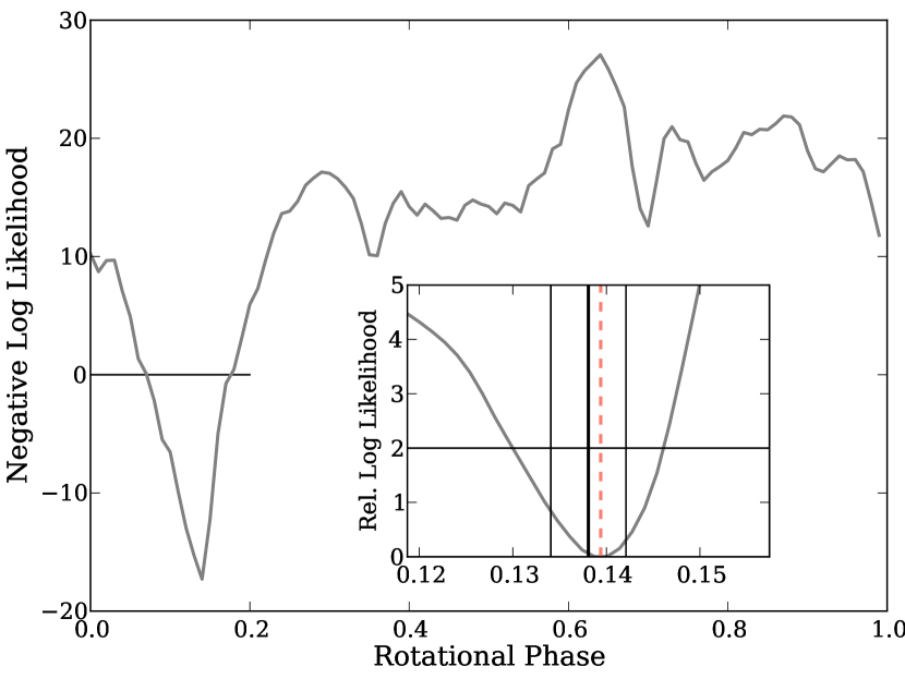
Figure 1.— The log likelihood as a function of relative phase between an analytic template and a pulse profile obtained from two weeks of data for PSR J0030$+$0451. There is a clear global extremum indicating a well-measured TOA. The log likelihood in the neighborhood of the extremum (inset) is asymmetric. As described in the text, instead of the extremum (dashed salmon line), we adopt the center of the interval defined by $\delta\log\mathcal{L}=2$ (solid black horizontal line). This TOA, and the corresponding error bounds, are shown as black vertical lines.

In measuring TOAs, we follow the method of Ray et al. (2011) with a few refinements. We use a weighted version of the likelihood, i.e. the probability density to observe a photon with phase $\phi$ given a pulse template $f(\phi)$ is $p(\phi)=wf(\phi)+(1-w)$, where $w$ is the photon weight computed above (§2.2). For TOAs with modest significance, the likelihood profile is often asymmetric, indicating the statistical uncertainty on the resulting TOA is also asymmetric. However, standard pulsar timing software, like the Tempo2 package we use, is predicated on Gaussian statistics and symmetric error bars. Thus, instead of simply using the likelihood maximum to measure a TOA, we determine a phase interval bounded by $\delta\log\mathcal{L}=2$ and we use the center of this interval and one-half of its width as estimators for the TOA and its uncertainty. We show an example for PSR J0030$+$0451 in Figure 1. Further, in order to avoid spurious TOA measurements, we require that the absolute value of the log likelihood exceeds five, a threshold we have determined empirically to work well. If there are multiple significant peaks in the likelihood, as is often the case for profiles with peaks separated by about half a rotation, we choose the peak closest to that predicted by the ephemeris.

We finally note that TOA extraction is an iterative process. Determing the photon phase $\phi$ over a TOA interval requires a valid timing solution, but this in turn requires a set of TOAs from which to determine a timing solution. We begin with an initial ephemeris that accurately tracks the pulsar rotational phase for some span of time (e.g. over three years from 2PC), and we extract TOAs using the method of Ray et al. (2011). The integration period for each TOA, which is uniform for a particular pulsar, varies from one week for the brightest pulsars in our sample to 56 days for the dimmest (see Tables 1 and 2).

Using the initial solution and TOAs, we jointly fit a new timing solution and a model for timing noise using the Cholesky factorization/generalized least squares method of C11 (see §3). Using the covariance matrix predicted by the best-fit TN model, we evaluate the TN process in the time domain with critical sampling (twice the TOA cadence). See Deng et al. (2012) for a similar application. With this new timing solution we extrapolate the pulse phase to the next interval of data and extract a new TOA. By repeating this process for each time step, we bootstrap a self consistent timing solution and set of TOAs.

We model glitches as sudden discontinuities in the spin-down model:

$$\phi(t) = \phi_{0}(t)+\theta(t-t_{g})\times$$ (1)

$$\big{\{} \phi_{g}+\delta\nu\,(t-t_{g})+\frac{1}{2}\delta\dot{\nu}\,(t-t_{g})^{2}+$$

$$\delta\nu_{d}\tau_{d}\,[1-\exp\frac{-(t-t_{g})}{\tau_{d}}]\big{\}},$$

where $t_{g}$ is the glitch epoch, $\theta$ is the Heaviside function, $\delta\nu$ and $\delta\dot{\nu}$ are permanent changes in the frequency and spin-down rate and $\delta\nu_{d}$ is a transient increase in the frequency exponentially decaying with time-scale $\tau_{d}$. New glitches are relatively easy to identify, as the pre-glitch timing solution will no longer produce a visible pulse profile when applied to post-glitch data. When we note such an occurrence, we estimate the epoch and then use unbinned likelihood to estimate the glitch parameters directly from the photon timestamps, fitting data collected for 90 d before and 180 d after the glitch. Empirically, we find that a subset of these parameters suffice to model the set of glitches. However, we also note that (1) generally we cannot access transient components with time-scales less than a few days (2) parameter estimates are affected by TN. Joint fitting of the glitch parameters and the TN model is beyond the current capability of our analysis and we leave this effort for future work, noting that the impact of fitting the glitch parameters independently does not appear to substantially alter the TN properties (see §3.3.2).

Once we have a timing solution spanning the full data set, we generate a new pulse profile and fit an analytic pulse template as described in 2PC. These templates are based on the 2PC models to which we have added minor components to model new features present in our augmented data set. For consistency, we use this new pulse profile to re-extract TOAs and fit a new timing solution. Although this ‘self standarding’ can lead to underestimates of TOA uncertainty (e.g. Hotan et al., 2005), we expect the effect to be minimal here because (1) we use an analytic template (2) our fitting is in the time domain.

2.5. Data Products

For each pulsar, the principal products of the pipeline are TOAs at an optimal cadence, a timing solution including a model of TN, and a pulse profile. These products—along with diagnostic plots—are public^, and generally updated every few months. The TN model, discussed below, is characterized by critically sampling its time domain realization (twice per TOA). This sampling is encoded in the timing solution via a set of IFUNC values, which specify the fixed points of a time series between which Tempo2 interpolates linearly. To compare these timing solutions with other published ephemerides and light curves, note that $\phi=0$ in our timing solutions corresponds to the leftmost bin of the corresponding profile.

3. Timing Noise

3.1. Maximum Likelihood Fitting

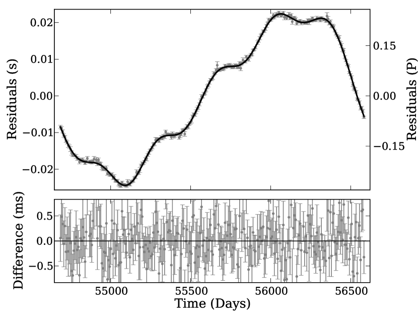
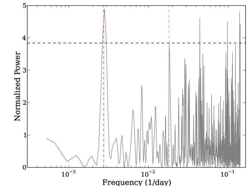
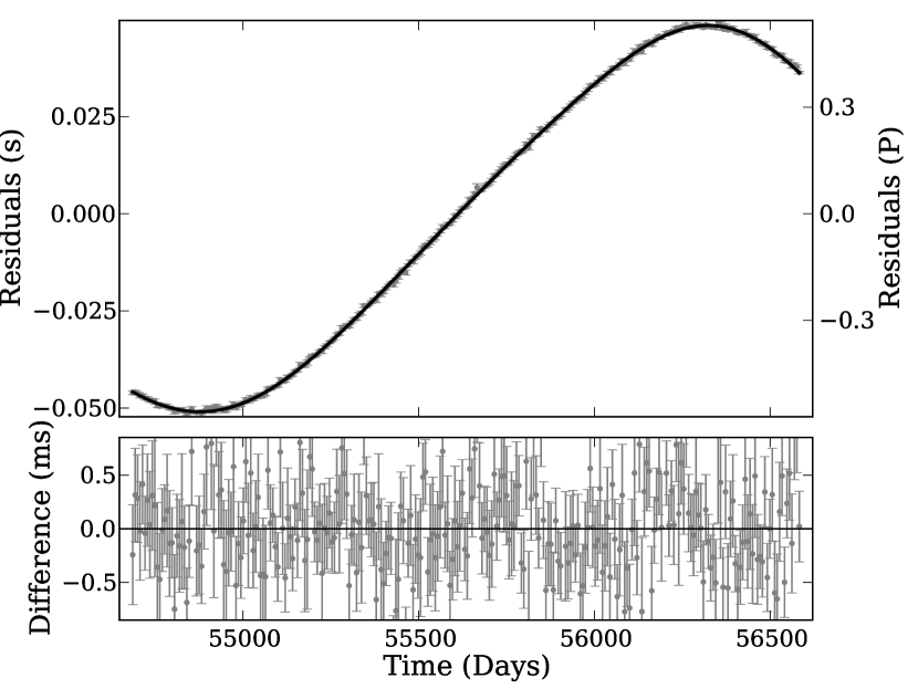
Figure 2.— Example of the TN fitting process for PSR J1028$-$5819. The top portions of the left-hand plots show the TOA residuals after a smooth spin-down model has been subtracted, as well as the estimated realization of the noise process (solid black line; see main text). Note that the dominant noise term is quadratic ($\dot{\nu}$-like). The lower portions of the left-hand plots show the difference between the TOA residuals and the noise estimator. The righthand plots show the power spectrum (as realized by the Lomb-Scargle periodogram) of the covariance-transformed residuals (see main text). The dashed horizontal line gives the amplitude that 5% of independent samples should surpass by chance, while the vertical salmon (green) line indicates periods of 365 and 55 days. In the top row, the position has been fixed at the independent ATCA position Keith et al. (2008). The offset from the timing position is statistically significant and the annual sinusoid appears superimposed on the realization of the red noise and excess power at the annual scale is clearly present in the periodogram. In the second row, the same plots appear after a joint fit of TN and position. The TN model has steepened to account for the reduced high frequency power, and accordingly the linear component ($\nu$-like) is strenghtened in the best-fit noise process. The annual power has vanished from the periodogram, which is largely consistent with white noise. Note the presence of aliasing in the higher frequencies of the periodograms.

Characterization of TN requires some model for the noise process. Historically, these models have included a Taylor expansion of the red noise realization through $\dot{\nu}$ and higher derivatives, and/or through harmonically related sinusoids (FITWAVES, Hobbs et al., 2004). With this approach, which models the realization of the noise process in the time domain, the measured TOAs remain statistically independent and maximum likelihood analysis is equivalent to weighted least squares (i.e., the covariance matrix is diagonal).

Unfortunately, C11 established that such ad hoc models of TN heavily bias other timing parameters, and instead those authors propose that the red noise process be modelled as widesense stationary, that is, that the correlations between TOAs are independent of time. Then, fitting can occur via generalized least squares by minimizing $\chi^{2}\equiv\mathbf{dx}^{\mathrm{T}}\,\mathbf{C}^{-1}\,\mathbf{dx}$, with juxtaposition indicating matrix multiplication, $\mathbf{C\equiv C_{meas}+C_{sto}}$, the combined covariance matrix of the white measurement (diagonal) errors and stochastic process (nondiagonal, symmetric), and $\mathbf{dx}$ being the residuals of the data with respect to the spin-down model only.

If the covariance matrix $\mathbf{C_{sto}}$ is chosen accurately—by which we mean the model reproduces the correlations observed in the TOA time series—then the above method provides optimal estimators for the timing parameters. C11 adopted a model in which the power spectrum of the TN is described in the frequency domain as a power law

$$S(f)=A^{2}[1+(f/f_{c})^{2}]^{-\alpha/2},$$ (2)

with the “corner frequency” $f_{c}$ providing a low-frequency saturation, $\alpha$ the spectral index, and $A$ the amplitude. They employed a spectral analysis of the residuals to the spin-down model to estimate these three parameters. The corner frequency was to some extent empirical because their fit was to the residuals, from which a quadratic term (viz. low frequency power) had already been removed by fitting $\nu$ and $\dot{\nu}$ (see e.g. van Haasteren & Levin, 2013). We also adopt this model for TN, but as we are interested both in the properties of the TN as well as its impact on other parameters, we choose to fit the TN parameters jointly with the spin-down model. This requires retaining the normalization term in the Gaussian likelihood; that is, denoting the stochastic TN parameters $\lambda_{s}$ and the pulsar spin-down parameters $\lambda_{p}$, we obtain parameter estimates by minimizing the quantity

$$-2\log\mathcal{L}\equiv\log\det\mathbf{C}(\lambda_{s})+\mathbf{dx}^{\mathrm{T}}(\lambda_{p})\,\mathbf{C}^{-1}(\lambda_{s})\,\mathbf{dx}(\lambda_{p}).$$ (3)

Moreover, we require the covariance matrix for the red noise process to be positive definite, in which case the total covariance matrix is necessarily positive definite, and we apply the Cholesky factorization $\mathbf{C}=\mathbf{L}^{\mathrm{T}}\,\mathbf{L}$, with $\mathbf{L}$ a lower triangular matrix. Thus, $\log\det\mathbf{C}$ reduces to $\sum_{i}\log L_{ii}$, and the “$\chi^{2}$” term can be written as $(\mathbf{L}^{-1}\,\mathbf{dx})^{\mathrm{T}}\,(\mathbf{L}^{-1}\,\mathbf{dx})$. For many pulsars with strong timing noise, the condition number of $\mathbf{C_{sto}}$ is untenably large and the Cholesky factorization greatly aids numerical stability.

To maximize $\log\mathcal{L}$ and characterize parameter uncertainties, we use Monte Carlo Markov chain sampling via emcee (Foreman-Mackey et al., 2013). For each proposed realization of power law parameters $\lambda_{s}$, we compute the covariance matrix for the $N\,(N-1)/2$ unique lags by computing the Fourier transform of $S(f)$; see Perrodin et al. (2013) for an analytic expression of the transform and note that this is essentially the well-known Matérn covariance function. If the matrix is positive definite, we factor it as described above. Otherwise we reject the sample. Next, we use the proposed set of spin-down parameters $\lambda_{p}$ together with Tempo2 to compute the residuals $\mathbf{dx}$. Finally, we compute $\log\mathcal{L}$ and return it to emcee to let it determine whether or not to accept the sample.

Because we have very little knowledge of the TN model a priori, we adopt broad priors on $\lambda_{s}$ by sowing the emcee “walkers” over a parameter space encompassing a large range of TN strengths and spectral shapes. Specifically, we use a prior uniform in the logarithm of $A^{2}$ from $-22$ to $12$, a uniform prior on $\alpha$ from 2 to 10, and a uniform prior on the logarithm of $f_{c}$ from $-5$ to $0$, with units on $A^{2}$ of s² d and units on $f_{c}$ of d^-1. Conversely, the timing model parameters are generally highly constrained, and we seed the walkers over a narrow parameter space centered on values from a Tempo2 fit with width of order the formal statistical uncertainties from the ordinary least squares fit. We then allow a lengthy burn-in for the walkers to “forget” their initial conditions and explore the covariance between $\lambda_{s}$ and $\lambda_{p}$. As long as the posterior distribution does not pile up on a boundary, we find our results are insensitive to the volume of the parameter space. We employ a basic spin-down model, fitting only $\nu$ and $\dot{\nu}$, save for the Crab pulsar, where $\ddot{\nu}$ is dynamically important and we also allow it to vary. For other pulsars, we fix $\ddot{\nu}=3\,\dot{\nu}^{2}/\nu$, i.e. assign a braking index of 3. For Crab, we include $\dddot{\nu}$ likewise fixed by the braking index prescription. If an arcsecond-precision position is not available from Chandra, optical telescopes, or VLBI measurements (see §4), or if the implied timing precision is much better than that of the multi-wavelength position, we also allow the position to vary. In Figure 2, we show one example where the systematic errors associated with an ATCA position for PSR J1028$-$5819 are clearly revealed in the timing analysis. Finally, the distribution of samples from emcee provide estimates of uncertainty on $\lambda$. If we have included radio TOAs, we fit an additional arbitrary phase offset between the Fermi and radio TOAs.

After this process, we have likelihood-maximizing parameters for the spin-down and TN model, but we still lack a time-domain realization of the noise process with which to generate a set of whitened residuals and thus an optimal timing solution. Deng et al. (2012) derive a maximum likelihood estimator for the noise process, but we find the required matrix inversion to be numerically unstable for pulsars with strong TN. Instead, we once again adopt an iterative process. According to the Karhunen-Loève theorem, the eigenvectors of $\mathbf{C_{sto}}$ are an optimal basis for an expansion of the noise process, and the coefficients of the expansion can be estimated by ordinary least squares to the timing residuals. (See, e.g., Tegmark et al. (1997) for an overview of Karhunen-Loève decomposition in an astronomical context.) We then approximate the noise process as a truncated Karhunen-Loève expansion, adding terms to the expansion until the fit becomes acceptable, i.e. the $\chi^{2}$ per degree of freedom is close to 1. This procedure is similar to that of FITWAVES, but we use a basis optimized to the noise process rather than a general harmonic basis. This realization of the noise process is included via linear interpolation in the publicly-available ephemerides.

3.2. Model Selection

Although fitting $\nu$ and $\dot{\nu}$ suppresses TN at time-scales comparable to the observation length (see van Haasteren & Levin, 2013), it is interesting to see if the joint fitting process preserves any evidence in support of noise processes with spectra well-described by power laws. We explore this by repeating the fitting process described above for a series of nested models in which

1. $A=0$ in Eq. 2; (no timing noise, ‘NTN’ in Tables 1 and 2);

2. $A>0$, $\alpha=3$, $f_{c}\ll 1/T$ (pure power law with fixed spectral index; ‘FPL’ in Tables 1 and 2);

3. $A>0$, $\alpha>0$, $f_{c}\ll 1/T$ (pure power law with free spectral index; ‘PL’ in Tables 1 and 2);

4. $A>0$, $\alpha>0$, $f_{c}>0$ (broken power law with low frequency cutoff, ‘BPL’ in Tables 1 and 2).

$T$ is the length of the data set, and the final case is precisely the fits described in the previous sections. Our choice of $\alpha=3$ represents red noise of modest steepness as an alternative to the steeper red noise we observe in the young pulsar sample. To select the optimal model, we apply the Akaike information criterion (Akaike, 1998), which requires $\delta\log\mathcal{L}>2$ to accept a model with an additional degree of freedom. The resulting classification for each pulsar appears in Tables 1 and 2, and in Figure 3.

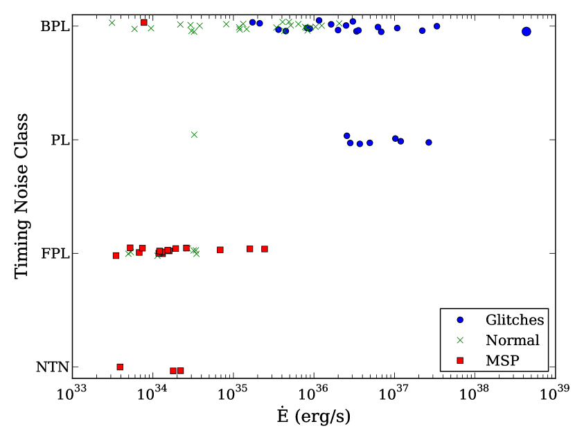
Figure 3.— The timing noise model classification (see main text and Tables 1 and 2) of each pulsar: Broken Power Law, (pure) Power Law, Fixed Power Law, and No Timing Noise. The points are staggered for visibility. The legend and symbols indicate three classes of pulsars: young pulsars having experienced a glitch (“Glitches”, blue circles); young pulsars without evidence glitches (“Normal”, green crosses); and millisecond pulsars (“MSP”, red squares). The symbol corresponding to the Crab pulsar, J0534$+$2200, is drawn slightly enlarged here and in subsequent figures.

Every young pulsar provides evidence for at least some level of TN, and for the vast majority, the preferred model is a broken power law. Curiously, the pulsars for which a pure power law (case 3 above) is optimal are mostly energetic, glitching pulsars. Because the glitches are not fit jointly with the TN or other spin parameters, they have a complicated effect on the spectrum. A data span $S$ (270 d) is used to determine the glitch parameters, and TN power with frequencies $>$$1/S$ will be reduced by the glitch fitting. On the other hand, inaccuracies in the permanent glitch parameters ($\delta\nu$ and $\delta\dot{\nu}$ in Eq. 1) appear as a step with asymptoptic spectrum $1/f^{2}$. Since this is much less steep than the intrinsic spectrum, however, the effect on the measured spectrum should be minor. Since pure power laws are preferred for glitching pulsars, this seems to be the case.

With one exception, at most a pure power law with fixed spectral index (case 2) is required to model the TN in MSPs. In fact, since the predicted red noise level (see below) is largely below the statistical precision of our TOAs, it is likely most of this “timing noise” is simply absorbing deficiencies in our white noise models, e.g. the likelihood asymmetry described in §3.1. This interpretation is reinforced in the case of PSR J1231$-$1411, which is the brightest known Fermi MSP, and thus least affected by issues with low statistical significance. Its optimal model requires no TN at all (case 0).

3.3. Measurements and Discussion

Substantial progress has been made in understanding the properties and underlying mechanisms of timing noise through the study of large samples of pulsars timed over many years, (e.g. Cordes & Helfand, 1980; Cordes & Downs, 1985; D’Alessandro et al., 1995; Hobbs et al., 2010b). The collection of pulsars timed here is comparable in both size and duration to many of these studies. Moreover, since the beams of $\gamma$-ray pulsars illuminate more of the sky than those of radio pulsars (e.g. Watters & Romani, 2011), the LAT sample may offer a less biased view of high-$\dot{E}$ pulsars. Both circumstances motivate an analysis and discussion of two key TN metrics, viz its strength and its spectral shape.

3.3.1 Amplitude

The strength of TN is a key parameter, as it sets the physical scale of the underlying noise process(es) and limits the precision with which deterministic parameters can be measured. Several metrics are available, including the best-fit value of $\ddot{\nu}$, the rms (root mean square) after fitting a low-order polynomial, and the $A$ parameter of Eq. 2. Because the latter is highly correlated with $f_{c}$, we adopt as a proxy for TN strength the integral timing noise $\int S(f)\,df$ or, equivalently, the zero-lag element of the time-domain covariance. To account for the statistical uncertainty in this quantity, we compute it using each entry of our Markov chain and report the mode and 68% central interval as a function of $\dot{E}$ in Figure 4. As extensively noted in the literature, as well as in our sample, the TN strength is highly correlated with $\dot{\nu}$ and mildly correlated with $\nu$, e.g. (Cordes & Helfand, 1980; Arzoumanian et al., 1994; Hobbs et al., 2010b), though see also Shannon & Cordes (2010). For uniformity of presentation, we use $\dot{E}$ as a proxy for $\dot{\nu}$ and other combinations of $\nu$ and $\dot{\nu}$. Interestingly, the Crab pulsar (J0534$+$2200) shows an anomalously low TN amplitude. Among young and energetic pulsars, it is unique in its proclivity for small glitches with complex recoveries (Espinoza et al., 2011), and it is no surprise its TN properties are out of family. Moreover, the Crab is the only pulsar for which we fit $\ddot{\nu}$.

Figure 4.— The amplitude of the timing noise process as estimated from the zero-lag autocorrelation of the best-fit TN model. Normal pulsars are classified according to those that do or do not suffer glitches. The central values and error bars displayed here and in subsequent figures with TN metrics are obtained from the central 68% of the Monte Carlo realizations described in the main text. Pulsars with undetectable levels of timing noise are shown without error bars at 1 $\mu$s amplitude.

By examining a large sample of pulsars, Shannon & Cordes (2010) identified a single relation spanning MSPs, young pulsars, and magnetars: $\sigma^{2}_{2}\propto\nu^{-1.8}\dot{\nu}^{2}$, where $\sigma_{2}$ is the rms scatter of the TOA residuals after fitting for $\nu$ and $\dot{\nu}$, with the subscript reminding that the model includes two and only two spin-down terms. Measurements of $\sigma_{2}$ for the pulsar population and the predictions of Shannon & Cordes (2010) are shown in Figure 5; observations in agreement with the relation lie along the diagonal dashed line. These values are obtained by measuring the rms scatter relative to a timing solution with $\nu$ and $\dot{\nu}$ and for which the best-fit noise process is either included in the model (“white rms”) or excluded from the model (“total rms”). Generally, the total rms (colored points in Figure 5) dwarfs the white rms (white points) for young pulsars, and the former can be taken as a proxy of the rms due to TN. However, as measurement noise becomes important, the two quantities approach equality, and we cannot reliably estimate the TN contribution. Although the values are in reasonable agreement with the fit, the LAT sample shows a steeper dependence on $\dot{\nu}$, more in keeping with the $\sigma^{2}_{2}\propto\nu^{-0.8}\dot{\nu}^{1.5}$ relation found by Hobbs et al. (2010a) in a fit to only typical unrecycled pulsars. In both cases, the white noise level of the MSP sample is well above the TN prediction.

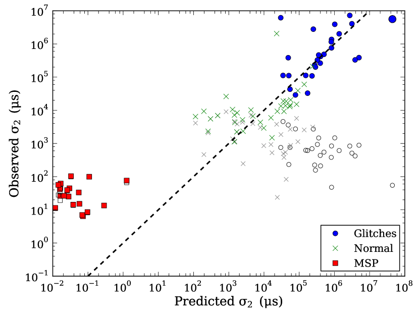
Figure 5.— The residual scatter after modelling $\nu$ and $\dot{\nu}$, $\sigma_{2}$ (see main text). The total scatter is depicted by larger colored points, while below them, estimates for the sample rms with the contribution of TN removed appear as smaller gray and white points. The x-axis gives the prediction from the scaling relation of Shannon & Cordes (2010), and the dashed line shows equality, i.e. agreement with this model. For pulsars with well-measured TN (colored points well above white points), the observations are in reasonable agreement.

It is interesting to compare our model-derived metric (Figure 4) with the sample rms in the case where we do not model TN. We expect that the primary difference will be the joint fit of the TN model with $\nu$ and $\dot{\nu}$, potentially allowing more noise to be associated with the TN model. Indeed, in Figure 6, we observe a tight but nonlinear correlation, with the TN predicted by our fit growing more quickly than the sample rms. The Crab pulsar lies more in trend with the $\sigma_{2}$ metric, which likely reflects the inclusion of a dynamic $\ddot{\nu}$ in the fit with which the TN amplitude is obtained.

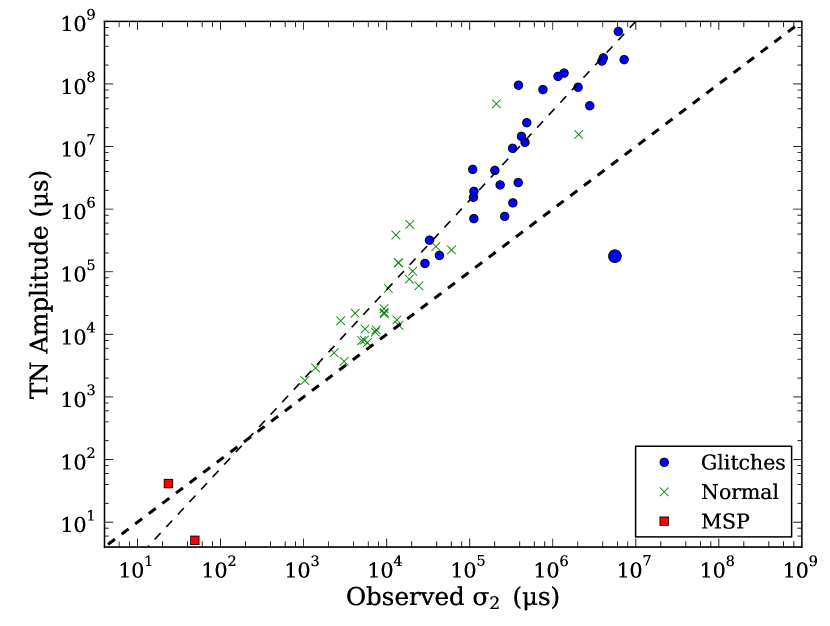
Figure 6.— The timing noise strength, as in Figure 4, as a function of the total rms, as per Figure 5. The heavy dashed line indicates a linear relation, while the steeper, lighter line has a (log log) slope of 7/5. Pulsars with undetectable timing noise are suppressed in this plot (see Figure 4).

3.3.2 Spectrum

The second important property of TN—and the one that offers insight into the physical mechanism(s)—is the degree of correlation over long time-scales, or equivalently, the steepness of the power spectrum of the TOA residuals. Like the amplitude parameter, $\alpha$ is highly correlated with $f_{c}$, and we prefer an empirical measure. We adopt the time required for the correlation to drop to one half of its peak (zero lag) value, which we call the correlation time-scale, and as before we make use of the Monte Carlo sampling to estimate values and uncertainties. These results appear in Figure 7 and show a very marked “redder when stronger” relation. Discounting the MSPs, the relationship is nearly a power law, though there is evidence for a break around 5 yr, the length of the data set, $T$. Correlation time-scales $>T$ are of course extrapolations and can be interpreted as statements that the data exhibit strong correlations over the entire range of observations. Because we only have one realization of the data with frequencies $\sim 1/T$, and because this portion of the spectrum dominates the total TN for steep spectra, precise characterization of these quantities at these time-scales is not possible.

Interestingly, though, this “saturation” time-scale is also the time-scale at which most pulsars experience strong glitches, so it is unclear if the saturation is due to glitches or absorption of red noise by $\nu$ and $\dot{\nu}$. Because the correlation time-scale is so strongly correlated with the TN amplitude, it is likewise strongly correlated with $\dot{E}$, as seen in Figure 8.

Figure 7.— The autocorrelation of the residuals (the Fourier transform of Eq. 2) monotonically decreases from zero lag. Shown here is the time required for the autocorrelation to drop to one half of its peak value, plotted as a function of timing noise strength. The black, dashed line indicates 5.2 yr, the length of the data set, and the clear trend appears to break modestly at this threshold.

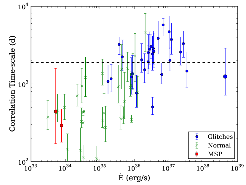
Figure 8.— As Figure 7 but with $\dot{E}$ for abscissa. The correlation time-scale increases monotonically with spin-down luminosity, save for a possible saturation/break at the highest values of $\dot{E}$.

As with TN strength, it is worth comparing our choice of the correlation time-scale with other metrics of the TN spectrum. The obvious choice, $\alpha$, is directly comparable to spectral analyses based on Fourier transforms, though we note the method employed here is immune to spectral leakage and we easily recover extremely steep spectra: our measurements of $\alpha$ appear in Figure 9. However, because of the correlation with $f_{c}$, $\alpha$ does not tell the full story and the strong correlation with $\dot{E}$ has vanished. Indeed, the most energetic pulsars may show a decrease in spectral index! In the time domain, on the other hand, the correlation increases monotonically with $\dot{E}$. We thus caution that, in studies of TN of young pulsars, careful attention should be paid to the metric employed.

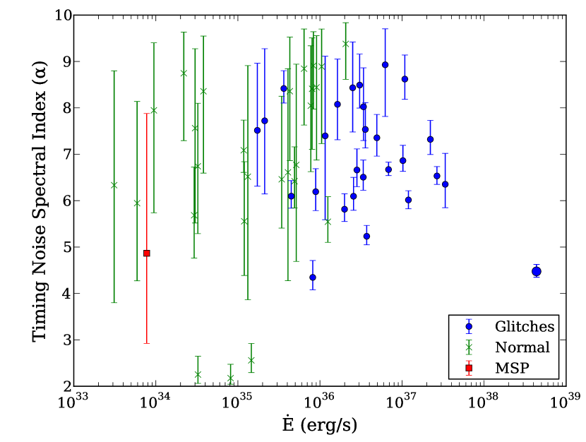
Figure 9.— The TN spectral index, $\alpha$. The spectra are nearly universally steep, with values of 5–9, with little evidence for dependence on $\dot{E}$.

On the other hand, the use of $\alpha$ allows us to make better contact with the literature. In the earliest studies of timing noise, it was realized that (under the assumption that the ‘step rate’ is fast enough), simple random walk processes would manifest as power law spectra. In particular, for a random walk in phase, $\alpha=2$; for $\nu$, $\alpha=4$; and for $\dot{\nu}$, $\alpha=6$. In a famous example, Boynton et al. (1972) determined the spectral index of the Crab pulsar, based on two years of timing data, to be $\approx 4$, consistent with our results here, and proposed its noise was largely ‘frequency jitter’. However, the majority of our pulsars show much steeper spectra, with typical values of 6–7 for the most energetic, glitching pulsars, and a broad range 5–9 for less energetic glitching and non-glitching young pulsars. As noted before, the TN properties of the MSPs in our sample are poorly constrained.

We conclude this section with a few remarks on the interplay between glitches and the (possibly) smooth noise process(es). In the case of large, resolved glitches, we expect we may be able to cleanly separate the effects (e.g. Alpar et al., 1986), and indeed we observe no systematic differences between the glitching and non-glitching populations save the ‘normal’ evolution with $\dot{E}$ and a tendency to favor pure power laws. On the other hand, while Espinoza et al. (2014) clearly show a minimum threshold for glitch amplitudes of the Crab pulsar, there is no corresponding result for the general population, and glitch amplitudes may stretch well into the ‘measurement noise’ resulting from both TOA precision and cadence. Indeed, Cordes & Downs (1985) found ‘microglitches’ to be an important factor in TN. These episodic jumps in $\nu$ and $\dot{\nu}$ were too large to be consistent with high-rate stochastic processes but were too small and with the incorrect sign for $\delta\nu$ to be true glitches. Such events are of particular concern for the LAT: they may be the hallmark of mode changes (Allafort et al., 2013), but the typical TOA precision and cadence are poor for many pulsars. A thorough analysis of this phenomenon requires new capabilities to jointly model glitches and TN, as well as to determine the sensitvity of Fermi to the former. We leave this challenging task to future work.

4. Astrometry

Pulsar timing can furnish extremely precise positions relative to the dynamical frame of the Solar System ephemeris, in this work typically realized by JPL DE405. For PSRs J0437$-$4715 and J2241$-$5236, we use the DE414 ephemeris, while for PSRs J1057$-$5226 and J2043$+$1711 we make use of the DE421 ephemeris. While small errors from frame transfer or from clock drifts are important for MSP positions, the dominant source of error for young pulsars is bias from TN (see e.g. Weisskopf et al., 2011; Ray et al., 2011). For multi-wavelength followup—e.g. deep searches for radio pulsations or X-ray searches for point sources—accurate positions with robust uncertainties are required.

Here, we show that our models of TN, together with Monte Carlo sampling (described above), provide the needed level of accuracy. To estimate the timing position uncertainties, we compute the Monte Carlo sample covariance in R.A. and Decl., obtaining the position error ellipse marginalized over all other parameters. Typically, correlation in R.A. and Decl. is small, and we simply report the 68% (“1 $\sigma$”) containment intervals for each coordinate.

To check these uncertainty estimates in the case of normal pulsars (affected by TN), we have collected from the literature all available precisely-measured pulsar positions, primarily from Chandra observations, but including some VLBI measurements and optical observations. We have intentionally excluded positions available from pulsar timing as they are subject to the same potential biases as our analysis. The positions, along with their provenance and uncertainty, are given in Tables 1 and 2. The Chandra position uncertainties, in particular, are heterogeneous, as the level of analysis ranges from none to a careful accounting of uncertainties due to photon counting, pointing aspect solution, and frame tie. For MSPs, the only positions with sufficient precision to be useful for comparison are obtained with VLBI, and we do not report positions with lesser precision.

To compare the timing positions with the independent literature positions, we referenced all timing positions to MJD 55555, while, for sources with reliable proper motions, we advanced the independent positions to the same epoch. The resulting coordinate differences, scaled to $\sigma^{2}=\sigma^{2}_{\mathrm{LAT}}+\sigma^{2}_{\mathrm{MWL}}$, i.e. the errors added in quadrature, are shown in Figure 10. The errors cluster within one unit without piling up at the origin, indicating that the timing position ellipse overlaps the multi-wavelength one without being overly conservative. Likewise, the Fermi data indicate no additional component of proper motion to within our measurement precision.

The one significant outlier is Geminga (PSR J0633$+$1746), whose Decl. is in agreement but whose R.A. differs by 5$\sigma$. Here, its absolute R.A. is taken from the Hubble and Hipparcos measurements of Caraveo et al. (1998) as 06^h33^m54$\fs$1530$\pm$0$\fs$0028 with an epoch of MJD 49793.5, while the angular proper motion $\mu_{\alpha}\cos\delta$ is measured with Hubble by Faherty et al. (2007) as $142.2\pm 1.1$ mas/yr. At the Fermi epoch MJD 55555, the total change in angle is $2\farcs 245\pm 0\farcs 017$, or a coordinate change of $0\fs 157\pm 0\fs 001$, giving a final position 06^h33^m54$\fs$310$\pm$0$\fs$003. This differs from the Fermi position by $0\fs 022$, or $0\farcs 31$. Accounting for the discrepancy requires either a 15% systematic error on the measured proper motion, or a systematic error of 300 mas in the optical frame tie; the latter seems more likely.

The statistical uncertainty estimates for our positions are clearly sufficiently accurate. Moreover, we can limit the absolute level of any systematic error within our timing chain itself by comparing the Fermi-only timing position of MSPs with precise VLBI positions. In the case of PSR J0437$-$4715, the timing position is in perfect agreeement with the 1-mas precision VLBI position of Deller et al. (2008), limiting any systematic errors to $<$10 mas. Several Fermi-LAT MSP positions have $\sim$mas precision, e.g. J0614$-$3329 and J1231$-$1411 (and see Figure 11), but those sources currently lack VLBI positions for comparison.

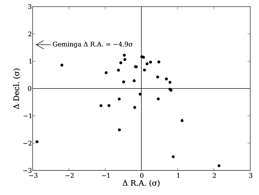
Figure 10.— The difference between the timing and multi-wavelength positions of Tables 1 and 2 in “$\sigma$” units, i.e. the timing and multi-wavelength errors summed in quadrature (see main text).

Although the positions above are unbiased, it is interesting to explore the degree to which TN degrades the possible precision. In Figure 11, we show the estimated precision in the R.A. coordinate as a function of both the total and white-only rms. In general, the MSPs and a few of the less energetic young pulsars track the ideal relation of $\sigma_{\mathrm{R.A.}}\propto\sigma_{\mathrm{TOA}}$. On the other hand, when TN becomes important, the position precision worsens by orders of magnitude. Interestingly, if we instead examine the precision as a function of the sample rms, which includes the effects of TN, we see that the position uncertainty is still highly correlated with the rms, but with an approximate $\sigma_{\mathrm{R.A.}}\propto\sqrt{\mathrm{rms}}$ relation. Essentially, the TN has destroyed the coherence of the position measurement. Thus, in the TN-dominated régime, we expect the position uncertainty to only improve as $1/\sqrt{t}$, while those pulsars free of TN (relative to the TOA precision) will enjoy a $1/t$ improvement in localization. We note that the best-measured positions of young pulsars have precisions of $<$100 mas, e.g. J1028$-$5819, suggesting that proper motion measurements may be feasible with longer data sets.

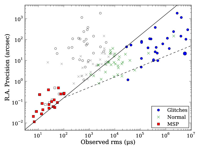
Figure 11.— The estimated precision on R.A. as a function of the observed scatter, as per Figure 5, save that here we indicate the “white noise” rms with gray, unfilled smaller markers, while the colored larger ones give the sample rms. The solid line indicates a linear relationship and indicates the best R.A. precision possible for the given white noise level. The dashed line follows $\sqrt{\mathrm{rms}}$.

We conclude with a case study of the power of robust position measurements. A prior attempt by Ray et al. (2011) to identify the X-ray counterpart of PSR J1418$-$6058, a radio-quiet pulsar embedded in the “Rabbit” pulsar wind nebula, could not discriminate between two Chandra point sources dubbed “R1” and “R2” (Ng et al., 2005). Although their timing position had sufficient formal statistical precision, its centroid was substantially biased by TN and consistent with neither X-ray source. With appreciably more data and a reliable TN model, we achieve a position uncertainty of $<$1″ and can firmly identify “R1” as the X-ray counterpart (Figure 12).

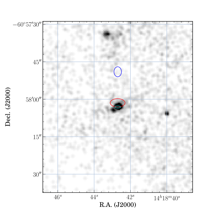
Figure 12.— The timing position of the radio-quiet PSR J1418$-$6058—given by the larger, red ellipse—agrees well with the Chandra X-ray position obtained by Ng et al. (2005), shown as the smaller, cyan ellipse. The timing position of Ray et al. (2011) is shown with the blue ellipse offset to the north of the Chandra source. The archival Chandra image (obs. 7640) has been smoothed with a Gaussian kernel of two pixels and the pointing aspect has not been corrected.

5. Summary and Conclusions

We have presented results of timing a large sample of both radio-quiet and radio-loud $\gamma$-ray pulsars with a long span of Fermi data. The strong TN in young pulsars required development of a new method in which a model for the stochastic TN process is fit jointly with the pulsar parameters, allowing characterization of the former and unbiased estimation of the latter. By comparing our best-fit timing positions with precise results from the literature, we demonstrated the efficacy of the method and were able to resolve a longstanding ambiguity in the X-ray counterpart of PSR J1418$-$6058. Our study of the TN properties indicates the spectra are generally quite steep and may reflect an unmodelled glitch contributions—e.g. recoveries from glitches both preceding and during our acquisition, or glitches below detection thresholds, i.e. ‘microglitches’.

The methods presented here are effective for more than half of the Fermi pulsar sample. Newly detected pulsars, however, will predominantly be fainter than those analyzed here and may not be amenable to TOA extraction. We hope the interesting results from this work spur the community to develop the techniques required for “photon-based” pulsar timing which would allow any $\gamma$-ray pulsar to be so characterized.

References

- Abdo et al. (2010) Abdo, A. A., Ackermann, M., Ajello, M., et al. 2010, ApJ, 711, 64
- Abdo et al. (2013) Abdo, A. A., Ajello, M., Allafort, A., et al. 2013, ApJS, 208, 17
- Akaike (1998) Akaike, H. 1998, in Selected Papers of Hirotugu Akaike (Springer), 199–213
- Allafort et al. (2013) Allafort, A., Baldini, L., Ballet, J., et al. 2013, ApJ, 777, L2
- Alpar et al. (1986) Alpar, M. A., Nandkumar, R., & Pines, D. 1986, ApJ, 311, 197
- Arzoumanian et al. (1994) Arzoumanian, Z., Nice, D. J., Taylor, J. H., & Thorsett, S. E. 1994, ApJ, 422, 671
- Atwood et al. (2009) Atwood, W. B., Abdo, A. A., Ackermann, M., et al. 2009, ApJ, 697, 1071
- Boynton et al. (1972) Boynton, P. E., Groth, E. J., Hutchinson, D. P., et al. 1972, ApJ, 175, 217
- Brisken et al. (2003) Brisken, W. F., Thorsett, S. E., Golden, A., & Goss, W. M. 2003, ApJ, 593, L89
- Camilo et al. (2012a) Camilo, F., Ransom, S. M., Chatterjee, S., Johnston, S., & Demorest, P. 2012a, ApJ, 746, 63
- Camilo et al. (2006) Camilo, F., Ransom, S. M., Gaensler, B. M., et al. 2006, ApJ, 637, 456
- Camilo et al. (2004) Camilo, F., Manchester, R. N., Lyne, A. G., et al. 2004, ApJ, 611, L25
- Camilo et al. (2009) Camilo, F., Ray, P. S., Ransom, S. M., et al. 2009, ApJ, 705, 1
- Camilo et al. (2012b) Camilo, F., Kerr, M., Ray, P. S., et al. 2012b, ApJ, 746, 39
- Caraveo et al. (1998) Caraveo, P. A., Lattanzi, M. G., Massone, G., et al. 1998, A&A, 329, L1
- Coles et al. (2011) Coles, W., Hobbs, G., Champion, D. J., Manchester, R. N., & Verbiest, J. P. W. 2011, MNRAS, 418, 561
- Cordes & Downs (1985) Cordes, J. M., & Downs, G. S. 1985, ApJS, 59, 343
- Cordes & Greenstein (1981) Cordes, J. M., & Greenstein, G. 1981, ApJ, 245, 1060
- Cordes & Helfand (1980) Cordes, J. M., & Helfand, D. J. 1980, ApJ, 239, 640
- D’Alessandro et al. (1995) D’Alessandro, F., McCulloch, P. M., Hamilton, P. A., & Deshpande, A. A. 1995, MNRAS, 277, 1033
- de Jager et al. (1989) de Jager, O. C., Raubenheimer, B. C., & Swanepoel, J. W. H. 1989, A&A, 221, 180
- De Luca et al. (2011) De Luca, A., Marelli, M., Mignani, R. P., et al. 2011, ApJ, 733, 104
- Deller et al. (2008) Deller, A. T., Verbiest, J. P. W., Tingay, S. J., & Bailes, M. 2008, ApJ, 685, L67
- Deng et al. (2012) Deng, X. P., Coles, W., Hobbs, G., et al. 2012, MNRAS, 424, 244
- Dodson et al. (2003) Dodson, R., Legge, D., Reynolds, J. E., & McCulloch, P. M. 2003, ApJ, 596, 1137
- Dormody et al. (2011) Dormody, M., Johnson, R. P., Atwood, W. B., et al. 2011, ApJ, 742, 126
- Espinoza et al. (2014) Espinoza, C. M., Antonopoulou, D., Stappers, B. W., Watts, A., & Lyne, A. G. 2014, MNRAS, 440, 2755
- Espinoza et al. (2011) Espinoza, C. M., Lyne, A. G., Stappers, B. W., & Kramer, M. 2011, MNRAS, 414, 1679
- Faherty et al. (2007) Faherty, J., Walter, F. M., & Anderson, J. 2007, Ap&SS, 308, 225
- Foreman-Mackey et al. (2013) Foreman-Mackey, D., Hogg, D. W., Lang, D., & Goodman, J. 2013, PASP, 125, 306
- Gaensler et al. (2004) Gaensler, B. M., van der Swaluw, E., Camilo, F., et al. 2004, ApJ, 616, 383
- Gonzalez et al. (2006) Gonzalez, M. E., Kaspi, V. M., Pivovaroff, M. J., & Gaensler, B. M. 2006, ApJ, 652, 569
- Halpern et al. (2001) Halpern, J. P., Camilo, F., Gotthelf, E. V., et al. 2001, ApJ, 552, L125
- Halpern et al. (2004) Halpern, J. P., Gotthelf, E. V., Camilo, F., Helfand, D. J., & Ransom, S. M. 2004, ApJ, 612, 398
- Halpern et al. (2002) Halpern, J. P., Gotthelf, E. V., Mirabal, N., & Camilo, F. 2002, ApJ, 573, L41
- Hermsen et al. (2013) Hermsen, W., Hessels, J. W. T., Kuiper, L., et al. 2013, Science, 339, 436
- Hewish et al. (1968) Hewish, A., Bell, S. J., Pilkington, J. D. H., Scott, P. F., & Collins, R. A. 1968, Nature, 217, 709
- Hobbs et al. (2010a) Hobbs, G., Lyne, A. G., & Kramer, M. 2010a, MNRAS, 402, 1027
- Hobbs et al. (2004) Hobbs, G., Lyne, A. G., Kramer, M., Martin, C. E., & Jordan, C. 2004, MNRAS, 353, 1311
- Hobbs et al. (2010b) Hobbs, G., Archibald, A., Arzoumanian, Z., et al. 2010b, Classical and Quantum Gravity, 27, 084013
- Hobbs et al. (2011) Hobbs, G., Miller, D., Manchester, R. N., et al. 2011, PASA, 28, 202
- Hobbs et al. (2006) Hobbs, G. B., Edwards, R. T., & Manchester, R. N. 2006, MNRAS, 369, 655
- Hotan et al. (2005) Hotan, A. W., Bailes, M., & Ord, S. M. 2005, MNRAS, 362, 1267
- Hughes et al. (2003) Hughes, J. P., Slane, P. O., Park, S., Roming, P. W. A., & Burrows, D. N. 2003, ApJ, 591, L139
- Johnson et al. (2013) Johnson, T. J., Guillemot, L., Kerr, M., et al. 2013, ApJ, 778, 106
- Kaplan et al. (2008) Kaplan, D. L., Chatterjee, S., Gaensler, B. M., & Anderson, J. 2008, ApJ, 677, 1201
- Kargaltsev et al. (2012) Kargaltsev, O., Durant, M., Pavlov, G. G., & Garmire, G. 2012, ApJS, 201, 37
- Kargaltsev et al. (2008) Kargaltsev, O., Misanovic, Z., Pavlov, G. G., Wong, J. A., & Garmire, G. P. 2008, ApJ, 684, 542
- Keith et al. (2008) Keith, M. J., Johnston, S., Kramer, M., et al. 2008, MNRAS, 389, 1881
- Kerr (2011) Kerr, M. 2011, ApJ, 732, 38
- Kerr et al. (2012) Kerr, M., Camilo, F., Johnson, T. J., et al. 2012, ApJ, 748, L2
- Kramer et al. (2006) Kramer, M., Lyne, A. G., O’Brien, J. T., Jordan, C. A., & Lorimer, D. R. 2006, Science, 312, 549
- Lyne et al. (2010) Lyne, A., Hobbs, G., Kramer, M., Stairs, I., & Stappers, B. 2010, Science, 329, 408
- Marelli (2012) Marelli, M. 2012, ArXiv e-prints, arXiv:1205.1748
- Mignani et al. (2010) Mignani, R. P., Pavlov, G. G., & Kargaltsev, O. 2010, ApJ, 720, 1635
- Ng et al. (2005) Ng, C.-Y., Roberts, M. S. E., & Romani, R. W. 2005, ApJ, 627, 904
- Nolan et al. (2012) Nolan, P. L., Abdo, A. A., Ackermann, M., et al. 2012, ApJS, 199, 31
- Perrodin et al. (2013) Perrodin, D., Jenet, F., Lommen, A., et al. 2013, ArXiv e-prints, arXiv:1311.3693
- Pletsch et al. (2013) Pletsch, H. J., Guillemot, L., Allen, B., et al. 2013, ApJ, 779, L11
- Ransom et al. (2011) Ransom, S. M., Ray, P. S., Camilo, F., et al. 2011, ApJ, 727, L16
- Ray et al. (2011) Ray, P. S., Kerr, M., Parent, D., et al. 2011, ApJS, 194, 17
- Romani et al. (2010) Romani, R. W., Shaw, M. S., Camilo, F., Cotter, G., & Sivakoff, G. R. 2010, ApJ, 724, 908
- Shannon & Cordes (2010) Shannon, R. M., & Cordes, J. M. 2010, ApJ, 725, 1607
- Slane et al. (2002) Slane, P. O., Helfand, D. J., & Murray, S. S. 2002, ApJ, 571, L45
- Smith et al. (2008) Smith, D. A., Guillemot, L., Camilo, F., et al. 2008, A&A, 492, 923
- Stappers et al. (1999) Stappers, B. W., Gaensler, B. M., & Johnston, S. 1999, MNRAS, 308, 609
- Tegmark et al. (1997) Tegmark, M., Taylor, A. N., & Heavens, A. F. 1997, ApJ, 480, 22
- Van Etten et al. (2008) Van Etten, A., Romani, R. W., & Ng, C.-Y. 2008, ApJ, 680, 1417
- Van Etten et al. (2012) —. 2012, ApJ, 755, 151
- van Haasteren & Levin (2013) van Haasteren, R., & Levin, Y. 2013, MNRAS, 428, 1147
- Watters & Romani (2011) Watters, K. P., & Romani, R. W. 2011, ApJ, 727, 123
- Weisskopf et al. (2011) Weisskopf, M. C., Romani, R. W., Razzano, M., et al. 2011, ApJ, 743, 74
- Weltevrede et al. (2010) Weltevrede, P., Johnston, S., Manchester, R. N., et al. 2010, PASA, 27, 64
- Zeiger et al. (2008) Zeiger, B. R., Brisken, W. F., Chatterjee, S., & Goss, W. M. 2008, ApJ, 674, 271