Influence of separating distance between atomic sensors for gravitational wave detection

Abstract

We consider a recent scheme of gravitational wave detection using atomic interferometers as inertial sensors, and reinvestigate its configuration using the concept of sensitivity functions. We show that such configuration can suppress noise without influencing the gravitational wave signal. But the suppression is insufficient for the direct observation of gravitational wave signals, so we analyse the behaviour of the different noises influencing the detection scheme. As a novel method, we study the relations between the measurement sensitivity and the distance between two interferometers, and find that the results derived from vibration noise and laser frequency noise are in stark contrast to that derived from the shot noise, which is significant for the configuration design of gravitational wave detectors using atomic interferometers.

I Introduction

The detection of gravitational waves is a central topic for General Relativity, and is also one of the most challenging efforts in experimental physics at present gvlb13 . Light interferometers have been used as the main tools to search for gravitational waves ba09 ; ta12 . Recently, due to the highly developed control and manipulation techniques for atoms, a new gravitational wave detection scheme, atomic gravitational wave interferometric sensor (AGIS) dgr08 ; dgr09 ; plb11 ; dgr11 ; hjk11 ; plb12 , had been put forward, which works with a similar mechanism to Laser Interferometer Gravitational-Wave Observatory (LIGO) but replacing the macroscopic mirrors with freely falling atoms. It was noted that in the original papers dgr08 ; dgr09 , the principle of AGIS was applied in several different implementations and configurations, such as a Laser-Interferometer-Space-Antenna (LISA)-like three satellite configuration for comparing it with LISA. In the paper, we will only consider the single-arm configuration similar to that described in the Figure 4 of Ref. dgr08 . In particular, when we mention the AGIS configuration in this paper, it only refers to the single-arm configuration which will also be described in the next section.

The advantage of the single-arm configuration using atomic interferometers as inertial sensors dgr08 ; dgr09 is to suppress many kinds of background noise significantly, but without reducing the gravitational wave signal. In this type of gravitational wave detection schemes, some advances in detection schemes have been made. Firstly, the proposal of the one-laser configuration yt11 enables the use of time-delay interferometry to be extended to the two atomic interferometers and thus cancels laser frequency noise but without influencing the gravitational wave signal. Then, an intelligent proposal ghkr13 including the large momentum transfer in this process had also been put forward, with the suppression of laser frequency noise being derived from the same principle yt11 that a single laser is used to manipulate the two interferometers at different times. Although the one-laser configuration has the potential to reduce the requirement of laser fractional frequency stability, but some more challenges might prevent the application of this kind of interferometers in the near future plb14 . On the other hand, due to the development of atomic interferometers, the AGIS scheme is more interesting, which is also discussed in a recent review on gravitational wave detection rxa14 . Therefore, in this paper we will revisit the detection scheme of AGIS and study the relationship between sensitivity and the distance separating two atomic interferometers.

Besides the advantage of atomic interferometer that the freely falling atoms can avoid the influence of vibration to a large extent, the initial aim of AGIS is to allow the observation of low frequency sources in the band$10^{-3}-10$ Hz, which fill up the gap between the detections from LIGO and LISA and have many exciting astrophysical and cosmological sources dgr08 ; dgr09 . So the detection of gravitational waves using atomic interferometers is still a promising direction, although the detection sensitivity of this kind of interferometers has to be improved further. Remarkably, an experiment from our lab have improved the sensitivity for test of equivalence principle using atomic interferometer zwz15 , and we have also been trying to study the detection of gravitational waves using atomic interferometers. In this paper, we will focus on the AGIS-like scheme and study the influence of separating distance between atomic sensors for gravitational wave detection using some atual experimental data for the analysis of different kinds of noise.

Where gravitational wave detection was carried out using the AGIS, the signal about gravitational waves is usually imprinted on the total phase difference between the two spatially separated atomic interferometers, and the leading term of the phase difference is proportional to the distance between the two interferometers dgr08 ; dgr09 . Therefore, a larger distance between the two interferometers is usually considered to be better for improving the sensitivity of gravitational wave detection. However, that conclusion was made after considering the effects of shot noise only. In this paper, we will present a different and novel phenomenon in the change of sensitivity when the distance between two interferometers varies, in the context where vibration noise and laser frequency noise are considered. It is stressed that the purpose of the paper is to study the relationship of sensitivity with the distance between two interferometers, which will be significant for the design of such the gravitational wave detector configurations as discussed later, and may even be significant for the design of the atom interferometer-based gravity gradiometers shk98 . In particular, it is also noted that the distance between two interferometers in the single-arm configuration also plays an important role for the comparison of atom interferometers and light interferometers bt12 .

The structure of the paper is as follows. In the second section, we will introduce the AGIS-like configuration that is used in this paper, and interpretate the different ways entering the interferometers for gravitational wave signal and different kinds of noise. Then we study the sensitivity constrained by different kinds of noise in the third section. In the fourth section we present the influence of the separating distance between two interferometers on different kinds of noise. Finally, we give a conclusion in the fifth section.

II Configuration for gravitational wave detection

Our discussion is based on a configuration enclosed by the dashed box presented in Fig.1, which is a schematic diagram similar to the AGIS scheme. The mirror is used here since the AGIS uses two counterpropagating laser pulses to manipulate the atomic interferometers. Thus the mirror will transfer vibration noise to the passive laser beams which cannot be cancelled by a common manipulation to the two atomic interferometers. In particular, a similar mechanism to AGIS can be realised as such: at the time $t_{1}$ a pulse with wavevector $k_{1}$ is emitted by the laser, and is reflected by the mirror at the right side after its frequency is shifted through a frequency shifter, which makes the effective wavevector $k=$ $k_{1}^{{}^{\prime}}-k_{1}$ match with the atoms going through the interferometers, where $k_{1}^{{}^{\prime}}$ is related to the pulse after the frequency is shifted. The reflected pulse and the second pulse emitted at the time $t_{2}$ together manipulate the right interferometer via a Raman process. A similar process is implemented for the left interferometer, but with the third pulse emitted at the time $t_{3}$ and the same reflected pulse. The times $t_{1}$, $t_{2}$, and $t_{3}$ must be arranged carefully in order to make the process finished exactly. Thus the first operation is finished, which is similar to the beam-splitter operation in each interferometer. Then the second and the third operations that similar to mirror and beam-splitter operations respectively for every interferometer, are made with a time interval $T$ between two successive operations.

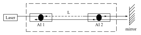
Figure 1: Schematic diagram of a gravitational wave detector using atomic interferometers as local inertial sensors

Now, we will describe the configuration in Fig.1 using the sensitivity function, and explain why some kinds of noise such as vibrational noise will be suppressed, but without affecting the signal arising from a gravitational wave. The sensitivity function is suggested firstly by Dick gjd87 ; sac98 , and then investigated in detail by others ccl08 ; gms08 ; bgb13 ; bzz13 with a time-domain atomic interferometer kc91 , which quantifies the influence of a relative laser phase shift $\delta\phi$ occurring at a time $t$ during the interferometer sequences on the transition probability $\delta P\left(\delta\phi,t\right)$; it is then defined in Ref. gjd87 ; sac98 as

$$g\left(t\right)=2\ast\underset{\delta\phi\rightarrow 0}{\lim}\frac{\delta P\left(\delta\phi,t\right)}{\delta\phi}.$$ (1)

If the time origin is chosen at the middle of the second Raman pulse, the sensitivity function $g\left(t\right)$ is an odd function. For the three pulses $\frac{\pi}{2}-\pi-\frac{\pi}{2}$ with durations respectively $\tau-2\tau-\tau$, we choose the initial time $t_{i}=-T$ and the final time $t_{f}=T$ to obtain the expression of the sensitivity function of the left interferometer as ccl08 ; gms08

$$g_{1}(t)=\left\{\begin{array}[c]{c}\sin(\Omega(T+t))\ \ \ ,-T\leqslant t<-T+\tau\\ \ 1\ \ \ \ \ \ \ \ \ \ \ \ \ ,-T\ +\tau\leqslant t<-\tau\\ -\sin\Omega t\ \ \ \ \ \ \ \ ,-\tau\leqslant t<\tau\\ -1\ \ \ \ \ \ \ \ \ \ \ \ ,\tau\leqslant t<T-\tau\\ -\sin\Omega(T-t)\ \ \ \ ,T-\tau\leqslant t\leqslant T\end{array}\right.$$ (2)

where $\Omega$ is the effective Rabi frequency, $T$ is the interrogation time between the two sequential pulses, and $g_{1}(t)=0$ for $\left|t\right|>T$ due to the phase jump occurring outside the interferometer.

According to the configuration in Fig.1, the interferometer on the right is operated with the same reflected laser pulse as the one on the left, and so the interference time is earlier on the time axis than that for the left one, so its sensitivity function is expressed as,

$$g_{2}(t)=\left\{\begin{array}[c]{c}\sin(\Omega(T+t+L))\ \ \ ,-T-L\leqslant t<-T+\tau-L\\ \ 1\ \ \ \ \ \ \ \ \ \ \ \ \ ,-T+\tau-L\leqslant t<-\tau-L\\ -\sin\Omega\left(t+L\right)\ \ \ \ \ \ \ \ ,-\tau-L\leqslant t<\tau-L\\ -1\ \ \ \ \ \ \ \ \ \ \ \ ,\tau-L\leqslant t<T-\tau-L\\ -\sin\Omega(T-t+L)\ \ \ \ ,T-\tau-L\leqslant t\leqslant T-L\end{array}\right.$$ (3)

where we have taken the speed of light $c=1$. Note that the function $g_{2}(t)$ is not odd in this situation. Then, the sensitivity function of differential measurement configurations at a specific time $t$ can be found as $g_{W}(t)=g_{2}(t)-g_{1}(t)$. After Fourier transformation, the transfer function is obtained as,

$$H(\omega) =\omega\int e^{-i\omega t}g_{W}(t)dt$$

$$=\frac{4\Omega\sin\frac{\omega T}{2}\left(\omega\cos\frac{\omega T}{2}+\Omega\sin\frac{\omega\left(T-2\tau\right)}{2}\right)}{\omega^{2}-\Omega^{2}}\left[\sin\omega L+i\left(1-\cos\omega L\right)\right]$$ (4)

where the first term is the transfer function of a single atomic interferometer ccl08 ; gms08 and the second term is related to the time delay of the light pulse. Note that the sensitivity function is calculated at the same time for the two interferometers, which means the pulses used to manipulate the two interferometers is independent. Thus the laser intensity noise would make the Rabi frequencies different for the two interferometers, meaning that $\Omega_{1}\neq\Omega_{2}$. According to the present laser power stabilisation technology kwd11 and previous noise analyses gms08 ; pcc01 for atomic interferometers, the laser intensity noise is sufficiently small that it can be neglected. Therefore, in this paper we ignore the influence of laser intensity noise on the expression of the sensitivity function.

As a consistency check, we can recreate Figure 6 of Ref. dgr08 with the same parameters by using our transfer function in Eq. (4). On the other hand, the sensitivity functions in Eqs. (2) and (3) do not indicate any differences between manipulations using two Raman pulses and using a single pulse yt11 ; ghkr13 , so we expect the differential measurement for the one-laser configuration to give a zero result, achieved by considering a common laser pulse to manipulate the two interferometers; in other words, the configurational sensitivity function should be zero for such a measurement. Assume that $\varphi$ is a phase change caused by vibration noise, and we have the differential expression for the same laser beams, $\Delta\varphi=\int\left(g_{1}(t)\frac{d\varphi\left(t\right)}{dt}-g_{2}(t)\frac{d\varphi\left(t-L\right)}{dt}\right)dt=\int\left(g_{1}(t+L)-g_{2}(t)\right)\frac{d\varphi\left(t\right)}{dt}dt=0$, as expected in Ref. yt11 . However, for the configuration described in Fig.1, if such cancellation is considered for the same reflected laser pulses, there will not be the same cancellation for the incoming ones, and vice versa, as discussed for AGIS in Ref. dgr08 . The model constructed here can illustrate this effect if we choose the time delay properly: the transfer function in Eq. (4) is chosen for the configuration in Fig.1 or AGIS, and $H^{{}^{\prime}}(\omega)=\omega\int\left(g_{1}(t+L)-g_{2}(t)\right)e^{-i\omega t}dt$ is chosen for the one-laser configuration, but note that $H^{{}^{\prime}}(\omega)$ would not be zero if the relative motion of the two interferometers is considered ghkr13 .

In order to present the advantage of this configuration, we take the vibration noise (see Ref. hsa13 for a detailed analysis of vibration noise) as an example and observe how much the noise is suppressed in the differential measurement. Assuming that the noise is brought into the detection device through coupling to the mirror or the laser platform, the influence of vibration noise on the total phase can be estimated by the variance in phase fluctuation ccl08 ; gms08 ,

$$\sigma_{\varphi}^{2}=\int_{0}^{\infty}\left|H_{\varphi}(\omega)\right|^{2}S_{\varphi}(\omega)d\omega=\frac{k^{2}}{\omega^{4}}\int_{0}^{\infty}\left|H_{\varphi}(\omega)\right|^{2}S_{a}(\omega)d\omega$$ (5)

where $k$ is the effective laser-field wavevector. Fig.2 is a vibration spectrum measured in our lab, without any isolation system added in the measurement process. With this vibration spectrum, we can estimate the influence of vibration noise on the final phase difference. For example, with the parameters $T=1.4$ s, $\tau=4\times 10^{-5}$ s, $k=1\times 10^{7}$ m^-1, $L=1000$ m, the differential value of the final phase shift is approximately $1.2\times 10^{-5}$ rad, which is significantly suppressed compared with the result obtained from a single interferometer, that is approximately $2.94$ rad.

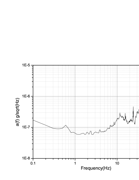
Figure 2: The spectrum of the vibration measured in our lab using a seismometer, without any isolation system included in the measurement process. a(f) is the acceleration noise power spectral density.

However, the signal from gravitational waves is not obtained directly from the result by the differential measurement. The signal can simply be obtained through two steps: firstly the gravitational wave induces phase fluctuations of light propagating along the baseline $L$ of our experimental setup, and secondly, the phase fluctuations are transferred into the atoms through our constructed configuration. Assuming that the gravitational wave is propagating along the direction perpendicular to the baseline $L$, and choosing coordinates carefully, for example, we choose the propagating direction of gravitational wave to be along the Z direction, and the baseline is along the X direction (see Ref. ew75 for the details). Thus the influence on the laser phase of gravitational waves travelling through the proposed detector is expressed as

$$\frac{1}{k}\frac{d\phi_{G}\left(t\right)}{dt}=\frac{1}{2}\left[h_{+}\left(t-L\right)-h_{+}\left(t\right)\right]$$ (6)

where the gravitational wave presents only the “+” polarisation in the transverse-traceless gauge. Without loss of generality, we take $h_{+}\left(t\right)=h\sin\left(\upsilon\left(t+\frac{L}{2}\right)+\phi_{0}\right)$ where $h$ is the amplitude of the gravitational waves, and $\phi_{0}$ is an arbitrary initial phase. Then, using the sensitivity function for the right interferometer, we obtain the phase shift from the signal of gravitational wave as

$$\Delta\phi_{G} =\int g_{2}(t)\frac{d\phi_{G}\left(t\right)}{dt}dt$$

$$\simeq 2\frac{hk}{\nu}\sin^{2}\left(\frac{\upsilon T}{2}\right)\sin\left(\frac{\upsilon L}{2}\right)\sin\left(\frac{\upsilon L}{2}+\upsilon T+\phi_{0}\right)$$ (7)

which is the same as the result obtained in Ref. dgr08 since the effective wavevector $k=k_{2}-k_{1}\simeq 2k_{2}$.

Thus from Eqs. (5) and (7), it is easy to see that a class of common noises is significantly suppressed, but the signal is not reduced by the differential measurement since it is detected only by the right interferometer, which included an implicit assumption that the distance between the laser and the left interferometer is much less than $L$.

III Sensitivity constrained by noise

In the last section, we use the sensitivity function to analyse the configuration described in Fig.1, and in this section we investigate how different kinds of noise influence the sensitivity of such a configuration. In particular, we compare the difference in sensitivities constrained by shot noise with that arising from the phase noise which is caused by vibrations and laser frequency instability. The vibration spectrum, as an example, is shown in Fig.2 and the laser frequency spectrum is shown in Fig.3, both of which are experimentally obtained in our lab. In what follows, we will calculate these sensitivities and get their corresponding curves.

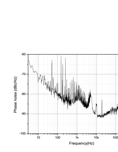
Figure 3: The spectrum of the laser frequency in our lab

In the AGIS scheme, the large-momentum-transfer (LMT) beam splitters that consist of a $\frac{\pi}{2}$ pulse and $N$ pairs of $\pi$ pulses and the LMT mirror that included $2N+1$ $\pi$ pulses in the sequence are used to manipulate the atomic interferometers with a Bragg process mcc07 ; ckk11 . Without affecting our purpose in this paper, we chose $N=1$. Therefore, the sensitivity function of the left interferometer is expressed as

$$g_{1}(t)=\left\{\begin{array}[c]{c}\sin\Omega(t+T)\ \ \ \ \ \ \ \ \ \ \ \ \ \ -T\leqslant t<-T+\tau\\ \ \ \ \ \ \ \ \ \ 1\ \ \ \ \ \ \ \ \ \ \ \ \ \ \ \ \ \ \ -T+\tau\leqslant t<-T+3\tau\\ \frac{1}{2}[3-\cos\Omega(T+t-3\tau)]\ \ \ \ \ \ -T+3\tau\leqslant t<-T+5\tau\\ \ \ \ \ \ \ 2\ \ \ \ \ \ \ \ \ \ \ \ \ \ \ \ \ \ \ -T+5\tau\leqslant t<-5\tau\\ \frac{1}{2}[3+\cos\Omega(t+5\tau)]\ \ \ \ \ \ \ \ \ -5\tau\leqslant t<-3\tau\\ \ 1\ \ \ \ \ \ \ \ \ \ \ \ \ \ \ \ \ \ \ -3\tau\leqslant t<-\tau\\ \ -\sin\Omega t\ \ \ \ \ \ \ \ \ \ \ \ \ \ \ \ -\tau\leqslant t<0\end{array}\right.$$ (8)

written for the time period of $t<0$ since we can obtain an odd function when we choose the time origin to be at the middle of the middle $\pi$ pulse. From the last section, we know that $g_{2}(t)=g_{1}(t+L)$ without considering the relative motion of the two interferometers. Thus the differential sensitivity function $g_{W}(t)=g_{2}(t)-g_{1}(t)$ and its transfer function is obtained through the same formula $H(\omega)=\omega\int e^{-i\omega t}g_{W}(t)dt$. We have also checked the transfer function by comparing it with Figure 6 of Ref. dgr08 , generating the figure with the same parameters as those used in the paper, and the nearly unchanged result shows that the introduction of LMT does not influence the passband of the device which is truncated at the frequency of $\frac{1}{L}$ and the Rabi frequency $\Omega$.

As shown in Ref. dgr08 , the noise will not be amplified, since all but the beginning and end of each LMT pulse will be common to the two interferometers, if the Rabi frequency $\Omega$ and the distance $L$ between the two interferometers were chosen properly. That means that the manipulation using LMT pulses will increase the measurement sensitivity in a way proportional to $N$. In general, the sensitivity of gravitational wave detection can be obtained by the equation,

$$SNR=\frac{\Delta\phi_{G}}{\sigma_{\varphi}}$$ (9)

which is the ratio of signal to noise, and the signal $\Delta\phi_{G}$ has included the result of LMT. In Ref. dgr08 , the detection sensitivity constrained by shot noise for some range of frequencies was better for a larger distance $L$, but the frequency range was found to be dependent on the distance $L$. In other words, when the distance between the two interferometers varies, the corresponding optimal detection frequencies will also vary, which is the requirement of the approximation taken in Ref. dgr08 . In this paper, we do not take such approximation for the leading term of the calculated result, as seen in the expression of Eq. (7). Our result was presented in Fig.4, and a comparison of two separation distances indicates that a larger separation distance could improve the sensitivity, which is shown clearly in the next section. In particular, according to our estimation for shot noise, the distance has to be as large as $10^{8}$ m if the amplitude of gravitational wave is of the order of $h\sim 10^{-20}$.

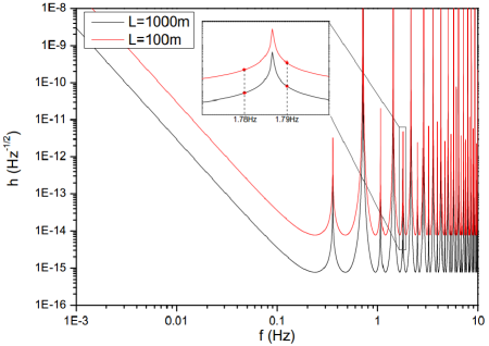
Figure 4: The sensitivity curve to gravitational wave of frequency f, limited by shot noise. The different parameters are labeled in the diagram. The common parameters that were used: $\tau=4\times 10^{-5}$s, $k=1\times 10^{7}$m^-1. These are similar to the proposal in the terrestrial experiment of Ref. dgr08 .

The sensitivity curves related to the vibration noise and laser frequency noise have not been investigated before, and here we also plot these values in Fig.5. Surprisingly, the sensitivity is nearly unchanged when the distance between the two interferometers is increased. This is consistent with the analysis for the vibration noise in Ref. bt12 , where the ratio of signal to vibration noise is independent on the distance between two interferometers, under the approximation of $\omega L\ll 1$. But for the single-arm light interferometer, this ratio is proportional to $1/L^{2}$ bt12 , so it is necessary to investigate further the influence of the distance between two interferometers.

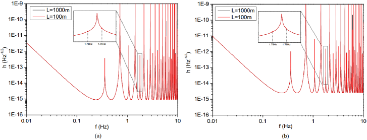
Figure 5: The sensitivity curve to gravitational wave of frequency f, limited by vibration noise (a) and laser frequency noise (b). The parameters are same as that in Fig.4.

IV Influence of the distance between two interferometers

In gravitational wave detection, the relation of sensitivity with the measurable frequencies plays an important role for the estimation of the detection scheme. From the last section, we notice that sensitivity curves almost look the same for the shot noise, vibration noise, and laser-frequency noise, and an obvious difference is the change in sensitivity when the distance between two interferometers changes. In this section, we study this relation in detail without any approximation for the leading term, and present the difference of influence on gravitational wave detection arising from vibration noise or laser frequency noise from that arising from shot noise.

For the shot noise, the sensitivity will be better for a larger distance $L$, which is confirmed by studying the relation of measurable amplitude of gravitational wave with the distance $L$, as in Fig.6a. It was noticed that the sensitivity curves is different for the two chosen frequencies $f=1.78$ Hz and $f=1.79$ Hz (they are labeled in Fig.4 with two different red points) at any given distance $L$, but the changing trends are the same for two curves. Actually, for the shot noise, the changing trend is the same for any given frequency, although the sensitivity is different at some given distance $L$. Moreover, the sensitivity presented here seemed worse than what would be required for gravitational wave detection, because the parameter $k$ was chosen to be a value smaller than that in Ref. dgr08 . It is easy to see that if we take the parameter $k$ with the same value with that in Ref. dgr08 , the sensitivity will nearly reach $10^{-17}$ at the distance $L=1000$m. In particular, $k$ is considered as a free parameter due to LMT, and doesn’t have to be directly tied to the choice of atom and transitions. Here the important thing is to understand the relation of sensitivity with the separation distance between two interferometers, and in what follows we give a different form of this relation when the vibration noise and laser-frequency noise are considered.

Figure 6: The relation of sensitivity with the distance $L$ between two interferometers, limited by shot noise (a), vibration noise (b), and laser frequency noise (c). The common parameters are still used: $\tau=4\times 10^{-5}$s, $k=1\times 10^{7}$m^-1. The different frequency parameters are labeled in the diagram, which are corresponding to the points labeled in Fig.4 and Fig.5.

As stated in the last section, the vibration noise arises from the laser platform or the mirror and coupled into the final results with different proportions for different frequencies, as seen from the transfer function (4). Then we take $\sigma_{\phi}$ in Eq. (9) as the perturbation of vibration noise to determine the sensitivity. From Fig.6b, it can be seen that the changing trend of the sensitivity with the separation distance between two interferometers is different for the two chosen frequencies $f=1.78$ Hz and $f=1.79$ Hz. Actually, for every frequency in sensitivity curves of Fig.5, the changing trend of the sensitivity with the separation distance have the same lineshape with either that of frequencies $f=1.78$ Hz or that of frequencies $f=1.79$ Hz. This is subtly different from the result obtained in Ref. bt12 but is not in conflict with each other, since the change in Fig.6b is small. However, the result presented in Fig.6b shows that a larger distance does not improve the sensitivity, which is related to noise. Our result is also applicable to other common noises such as laser phase noise etc., which is easy to understand since the influence of vibration on the final result is similar to the influence from phase noises mjv06 . It was noted that the sensitivity is far from what is required for gravitational wave detection, since the vibration spectrum in Fig.2 is measured without using any vibration-isolation system in the measurement process, and we have given a rough estimate for its amplitude in the second section. Moreover, the different values of sensitivity for two different frequencies can be explained with reference to the case of shot noise. However, the distinctly different behaviours in relation to separation distance between Fig. 6b and Fig. 6a shows that vibration noise influences the final measurement result with a quite different way from shot noise.

From Fig.6c, we see that the result derived from the laser frequency noise, which also contributes to the laser phase noise, is almost the same as that from the vibration noise. Laser frequency noise is a dominant background noise for gravitational wave detection using light interferometers, and it could be suppressed by applying single laser pulse to operate the two atomic interferometers simultaneously yt11 ; ghkr13 although there is still some technological difficulties with this kind of measuring scheme plb14 . For our scheme under consideration in Fig.1, although the reflected laser pulse is the same for the two interferometers, the incoming ones are different, which is main source of laser frequency noise. Here, to compare the behaviour of the laser frequency noise influencing the detection configuration shown in Fig.1 with other types noise, we use the laser frequency spectrum in Fig.3, like the vibration spectrum, without using any methods to suppress the laser frequency noise. It is noted that the sensitivity varies slightly with the distance between two interferometers, although the phase change caused by laser frequency noise will increase linearly when the distance is lengthened, which is approximately estimated by an approximate estimation as $\delta k\cdot L$ where $\delta k$ is due to the average deviation of the laser frequency over the finite time length of the pulse. This amplification will nearly cancel the increase in the signal from gravitational waves, and thus leads to the resulting slight change in sensitivity.

Actually the most significant estimation for practical observations lies in the whole average noise, that is $\sigma_{\Delta\varphi}=\sqrt{\sigma_{\phi_{i}}^{2}+\sigma_{\phi_{j}}^{2}+\sigma_{0}^{2}}$ where $\sigma_{0}^{2}$ is from shot noise, $\sigma_{\phi_{i}}^{2}$ are from known noise sources such as phase noise etc., and $\sigma_{\phi_{j}}^{2}$ are from potential systematic effects such as some environmental effects. According to the level of noise, given here by shot noise and vibration noise, the sensitivity limited by their average noise may still be improved by a large distance $L$, but this improvement is dependent on which type of noise is dominant in the observation, for example, in the 1999 experiment to measure gravitational acceleration by dropping atoms, the phase noise is about a hundred times larger than atomic shot noise pcc99 ; zcz13 . Thus, if phase noise is dominant in the future gravitational wave observation, whether the separation distance between two interferometers should be made larger has to be considered carefully. That is to say, a more economic selection for the distance $L$ may be possible, dependent on the actual level of noise.

In particular, we pointed out that although our analysis was carried out using the parameters $T=1.4$ s, $\tau=4\times 10^{-5}$ s, $k=1\times 10^{7}$ m^-1 which will determine the passband of the single-arm scheme of gravitational wave detectors, the conclusion will not change if we take other physically allowed values for these parameters. Moreover, $L$ is also an factor that can determine the passband, but from Fig. 6b and 6c, we find that our conclusions are not influenced by the positions of the passband. On the other hand, although our analysis is for the ground-based single-arm scheme of gravitational wave detection, it is still meaningful and significant for the similar space-based scheme, and in particular, for the space-based situation, the vibration noise is stronger ac04 ; zfc12 and the laser frequency noise might be more difficult to be overcome. If the spectra for measuring vibration or laser frequency instability for a space-based situation was used to do the same calculation with that for ground-based ones, the corresponding results can also be obtained, and in our view it is highly possible to arrive at the same conclusions as presented in Fig.6.

V Conclusion

In this paper, we have described the sensitivity function for single-arm gravitational wave detector based on atomic interferometers, in which we explain the way that a range of noise from different sources, such as vibration noise and laser frequency noise, can enter the detector, but in a different way from that the signal arising from gravitational waves enters the detector. We have also studied the relation of the measurement sensitivity with the distance between two interferometers, and showed that the sensitivity limited by these common sources of noise will nearly be unchanged when the distance is greatly increased, which is significantly different from the case for shot noise. Then a next significant thing is to investigate the sensitivity which is limited by other kinds of noise, in particular, by the Newtonian gravity background which might influence the sensitivity with a different way, as the gravity background fluctuates in value depending on position and time.

- (1) J. R. Gair, M. Vallisneri, S. L. Larson, and J. G. Baker, Living Rev. Relativity 16, 7 (2013).
- (2) B. Abbott et al. (LIGO Scientific Collaboration), Rep. Prog. Phys. 72, 076901 (2009).
- (3) T. Accadia et al. (VIRGO Scientific Collaboration), J. Instrum. 7, P03012 (2012).
- (4) S. Dimopoulos, P. W. Graham, J. M. Hogan, M. A. Kasevich, and S. Rajendran, Phys. Rev. D 78, 122002 (2008).
- (5) S. Dimopoulos, P. W. Graham, J. M. Hogan, M. A. Kasevich, and S. Rajendran, Phys. Lett. B 678, 37 (2009).
- (6) P. L. Bender, Phys. Rev. D 84, 028101 (2011).
- (7) S. Dimopoulos, P. W. Graham, J. M. Hogan, M. A. Kasevich, and S. Rajendran, Phys. Rev. D 84, 028102 (2011).
- (8) J. M. Hogan, D. M. S. Johnson, S. Dickerson, et al. Gen. Relativ. Gravit. 43, 1953 (2011).
- (9) P. L. Bender, Gen. Relativ. Gravit. 44, 711 (2012).
- (10) N. Yu, and M. Tinto, Gen. Relativ. Gravit. 43, 1943 (2011).
- (11) P. W. Graham, J. M. Hogan, M. A. Kasevich, and S. Rajendran, Phys. Rev. Lett. 110, 171102 (2013).
- (12) P. L. Bender, Phys. Rev. D 89, 062004 (2014).
- (13) R. X. Adhikari, Rev. Mod. Phys. 86, 121 (2014).
- (14) Lin Zhou, Shitong Long, Biao Tang, et al, Phys. Rev. Lett. 115, 013004 (2015).
- (15) M. J. Snadden, J. M. McGuirk, P. Bouyer, K. G. Haritos, and M. A. Kasevich, Phys. Rev. Lett. 81, 971 (1998).
- (16) J. G. Baker and J. I. Thorpe, Phys. Rev. Lett. 108, 211101 (2012).
- (17) G. J. Dick, Local Osillator induced instabilities, in Proc. Nineteenth Annual Precise Time and Time interval, 133-147 (1987).
- (18) G. Santarelli, C. Audoin, A. Makdissi, P. Laurent, G.J. Dick, A. Clairon, IEEE Trans. on Ultr., Ferr. and Freq. Contr. 45, 887 (1998).
- (19) P. Cheinet, B. Canuel, F. P. D. Santos, A. Gauguet, F. Leduc, and A. Landragin, IEEE Trans. on Instrum. Mess. 57, 1141 (2008).
- (20) J. L. E. Gouët, et al. Appl. Phys. B 92, 133 (2008).
- (21) B. Barrett, P.-A. Gominet, E. Cantin, L. Antoni-Micollier, A. Bertoldi, B. Battelier and P. Bouyer, arXiv: 1311.7033.
- (22) B. Tang, B. Zhang, L. Zhou, J. Wang, and M. S. Zhan, Research in Astronomy and Astrophysics 15, 333-347 (2015).
- (23) M. A. Kasevich and S. Chu, Phys. Rev. Lett. 67, 181 (1991).
- (24) P. Kwee, B. Willke, and K. Danzmann, Appl. Phys. B 102, 515 (2011).
- (25) A. Peters, K. Y. Chung and S. Chu, Metrologia 38, 25 (2001).
- (26) J. Harms, B. J. J. Slagmolen, R. X. Adhikari, et al, Phys. Rev. D 88, 122003 (2013).
- (27) F. B. Estabrook and H. D. Wahlquist, Gen. Relativ. Gravit. 5, 439 (1975).
- (28) H. Muller, S. W. Chiow, Q. Long, S. Herrmann, and S. Chu, Phys. Rev. Lett. 100, 180405 (2008).
- (29) S.-w. Chiow, T. Kovachy, H.-C. Chien, and M. A. Kasevich, Phys. Rev. Lett. 107, 130403 (2011).
- (30) A. Miffre, M. Jacquey, M. Büchner, G. Trénec, and J. Vigué, Appl. Phys. B 84, 617 (2006).
- (31) A. Peters, K. Y. Chung and S. Chu, Nature 400, 849 (1999).
- (32) B. Zhang, Q. Y. Cai, and M. S. Zhan, EPJD 67, 184 (2013).
- (33) B. N. Agrawal and H.-J. Chen, Smart Mater. Struct. 13, 873–880 (2004).
- (34) Y. Zhang, B. Fang and Y. Chen, Meccanica 47, 1185–1195 (2012).