Integer Low Rank Approximation of Integer matrices

Abstract

Integer data sets frequently appear in many applications in sciences and technology. To analyze these, integer low rank approximation has received much attention due to its capacity of representing the results in integers preserving the meaning of the original data sets. To our knowledge, none of previously proposed techniques developed for real numbers can be successfully applied, since integers are discrete in nature. In this work, we start with a thorough review of algorithms for solving integer least squares problems, and then develop a block coordinate descent method based on the integer least squares estimation to obtain the integer low rank approximation of integer matrices. The numerical application on association analysis and numerical experiments on random integer matrices are presented. Our computed results seem to suggest that our method can find a more accurate solution than other existing methods for continuous data sets.

1 Introduction

The study of integer approximation has long been a subject of interest in many areas such as networks of communication, data organization, environmental chemistry, lattice design, and finance [1, 2, 3, 4]. In this work, we consider integer low rank approximation of integer matrices (ILA). Let $\mathbb{Z}^{m\times n}$ denote the set of $m\times n$ integer matrices. Then, the ILA problem can be stated as follows:

(ILA) Given an integer matrix $A\in\mathbb{Z}^{m\times n}$ and a positive integer $k<\min\{m,n\}$, find $U\in\mathbb{Z}^{m\times k}$ and $V\in\mathbb{Z}^{k\times n}$ so that the residual function

$$~{}f(U,V):=\|A-UV\|_{F}^{2}$$ (1)

is minimized.

Concretely, the ILA is to represent an original integer data set in a space spanned by integer basis vectors using integer representations minimizing the residual function in (1). One example that characterizes this problem is the so-called market basket transactions. See Table 1 for example, where it shows orders from five customers $C_{1},\ldots,C_{5}$.

Table 1: An integer representation of the transaction example

	Bread	Milk	Diapers	Eggs	Chips	Beer
$C_{1}$	2	1	3	0	2	5
$C_{2}$	2	1	1	0	2	4
$C_{3}$	0	0	4	2	0	2
$C_{4}$	4	2	2	0	4	8
$C_{5}$	0	0	2	1	0	1

This should be a huge data set with many customers and shopping items in practice. Similar to the discussion given in [5, 6], we would like to discover an association rule such as “$\mbox{\{2 diapers, 1 egg\}}\Rightarrow\mbox{\{1 beer\}}$”, which means that if a customer has shopped for two diapers and one egg, he/she has a higher possibility of shopping for one beer. The “possibility” is determined by a weight associated with each transaction. To keep the number of items to be integer, the weight is defined by nonnegative integers corresponding to the representative transaction. For example, we can approximate the original integer data set, which is define in Table 1, by two representative transactions ${[2,1,1,0,2,4]}$ and ${[0,0,2,1,0,1]}$ with the weight determined by a $5\times 2$ integer matrix, that is,

$$A=\left[\begin{array}[]{cccccc}2&1&3&0&2&5\\ 2&1&1&0&2&4\\ 0&0&4&2&0&2\\ 4&2&2&0&4&8\\ 0&0&2&1&0&1\\ \end{array}\right]\approx\left[\begin{array}[]{cc}1&1\\ 1&0\\ 0&2\\ 2&0\\ 0&1\\ \end{array}\right]\left[\begin{array}[]{cccccc}2&1&1&0&2&4\\ 0&0&2&1&0&1\\ \end{array}\right].$$ (2)

This is indeed a rank-two approximation which provides the possible shopping behaviors of the original five customers.

Note that the study of the ILA is to analyze original integer (i.e.,discrete) data in term of integer representatives so that the underlying information can be conveyed directly. Due to the discrete characteristic, conventional techniques such as SVD [7] and the nonnegative matrix factorization (NMF) [8, 9, 10, 11, 12, 13] are inappropriate and unable to solve this problem. Also, we can regard this problem as a generalization of the so-called Boolean matrix approximation, where entries of $A$, $U$ and $V$ are limited to $\mathbb{Z}_{2}:=\{0,1\}$, i.e., binaries, and columns of the matrix $U$ are orthogonal. In [5, 6], Koyutürk et al. [5, 6] proposed a nonorthogonal binary decomposition approach to recursively approximate the given data by the rank-one approximation. This idea is then generalized in [4] to handle integer data sets, called the binary-integer low rank approximation (BILA), and can be defined as follows:

(BILA) Given an integer matrix $A\in\mathbb{Z}^{m\times n}$ and a positive integer $k<\min\{m,n\}$, find $U\in\mathbb{Z}_{2}^{m\times k}$ satisfying $U^{\top}U=I_{k}$, where $I_{k}$ is a $k\times k$ identity matrix, and $V\in\mathbb{Z}^{k\times n}$ such that the residual function

$$f(U,V):=\|A-UV\|_{F}^{2}$$

is minimized.

To demonstrate the BILA, we use the scenario of selling laptops. We know that each laptop includes $n$ slots which can be equipped with only one type of specified options, for example, 8GB memory or 1TB hard drive. Here, the uniqueness is determined by the orthogonal columns of $U$. Let $t_{i}$ represent the number of different types of options for each slot. This implies that we have $\prod_{i=1}^{n}t_{i}$ possible cases. To efficiently fulfill different customer orders and increase the sales, the manager needs to decide a few basic models, e.g., $k$ basic ones. One plausible approach is to learn the information from past experience. This amounts to first labeling every possible option in a slot by an integer while each integer is corresponding to a particular attribute. For example, record $m$ past customers’ orders into an $m\times n$ integer data matrix. Second, divide the orders into $k$ different integer clusters. These $k$ clusters then lead to the $k$ different models that should be provided; see also [3] for a similar discussion in telecommunications industry.

Besides, the BILA behaves like the $k$-means problem. That is because all rows of $A$ are now divided into $k$ disjoint clusters due to the fact that $U=[u_{ij}]\in\mathbb{Z}_{2}^{m\times k}$ and $U^{\top}U=I_{k}$, and each centroid is the rounding of the means of the rows from each disjoint cluster [4]. It is known that the $k$-means problem is NP-hard [14, 15]. This might indicate the possibility of solving the BILA is NP-hard. Moreover, it is true that the BILA is a special case of ILA. We thus conjecture that the ILA is an NP-hard problem.

To handle this “seemingly” NP-hard problem, we thus organize this paper as follows. In Section 2, we investigate the ILA in terms of the block coordinate descent (BCD) method and discuss some characteristics related to orthogonal constraints. In Section 3, we review the methods for solving integer least squares problem, apply them to solve the ILA, and present a convergence theorem correspondingly. Three examples are demonstrated in Section 4 to show the capacity and efficiency of our ILA approaches and the concluding remarks are given in Section 5.

2 Block Coordinate Descent

The framework of the BCD method includes the following procedures:

1. Provide an initial value $V\in\mathbb{Z}^{k\times n}$.

2. Iteratively, solve the following problems until a stopping criterion is satisfied:

   $$\min_{U\in\mathbb{Z}^{m\times k}}\|A-UV\|_{F}^{2},$$ (3a)

   $$\min_{V\in\mathbb{Z}^{k\times n}}\|A-UV\|_{F}^{2}.$$ (3b)

Alternatively, we can initialize $U$ first and iterate (3a) and  (3b) in the reverse order. Note that in Step 2, each subproblem is required to find the optimal matrices $U$ or $V$ so that $\|A-UV\|_{F}$ is minimized. Observe further that

$$\|A-UV\|_{F}^{2}=\sum_{i}\|A(i,:)-U(i,:)V\|_{2}^{2}=\sum_{j}\|A(:,j)-UV(:,j)\|_{2}^{2}.$$ (4)

It follows that (4) is minimized, if for each $i$,

$$\|A(i,:)-U(i,:)V\|_{2}$$

is minimized and for each $j$,

$$\|A(:,j)-UV(:,j)\|_{2}$$

is minimized. Let the symbol “round(X)” denote a function which rounds each element of $X$ to the nearest integer. Since the 2-norm is invariant under orthogonal transformations, one immediate result can be stated as follows.

Theorem 1.

Suppose $\mathbf{a}\in\mathbb{Z}^{1\times n}$ and $V\in\mathbb{Z}^{k\times n}$ with $n\geq k$ and $VV^{\top}=I_{k}$, where $I_{k}$ is a $k\times k$ identity matrix. Let

$$\hat{\mathbf{u}}=\rm{round}(\mathbf{a}V^{\top})\in\mathbb{Z}^{1\times k}.$$ (5)

Then the following is true:

$$\|\mathbf{a}-\hat{\mathbf{u}}V\|_{2}\leq\min_{\mathbf{u}\in\mathbb{Z}^{1\times k}}\|\mathbf{a}-\mathbf{u}V\|_{2}.$$

With an obvious change of notation, an analogous statement would be true for $\mathbf{a}\in\mathbb{Z}^{m\times 1}$, and $U\in\mathbb{Z}^{m\times k}$ having $m\geq k$ and $U^{\top}U=I_{k}$. Besides, Theorem 1 provides a way to obtain the optimal matrix $U$ in the following way, whose proof is by direct observation.

Theorem 2.

Suppose $A\in\mathbb{Z}^{m\times n}$ and $V\in\mathbb{Z}^{k\times n}$ with $n\geq k$ and $VV^{\top}=I_{k}$. Let

$$\widehat{U}=\rm{round}(AV^{\top})\in\mathbb{Z}^{m\times k}.$$

Then the following is true:

$$\|A-\widehat{U}V\|_{F}\leq\min_{U\in\mathbb{Z}^{m\times k}}\|A-UV\|_{F}.$$

Similarly, the optimal matrix $V$ can be obtained immediately, provided that $U$ is given and $U^{\top}U=I_{k}$. But, could the optimal matrices $U$ and $V$ be obtained simply by rounding real optimal solutions $({A}V^{\top})(VV^{\top})^{-1}$ and $(U^{\top}U)^{-1}(U^{\top}{A})$, respectively? Definitely, the answer is no due to the discrete property embedded in the integer matrix.

Example 1.

Consider $\min_{\mathbf{v}\in\mathbb{Z}^{k\times 1}}\|\mathbf{a}-U\mathbf{v}\|_{2}$, where $U=\left[\begin{array}[]{cc}8&1\\ 9&2\end{array}\right]$ and $\mathbf{a}=\left[\begin{array}[]{c}16\\ 17\end{array}\right]$. The optimal solution $\mathbf{v}_{\mbox{opt}}\in\mathbb{R}^{2\times 1}$ can be obtained by computing

$$\mathbf{v}_{\mbox{opt}}=(U^{\top}U)^{-1}(U^{\top}\mathbf{a})\approx\left[\begin{array}[]{c}2.1429\\ -1.1429\end{array}\right].$$

Considering integer vectors $\mathbf{v}_{1}=\left[\begin{array}[]{c}2\\ -1\end{array}\right]$, $\mathbf{v}_{2}=\left[\begin{array}[]{c}2\\ -2\end{array}\right]$, $\mathbf{v}_{3}=\left[\begin{array}[]{c}3\\ -1\end{array}\right]$ and $\mathbf{v}_{4}=\left[\begin{array}[]{c}3\\ -2\end{array}\right]$ which are around $\mathbf{v}_{\mbox{opt}}$, we see that $\|\mathbf{a}-U\mathbf{v}_{i}\|_{2}=\sqrt{2},\sqrt{13},\sqrt{113},6\sqrt{2}$ for $i=1,\ldots,4$, respectively. However, if we take $\mathbf{v}=\left[\begin{array}[]{c}2\\ 0\end{array}\right]$, we have $\|\mathbf{a}-U\mathbf{v}\|_{2}=1<\|\mathbf{a}-U\mathbf{v}_{i}\|_{2}$ for $i=1,\ldots,4$. See also Figure 1 for a demonstration through the geometric viewpoint.

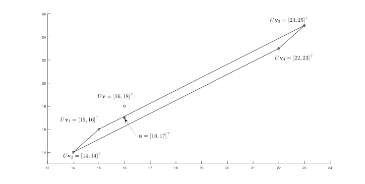
Fig. 1: A counterexample for the rounding approach

It follows that the major mechanism of the BCD method lies in computing the global minimum in each iteration. To this end, we discuss the integer least squares problem in the next section and apply it to solve the ILA column-by-column/row-by-row so that a sequence of descent residuals can be expected.

3 Integer Least Squares Problems

Given a vector $y\in\mathbb{R}^{m}$ and a matrix $H\in\mathbb{R}^{m\times n}$ with full column rank, the integer least squares (ILS) problem is defined as

$$\min_{\mathbf{x}\in\mathbb{Z}^{n}}\|\mathbf{y}-H\mathbf{x}\|_{2}^{2}.$$ (6)

Solving the ILS problem is known to be NP-hard [16]. In this section, we first review a common approach for solving ILS problems. This approach is referred to be the enumeration approach and usually relies on two major processes, reduction and search. Second, we consider the ILS problem with box constraints (ILSb), which can be defined as:

$$\min_{\mathbf{x}\in\mathcal{B}}\|\mathbf{y}-H\mathbf{x}\|_{2}^{2},$$ (7)

where $\mathcal{B}=\mathcal{B}_{1}\times\cdots\times\mathcal{B}_{n}$ with $\mathcal{B}_{i}=\{x_{i}\in\mathbb{Z}:\ell_{i}\leq x_{i}\leq u_{i}\}$. We then enhance this idea of solving the ILSb to solve the ILA with box constraints, where entries are subject to a bounded region. Third, we will discuss some convergence properties for the ILA.

3.1 ILS

Typical methods for solving ILS problems in the literature have two stages: reduction (or preprocessing) and search.

To do the reduction, the idea is based on the well-known process, Lenstra-Lenstra-Lovász [17] (LLL) reduction. This process is to transform the ILS problem defined in (6) into a reduced form

$$\min_{\mathbf{z}\in\mathbb{Z}^{n}}\|\hat{\mathbf{y}}-R\mathbf{z}\|_{2}^{2},$$ (8)

in terms of a specific QRZ factorization [18] such that

$$Q^{\top}HZ = \left[\begin{array}[]{c}R\\ 0\end{array}\right],\,\hat{\mathbf{y}}=Q_{1}^{\top}\mathbf{y},\,\mathbf{z}=Z^{-1}\mathbf{x},$$ (11)

where $Q=\left[\begin{array}[]{cc}Q_{1}&Q_{2}\end{array}\right]\in\mathbb{R}^{m\times m}$ is orthogonal, $Z\in\mathbb{Z}^{n\times n}$ is unimodular (i.e., $\det(Z)=\pm 1$), and $R=[r_{i,j}]\in\mathbb{R}^{n\times n}$ is an upper triangular matrix satisfying the following conditions:

$$|r_{i-1,j}| \leq \dfrac{|r_{i-1,i-1}|}{2},\quad 2\leq i<j\leq n,$$ (12a)

$$\delta r^{2}_{i-1,i-1} \leq r^{2}_{i-1,i}+r_{i,i}^{2},\quad 2\leq i\leq n,$$ (12b)

where $\delta$ is a parameter satisfying $\frac{1}{4}<\delta\leq 1$. In this work, we choose $\delta=1$ as suggested in [18]. Then it can be easily obtained from (12) that the diagonal entries of $R$ have the following properties:

$$|r_{i-1,i-1}|\leq\frac{2}{\sqrt{3}}|r_{i,i}|,\quad 2\leq i\leq n.$$

Once having these properties, the matrix $R$ can enhance the efficiency of a typical search algorithm for (8); see [1, 19] and Algorithm 1 for more details.

Input: A matrix $H\in\mathbb{R}^{m\times n}$ and a vector $y\in\mathbb{R}^{m}$.

Output: An upper triangular matrix $R\in\mathbb{R}^{n\times n}$, an unimodular matrix $Z\in\mathbb{Z}^{n\times n}$, and a vector $\hat{\mathbf{y}}\in\mathbb{R}^{n}$ for the computation of (8) and (11).

begin compute the QR decomposition of $H$, i.e.,

$H=\left[\begin{array}[]{cc}Q_{1}&Q_{2}\end{array}\right]\left[\begin{array}[]{c}R\\ 0\end{array}\right]$;

set $Z=I_{n}$, $\hat{\mathbf{y}}=Q_{1}^{\top}\mathbf{y}$ and $k=2$;

while $k\leq n$ do /*Size Reduction on $r_{1:k-1,k}$

for $i=k-1,\ldots,1$ do $R\leftarrow RZ_{i,k}$,  $Z\leftarrow ZZ_{i,k}$;

end if $r_{k-1,k-1}^{2}>(r_{k-1,k}^{2}+r_{k,k}^{2})$ then /* Permutation and Triangularization

$R\leftarrow G_{k-1,k}RP_{k-1,k}$,  $Z\leftarrow ZP_{k-1,k}$,  $\hat{\mathbf{y}}\leftarrow G_{k-1,k}\hat{\mathbf{y}}$;

if $k>2$ then $k\leftarrow k-1$;

end else $k\leftarrow k+1$;

end end end

Algorithm 1 (LLL reduction) [18] $[R,Z,\hat{\mathbf{y}}]=\textsc{LLL}(H,\mathbf{y})$

7

7

7

7

7

7

7

Note that the entire QRZ factorization includes a QR factorization and two types of transformations, integer Gauss transformations (IGTs) and permutations, to implicitly update $R$ right after the QR factorization of $H$ so that it satisfies (12). To make this work more self-contained, we briefly introduce the major results here; see [18] for more details.

First, the IGTs are done by an unimodular matrix $Z_{i,j}$ which is given by

$$Z_{i,j}=I_{n}-\zeta_{ij}e_{i}e_{j}^{\top},$$

where $i\neq j$ and $\zeta_{ij}=\rm{round}(\dfrac{r_{i,j}}{r_{i,i}})$. We then multiply $R$ with $Z_{i,j}$ ($i<j$) from the right and obtain an updated matrix

$$\widehat{R}\equiv RZ_{i,j}=R-\zeta_{i,j}Re_{i}e_{j}^{\top}.$$

It can be seen that entries of $\widehat{R}$ are equal to entries of $R$, except that $\hat{r}_{k,j}=r_{k,j}-\zeta_{i,j}r_{k,i}$ for $k=1,\ldots,i$, and satisfies (12a).

Second, if (12b) is not satisfied for some $i$, we then swap columns $i-1$ and $i$ of $R$ by a permutation matrix, denoted by $P_{i-1,i}$. But the resulting matrix $R$ is no longer upper triangular and is required to be trangularized. In [17], the Gram-Schmidt process (GP) is applied to bring back the structure. That is, find an orthogonal matrix $G_{i-1,i}$ so that the resulting matrix

$$\widehat{\widehat{R}}=G_{i-1,i}\widehat{R}P_{i-1,i}$$

is an upper triangular and satisfies (12a).

It should be noted that right after these transformations, two characteristics are worthy of our attention [20, 21]. First, it can be seen that

$$\min_{\hat{\mathbf{z}}\in\mathbb{Z}^{n}}\|\hat{\mathbf{y}}-\widehat{R}\hat{\mathbf{z}}\|_{2}^{2}=\min_{\mathbf{z}\in\mathbb{Z}^{n}}\|\hat{\mathbf{y}}-R\mathbf{z}\|_{2}^{2},$$

since $Z_{i,j}$ is unimodular, that is, the application of the IGT will not affect the optimal value of (8). Second, it follows from a direct computation that

$$\hat{\hat{r}}^{2}_{i-1,i-1} = \hat{r}_{i-1,i}^{2}+r_{i,i}^{2}<{r}_{i-1,i}^{2}+r_{i,i}^{2},$$

$$|\hat{\hat{r}}_{i-1,i-1}\hat{\hat{r}}_{i,i}| = |\det(\widehat{\widehat{R}})|=|\det(R)|=|r_{i-1,i-1}r_{i,i}|.$$

This implies that though the IGT will not reduce the optimal value of (8), it will reduce the absolute value of the original $(i-1,i-1)$ entry and enlarge the absolute value of the $(i,i)$ entry and hence make a typical search algorithm more efficient. However, the calculation of the IGTs would be time-consuming. For example, in Algorithm 1, we need to recompute the IGTs in previous step, once (12b) is not satisfied. To prevent from this calculation and enhance the efficiency of the algorithm, the IGTs are computed only when a permutation is required. This result can be seen in Algorithm 2, which is called the partial LLL reduction algorithm [21]. Specifically, the trangularization and the initial QR decomposition in [17] for the original LLL algorithm are obtained through the GP to the permuted matrix $R$ and the initial matrix $H$. To enhance the stability of Algorithm 1, the trangularization and the initial QR decomposition computed in [21] are through Givens rotations and Householder transformations, respectively.

Input: A matrix $H\in\mathbb{R}^{m\times n}$ and a vector $\mathbf{y}\in\mathbb{R}^{m}$.

Output: An upper triangular matrix $R\in\mathbb{R}^{n\times n}$, an unimodular matrix $Z\in\mathbb{Z}^{n\times n}$, and a vector $\hat{\mathbf{y}}\in\mathbb{R}^{n}$ for the computation of (8) and (11).

begin compute the QR decomposition of $H$ with minimum column pivoting, i.e.,

$H=\left[\begin{array}[]{cc}Q_{1}&Q_{2}\end{array}\right]\left[\begin{array}[]{c}R\\ 0\end{array}\right]P$;

set $Z=P$, $\hat{\mathbf{y}}=Q_{1}^{\top}\mathbf{y}$ and $k=2$;

while $k\leq n$ do $\zeta=\rm{round}(\dfrac{r_{k-1,k}}{r_{k-1,k-1}})$,  $\alpha=(r_{k-1,k}-\zeta r_{k-1,k-1})$;

if $r_{k-1,k-1}^{2}>(\alpha^{2}+r_{k,k}^{2})$ then if $\zeta\neq 0$ then /*Size Reduction on $r_{k-1,k}$

$R\leftarrow RZ_{k-1,k}$,  $Z\leftarrow ZZ_{k-1,k}$;

/*Size Reduction on $r_{1:k-2,k}$

for $i=k-1,\ldots,1$ do $R\leftarrow RZ_{i,k}$,  $Z\leftarrow ZZ_{i,k}$;

end end /* Permutation and Triangularization

$R\leftarrow RP_{k-1,k}$,  $Z\leftarrow ZP_{k-1,k}$;

$R\leftarrow G_{k-1,k}R$,  $\hat{\mathbf{y}}\leftarrow G_{k-1,k}\hat{\mathbf{y}}$;

if $k>2$ then $k\leftarrow k-1$;

end else $k\leftarrow k+1$;

end end end

Algorithm 2 (PLLL reduction) [21] $[R,Z,\hat{\mathbf{y}}]=\textsc{PLLL}(H,\mathbf{y})$

10

10

10

10

10

10

10

10

10

10

To do the search, let us first consider the following inequality

$$\|\hat{\mathbf{y}}-R\mathbf{z}\|_{2}^{2}<\beta,$$ (14)

where $\beta>0$, $\hat{\mathbf{y}}\in\mathbb{R}^{n}$, $\mathbf{z}=[z_{i}]\in\mathbb{Z}^{n}$, and $R=[r_{i,j}]\in\mathbb{R}^{n\times n}$. Note that (14) gives rise to a hyperellipsoid,

$$\|\hat{\mathbf{y}}-R\mathbf{z}\|_{2}^{2}=\beta$$

in terms of variable $\mathbf{z}$. Let $\mathbf{z}$ be a solution of (14) and define

$$c_{n}=\dfrac{\hat{y}_{n}}{r_{n,n}},\quad c_{k}=\dfrac{\hat{y}_{k}-\sum_{j=k+1}^{n}r_{k,j}z_{j}}{r_{k,k}},$$

for $k=n-1,\ldots,1$. Then (14) is equivalent to

$$\sum_{i=1}^{n}r_{i,i}^{2}(z_{i}-c_{i})^{2}<\beta,$$ (15)

which implies that

$$r_{n,n}^{2}(z_{n}-c_{n})^{2} < \beta,$$ (16a)

$$r_{k,k}^{2}(z_{k}-c_{k})^{2} < \beta-\sum_{i=k+1}^{n}r_{i,i}^{2}(z_{i}-c_{i})^{2},$$ (16b)

for $k=n-1,\ldots,1$. Based on the above inequalities, we can apply the idea of the Schnorr-Euchner (SE) enumerating strategy to propose the following search process, denoted by $[\mathbf{z}]=\textsc{search}(R,\hat{\mathbf{y}})$ [22]:

1. Choose $z_{n}=\rm{round}(c_{n})$ and let $k=n-1$.

2. For $1<k<n$, consider the following two cases

   • Choose $z_{k}=\rm{round}(c_{k})$. Once (16b) is satisfied, move forward to the next level, i.e. search for $z_{k-1}$.

   • Otherwise, move back to the previous level, but choose $z_{k+1}$ in Step 2a as the next nearest integer to $c_{k+1}$ with largest magnitude.

3. Once $k=1$, consider the following two cases.

   • Choose $z_{1}=\rm{round}(c_{1})$, and update the parameter $\beta$ by defining $\beta=\|\hat{\mathbf{y}}-R\mathbf{z}\|_{2}^{2}$. Move back to Step 2 with $k=2$.

   • Otherwise, move back to the previous level, but choose $z_{2}$ in Step 2a as the next nearest integer to $c_{2}$.

4. Once reach the last level, i.e., $k=n$, and (16a) is not satisfied for the current $\beta$, output the latest found integer point $\mathbf{z}$ as the optimal solution of (8).

Note that to make Step 4 meaningful, the initial bound should be carefully provided. The simplest way is to assign infinity as the initial bound. Combing these reduction and search processes, we then have an approach to solve (8), or equivalently, to solve (6).

3.2 ILSb

For the ILSb problem (7), the LLL (PLLL) reduction cannot be directly applied to obtain the optimal solution. This is because the unimodular matrix $Z_{i,j}$ obtained in the QRZ factorization might complicate the box constraints, if $Z_{i,j}$ is not a permutation matrix. An alternative way to do the reduction and to enhance the efficiency of search process is required. It should be noted that till now, the reduction processes proposed in the literature more or less strive for diagonal entries arranged in a nondescreasing order, i.e.,

$$|r_{1,1}|\leq|r_{2,2}|\leq\cdots\leq|r_{n,n}|.$$

This purpose is to reduce the search range of $z_{k}$, for $k=n,n-1,\ldots,1$, once the right hand side of (16) is provided.

For the details of the development of the reduction processes, see [23, 22, 24] and references therein. It should be noted that the three methods given in [23, 22, 24] share a common weakness, that is, only the information of the matrix $H$ is used to do the reduction. In [25], Chang and Han proposed a column reordering approach which uses all available information, the matrix H and box constraints. We denote this approach as the CH algorithm, which has been shown to be more efficient that the existing algorithms in [23, 22, 24].

The idea of the CH algorithm is to reduce the right hand side of (16) but not to arrange diagonal entries in a nondecreasing order directly. This is because even if $|r_{k,k}|$ is very large, the value of $r_{k,k}^{2}(z_{k}-c_{k})^{2}$ may be very small, and hence the search range is large. For this reason, they proposed to choose $z_{k}$ as the second nearest integer to $c_{k}$, i.e., $|z_{k}-c_{k}|>0.5$. Importantly, once $|r_{k,k}(z_{k}-c_{k})|$ is very large, $|r_{k,k}|$ is usually very large. We summarize the entire process as follows [25]:

1. Compute the QR decomposition of $H$,

   $$H=\left[\begin{array}[]{cc}Q_{1}&Q_{2}\end{array}\right]\left[\begin{array}[]{c}R\\ 0\end{array}\right],$$

   and define $\hat{\mathbf{y}}=Q_{1}^{\top}\mathbf{y}$, $\bar{\mathbf{y}}=\hat{\mathbf{y}}$, and $k=n$.

2. If $k<n$, compute $\bar{\mathbf{y}}(1:k)\leftarrow\bar{\mathbf{y}}(1:k)-R(1:k,k+1)\hat{z}_{k+1}$. Let $\widetilde{R}=R(1:k,1:k)$ and $\tilde{\mathbf{y}}=\bar{\mathbf{y}}(1:k)$. For $i=1,\ldots,k$, consider the following two-step process.

   • First, swap columns $i$ and $k$ of $\widetilde{R}$ with a permutation matrix $P_{i,k}$ and return $\widetilde{R}$ to upper triangular with Givens rotations $G_{i}$, and also use $G_{i}$ to update $\tilde{\mathbf{y}}$, that is, we have

     $$\overline{R} \leftarrow G_{i}\widetilde{R}P_{i,k},$$ (17a)

     $$\bar{\mathbf{y}} \leftarrow G_{i}\tilde{\mathbf{y}}.$$ (17b)

   • Second, compute

     $$z^{(0)}_{i}=\rm{round}(c_{k})_{\mathcal{B}_{i}},\,{z}_{i}=\rm{round}(c_{k})_{\mathcal{B}_{i}\backslash z^{(0)}_{i}},\,\mbox{dist}_{i}=|{\bar{r}}_{k,k}{z}_{i}-\bar{{y}}_{k}|,$$ (18)

     where $c_{k}=\bar{{y}}_{k}/{\bar{r}}_{k,k}$, $\overline{R}=[{\bar{r}}_{i,j}]$, and $\bar{\mathbf{y}}=[\bar{{y}}_{i}]$.

3. Let $\mbox{dist}_{j}=\max_{1\leq i\leq k}\mbox{dist}_{i}$. Interchange columns $j$ and $k$ of $P$, $\mathcal{B}_{j}$ and $\mathcal{B}_{k}$, and update $R$ and $\hat{\mathbf{y}}$ by defining

   $$R(1:k,1:k) \leftarrow G_{j}R(1:k,1:k)P_{j,k},$$

   $$R(1:k,k+1:n) \leftarrow G_{j}R(1:k,k+1:n),$$

   $$\hat{\mathbf{y}}(1:k) \leftarrow G_{j}\hat{\mathbf{y}}(1:k).$$

4. Let $\hat{z}_{k}=z_{j}^{(0)}$. Move back to Step 2 by replacing the index $k$ with $k-1$, unless $k=1$.

5. Output the upper triangular matrix $R\in\mathbb{R}^{n\times n}$, the permutation matrix $P\in\mathbb{Z}^{n\times n}$, the vector $\hat{\mathbf{y}}\in\mathbf{R}^{n}$, and the permuted intervals $\mathcal{B}_{i}$, for $i=1,\ldots,n$.

Here, “$\rm{round}(c_{k})_{\mathcal{B}_{i}}$” and “$\rm{round}(c_{k})_{\mathcal{B}_{i}\backslash z^{(0)}_{i}}$” denote the closest and second closest integers in $\mathcal{B}_{i}$ to $c_{k}$, respectively. It should be noted that in the CH algorithm, computing Step 2 is cumbersome. This is because after swapping columns $i$ and $k$, it requires $k-i$ Givens rotations to eliminate the last $k-i$ elements in the $i$-th column and further $k-i-1$ Givens rotations to eliminate the subdiagonal entries from column $i+1$ to $k$. To simplify the way of doing permutation and triangularization, Breen and Chang in [26] suggested to rotate $i$-th column to the $k$-th column and shift columns $i,i+1,\ldots,k$ to the left one position. This implies that we only require $k-i-1$ Givens rotations to do the triangularization.

Input: A matrix $H\in\mathbb{R}^{m\times n}$, a vector $\mathbf{y}\in\mathbb{R}^{n}$, a lower bound vector $\mathbf{\ell}\in\mathbb{Z}^{n}$, and an upper bound vector $\mathbf{u}\in\mathbb{Z}^{n}$.

Output: An upper triangular matrix $R\in\mathbb{R}^{n\times n}$, an unimodular matrix $Z\in\mathbb{Z}^{n\times n}$, and a vector $\hat{\mathbf{y}}\in\mathbb{R}^{m}$ for the computation of (8) and (11) with updated lower and upper bounds defined by $\mathbf{\ell}\leftarrow Z^{\top}\mathbf{\ell}$ and $\mathbf{u}\leftarrow Z^{\top}\mathbf{u}$, respectively.

begin compute the QR decomposition of $H$, i.e.,

$H=\left[\begin{array}[]{cc}Q_{1}&Q_{2}\end{array}\right]\left[\begin{array}[]{c}R\\ 0\end{array}\right]$;

$S\leftarrow R^{-\top}$,  $\hat{\mathbf{y}}\leftarrow Q_{1}^{\top}\mathbf{y}$,  $k\leftarrow 2$;

$\check{R}\leftarrow R$,  $G\leftarrow I_{n}$,  $Z\leftarrow I_{n}$,  ${\check{\mathbf{y}}}\leftarrow\hat{\mathbf{y}}$;

for $k\leftarrow n$ to $2$ do $maxGap\leftarrow-1$;

for $i\leftarrow 1$ to $k$ do for $i=k-1,\ldots,1$ do $\alpha\leftarrow\hat{\mathbf{y}}(i:k)^{\top}S(i:k,i)$,   $\mathbf{x}(i)\leftarrow\rm{round}(\alpha)_{\mathcal{B}_{i}}$,  $\hat{\mathbf{x}}(i)\leftarrow\rm{round}(\alpha)_{\mathcal{B}_{i}\setminus x(i)}$,  $temp\leftarrow|\alpha-\hat{\mathbf{x}}(i)|/\|S(i:k,i)\|_{2}$;

if $temp>maxGap$ then /* Define the Babai integer point $\hat{\mathbf{z}.}$

$maxGap\leftarrow temp$,  $j\leftarrow i$;

end end end $\hat{\mathbf{y}}\leftarrow\hat{\mathbf{y}}-R(:,j)x(j)$;

if $j\neq k$ then /* Permutation and Triangularization

$R\leftarrow R\widehat{P}_{k,j}$,  $S\leftarrow S\widehat{P}_{k,j}$,  $Z(1:k,1:k)\leftarrow Z(1:k,1:k)\widehat{P}_{k,j}$;

$R\leftarrow\widehat{G}_{k,j}R$,  $S\leftarrow\widehat{G}_{k,j}S$,  $\hat{\mathbf{y}}\leftarrow\widehat{G}_{k,j}\hat{\mathbf{y}}$,;

/* Update $\ell$, $u$ and $G$

$\mathbf{\ell}(1:k)\leftarrow\widehat{P}_{k,j}^{\top}\mathbf{\ell}(1:k)$,  $\mathbf{u}(1:k)\leftarrow\widehat{P}_{k,j}^{\top}\mathbf{u}(1:k)$,  $G(1:k,1:k)\leftarrow\widehat{G}_{k,j}G(1:k,1:k)$ ;

end /* Remove the last rows of $R$, $S$ and $\hat{\mathbf{y}}$, and the last columns of $R$ and $S$.

$\hat{\mathbf{y}}\leftarrow\hat{\mathbf{y}}(1:k-1)$,  $R(:,k)\leftarrow[]$,  $S(:,k)\leftarrow[]$,  $R(k,:)\leftarrow[]$,  $S(k,:)\leftarrow[]$;

end

$R\leftarrow G\check{R}Z$,  $\hat{\mathbf{y}}\leftarrow G\check{\mathbf{y}}$;

end

Algorithm 3 (Boxed-LLL reduction) $[R,Z,\hat{\mathbf{y}}]=\textsc{MCH}(H,\mathbf{y},\mathbf{\ell},\mathbf{u})$

15

15

15

15

15

15

15

15

15

15

15

15

15

15

15

Later, Su and Wassell proposed a geometric approach to efficiently compute $c_{k}$, provided that $H$ is nonsingular [27]. Indeed, the matrix $H$ are only required to have full column rank and could be non-square, since, from (17) and (18), we have

$$z_{i}^{(0)} = \rm{round}(c_{k})_{\mathcal{B}_{i}}=\rm{round}(e_{k}^{\top}\overline{R}^{-1}\bar{\mathbf{y}})_{\mathcal{B}_{i}}=\rm{round}(e_{i}^{\top}\widetilde{R}^{-1}\tilde{\mathbf{y}})_{\mathcal{B}_{i}},$$ (19a)

$$\mbox{dist}_{i} = |{\bar{r}}_{k,k}{z}_{i}-\bar{{y}}_{k}|=|{\bar{r}}_{k,k}||{z}_{i}-\dfrac{\bar{{y}}_{k}}{{\bar{r}}_{k,k}}|=\dfrac{|z_{i}-c_{k}|}{\|\overline{R}^{-\top}e_{k}\|_{2}}=\dfrac{|z_{i}-c_{k}|}{\|\widetilde{R}^{-\top}e_{i}\|_{2}}.$$ (19b)

This implies that we can simplify the CH algorithm in terms of the formulae given in (19). A similar, but complicated, discussion can be found in [26]. Additionally, the algorithm given in [26] focuses more on how to do the column reordering without deriving the final upper triangular matrix $R$, a required information for solving ILSb. Here, we strengthen the algorithm and provide the details in Algorithm 3. We must emphasize that the computed $c_{k}$ in [26] is wrongly defined to be $e_{i}^{\top}\widetilde{R}^{-1}{\mathbf{y}}$, but the correct expression should be $e_{i}^{\top}\widetilde{R}^{-1}\tilde{\mathbf{y}}$ (see line 8 of Algorithm 3 in [26]).

To solve the ILSb problems, the search process has to take the box constraint into account. That is, during the entire search process, we have to search for an integer vector satisfying (16) and the box constraint in (7) simultaneously. Though this constraint complicate our search process, we can allow this complexity to shrink the search range. This observation has been given by Chang and Han in [25]. Here, we summarize their result as follows. Notice that since $z_{i}\in\mathcal{B}_{i}$ for each $i$, we have

$$\hat{y}_{k}-\sum_{i=k}^{n}\max(r_{k,i}\ell_{i},r_{k,i}u_{i})\leq\hat{y}_{k}-\sum_{i=k}^{n}r_{k,i}z_{i}\leq\hat{y}_{k}-\sum_{i=k}^{n}\min(r_{k,i}\ell_{i},r_{k,i}u_{i}),$$ (20)

It follows that

$$(\hat{y}_{k}-\sum_{i=k}^{n}r_{k,i}z_{i})^{2}\geq\delta_{k}.$$

Here, we define

$$\delta_{k}=\min\{(\hat{y}_{k}-\sum_{i=k}^{n}\max(r_{k,i}\ell_{i},r_{k,i}u_{i}))^{2},(\hat{y}_{k}-\sum_{i=k}^{n}\min(r_{k,i}\ell_{i},r_{k,i}u_{i}))^{2}\},$$

if the upper and lower bounds in (20) have the same sign; otherwise, take $\delta_{k}=0$. Let

$$t_{n} = 0,\quad t_{k}=\sum_{i={k+1}}^{n}r_{i,i}^{2}(z_{i}-c_{i})^{2},\quad k=1,\ldots,n-1,$$

$$\gamma_{1} = 0,\quad\gamma_{k}=\sum_{i=1}^{k-1}\delta_{i},\quad k=2,\ldots,n.$$

Since $(\hat{y}_{k}-\sum_{j=k}^{n}r_{k,j}z_{j})^{2}=r_{k,k}^{2}(z_{k}-c_{k})^{2}$, (15) implies that

$$\beta>\sum_{i=1}^{n}r_{i,i}^{2}(z_{i}-c_{i})^{2}=\sum_{i=1}^{n}(\hat{y}_{i}-\sum_{j=i}^{n}r_{i,j}z_{j})^{2}\geq\gamma_{k}+r_{k,k}^{2}(z_{k}-c_{k})^{2}+t_{k},$$

that is,

$$r_{k,k}^{2}(z_{k}-c_{k})^{2}<\beta-\gamma_{k}-t_{k}.$$ (21)

We thus obtain an upper bound which is at least as tight as that in (16). Upon using this bound, we have the following search process given in [25].

1. Choose $z_{n}=\rm{round}(c_{n})_{\mathcal{B}_{n}}$ and let $k=n-1$.

2. For $1<k<n$, consider the following two cases.

   • Choose $z_{k}=\rm{round}(c_{k})_{\mathcal{B}_{k}}$. Once (21) is satisfied, move forward to the next step, $k-1$.

   • Otherwise, move back to the previous step, $k+1$, but choose $z_{k+1}$ in Step 2a as the next nearest integer in $\mathcal{B}_{k+1}$ to $c_{k+1}$ until (21) is satisfied. If all integers in $\mathcal{B}_{k+1}$ have been chosen, move further back to $k+2$ and so on.

3. Once $k=1$, consider the following two cases.

   • Choose $z_{1}=\rm{round}(c_{k})_{\mathcal{B}_{1}}$, and update the parameter $\beta$ by defining $\beta=\|\hat{\mathbf{y}}-R\mathbf{z}\|_{2}^{2}$. Move back to Step 2 with $k=2$.

   • Otherwise, move back to the previous level, but choose $z_{2}$ in Step 2a as the next nearest integer in $\mathcal{B}_{2}$ to $c_{2}$ until (21) is satisfied.

4. Once reach the last level, i.e., $k=n$, and (21) is not satisfied for the current $\beta$, output the latest found integer point $\mathbf{z}$ as the optimal solution of (8).

For this search process, two issues deserve our attention. First, in Step 2b, the strategy to move back to the previous step must be continued until the iterations reach the last step or a step which has not been completely searched. For example, once the iteration moves back to the previous step, say step $k+1$, it might be the case that entries in steps $k+1$ and $k+2$ have been completely searched. Therefore, the iteration should move further back to $k+3$, instead of updating $z_{k+2}$ soon after moving back. Indeed, this phenomenon seems to be ignored in step 5) of the search algorithm [25] and may lead to an infinity loop in some case. Second, like the search process for the ILS, the initial bound $\beta$ is set to be $\infty$ so that Step 1 is accessible from the beginning.

Based on the approaches for solving ILS and ILSb problems, we now have an BCD approach to solve the ILA with or without box constraints. Without elaborating on both cases, we summarize a procedure for solving the ILA in Algorithm 4, provided with the initial matrix $V$. The similar discussion can be generalized to the ILA with box constraints by replacing the reduction and search processes in terms of the ILSb approach.

Input: A matrix $A\in\mathbb{Z}^{m\times n}$ and an initial matrix $V\in\mathbb{Z}^{k\times n}$ for the computation of (3a).

Output: $U\in\mathbb{Z}^{m\times k}$ and $V\in\mathbb{Z}^{k\times n}$ as a minimizer of (1).

begin repeat /* Update $U$.

for $i=1,\ldots,m$ do $[R,Z,\hat{\mathbf{y}}]=\textsc{PLLL}(V^{\top},A(i,:)^{\top})$;

$[\mathbf{z}]=\textsc{search}(R,\hat{\mathbf{y}})$;

$U(i,:)\leftarrow(Z\mathbf{z})^{\top}$;

end /* Update $V$.

for $j=1,\ldots,n$ do $[R,Z,\hat{\mathbf{y}}]=\textsc{PLLL}(U,A(:,j))$;

$[\mathbf{z}]=\textsc{search}(R,\hat{\mathbf{y}})$;

$V(:,j)\leftarrow Z\mathbf{z}$;

end until a convergence is attained ;

end

Algorithm 4 (ILA) $[U,V]=\textsc{ila}(A,V)$

8

8

8

8

8

8

8

8

3.3 Properties of Convergence

Now, we have a BCD approach to solve the ILA. Let $\{(U_{i},V_{i})\}$ be a sequence of optimal matrices obtained from the computation of (3) via Algorithm 4. In this section, we would like to show that the sequence $\{\|A-U_{i}V_{i}\|_{F}\}$ is non-increasing and

$${\lim_{i\rightarrow\infty}\|A-U_{i}V_{i}\|_{F}=\|A-UV\|_{F}}$$ (22)

for some particular $U\in\mathbb{Z}^{m\times k}$ and $V\in\mathbb{Z}^{k\times n}$.

To prove that the sequence $\{\|A-U_{i}V_{i}\|_{F}\}$ is non-increasing, we show that

$$\|A-U_{i}V_{i}\|_{F}\geq\|A-U_{i+1}V_{i}\|_{F}\geq\|A-U_{i+1}V_{i+1}\|_{F}$$

for each $i$. This amounts to showing that Algorithm 4 computes the optimal solution of

$$\min_{u\in\mathbb{Z}^{m\times k}}\|A(:,j)-UV(:,j)\|_{2}$$

for each $j$, and the optimal solution of

$$\min_{v\in\mathbb{Z}^{k\times n}}\|A(i,:)-U(i,:)v\|_{2}$$

for each $i$ and can be written as follows.

Theorem 3.

The two processes, the LLL reduction (Boxed-LLL reduction) and the SE search strategy (SE search strategy with box constraints), discussed in Section 3 provide a global optimal solution to the ILS (ILSb) problems.

Proof.

We use the notations in Section 3 and let $\hat{\mathbf{z}}$ be the vector obtained by the above reduction and search processes. If there exists an integer vector $\mathbf{z}\in\mathbb{Z}^{n}$ (respectively, $\mathbf{z}\in\mathcal{B}$) satisfying

$$\|\hat{\mathbf{y}}-R\mathbf{z}\|_{2}^{2}<\|\hat{\mathbf{y}}-R\mathbf{\hat{z}}\|_{2}^{2},$$

then $(\hat{y}_{n}-r_{n,n}z_{n})^{2}<\|\hat{\mathbf{y}}-R\mathbf{\hat{z}}\|_{2}^{2}$, which contradicts the search strategy. ∎

We remark that the above theorem indicates that if $A=UV$ and the initial value $V_{0}$ of (3a) equal to $V$, then after one iteration, we have

$$\|A-U_{1}V_{0}\|_{F}=0.$$

The same result holds if we initialize $U_{0}=U$ and iterate (3b) first. Also, Theorem 3 implies that $\{\|A-U_{i}V_{i}\|_{F}\}$ is a non-increasing sequence and, hence, converges. The remaining issue is whether the sequence $\{U_{i},V_{i}\}$ has at least one limit point. In the optimization analysis, this property is not necessary true unless a further constraint such as the boundedness of the feasible region is added.

Theorem 4.

Suppose that $U_{i}$’s and $V_{i}$’s are two alternating results for (3). If $U_{i}$’s and $V_{i}$’s are limited to a bounded region $\mathcal{B}_{U}$ and $\mathcal{B}_{V}$ of subsets of $\mathbb{Z}^{m\times k}$ and $\mathbb{Z}^{k\times n}$, respectively, then  (22) holds for some $U\in\mathcal{B}_{U}$ and $V\in\mathcal{B}_{V}$.

Proof.

Since the set $\mathcal{B}_{U}$ is compact, $\{U_{i}\}$ has a convergent subsequence, say $\{U_{i_{k}}\}$. This implies that

$$\lim\limits_{k\rightarrow\infty}U_{i_{k}}=U$$

for some $U\in\mathbb{Z}^{m\times k}$. Similarly, the set $\mathcal{B}_{V}$ is compact. Thus, there exists a subsequence $\{V_{i_{k_{\ell}}}\}$of $\{V_{i_{k}}\}$ such that $\lim\limits_{\ell\rightarrow\infty}V_{i_{k_{\ell}}}=V,$ for some $V\in\mathbb{Z}^{k\times n}$, which implies

$$\lim\limits_{i\rightarrow\infty}\|A-U_{i}V_{i}\|_{F}=\lim\limits_{\ell\rightarrow\infty}\|A-U_{i_{k_{\ell}}}V_{i_{k_{\ell}}}\|_{F}=\|A-UV\|_{F}.$$

This proves the theorem. ∎

Note that Theorem 4 also facilitates a pleasant interpretation on the result of convergence. That is, once the limit of (4) equals to zero, every limit point of the subsequence of $\{U_{i},V_{i}\}$ is an exact decomposition of the original matrix $A$. At this particular moment, say $(U_{k},V_{k})$, we have $\|A-U_{k}V_{k}\|_{F}=0$ with $U_{k}$ and $V_{k}$ satisfying the restricted bounded region. Regarding this, we should emphasize that even if the sequences $U_{i}$’s and $V_{i}$’s converge to some particular $U$ and $V$, it does not mean that we obtain a local/global minimum for the objective function (1). This is because what we consider are discrete data sets. It would be hard to define the local minimum as is used in continuous data sets and worthy of our further investigation.

4 Numerical Experiments

In this section, we carry out three experiments on integer data sets. In the first one, we want to illustrate the capacity of our algorithms to do the association rule mining, and in the second one, we randomly generate integer data sets and assess the low rank approximation in terms of the ILA approaches with different initial values. In the third case, we compare our results with the SVD and NMF approaches by rounding the obtained approximations. Particularly, in our experiments, we take square roots of the desired singular values and assign them to the corresponding left and right singular vectors before doing the rounding approach for the SVD.

4.1 Association Analysis

Association rule learning is a well-studied method for discovering embedded relations between variables in a given data set. For example, in Table 1, we want to predict whether a customer who buy two diapers and one egg will continue to buy a beer. Since each shopping item is inseparable, we record customer shopping behavior in a discrete system. Conventional approaches to analyze this data are through a Boolean expression [5, 6] so that a rule such as “$\{\mathrm{diaper,egg}\}\Rightarrow\{\mathrm{beer}\}$” can be found in the sales data, but how the quantity affects the marketing activities cannot be revealed. Thus, we want to demonstrate how the ILA can be applied to do the association rule learning with quantity analysis. We use the toy data set given in Table 1 as an example. Definitely, the same idea can be applied to an extended file of applications, including Web usage mining, cheminformatics, and intrusion detection with large data sets.

To begin with, we pick up two most frequent entries in each column of $A$ as the initial input matrix, for instance,

$$V=\left[\begin{array}[]{cccccc}2&1&2&0&2&4\\ 0&0&1&1&0&1\\ \end{array}\right]$$

so that the rows of the matrix can be decomposed according to the pattern that occurs more frequently in $A$. Upon using Algorithm 4 without and with box constraints $0\leq U^{(2)}_{i,j}\leq 2,0\leq V^{(2)}_{i,j}\leq 4$, respectively, we can get the following two approximations:

$$U^{(1)} = \left[\begin{array}[]{cc}1&1\\ 1&0\\ 0&3\\ 2&-1\\ 0&1\\ \end{array}\right],\quad V^{(1)}=\left[\begin{array}[]{cccccc}2&1&2&0&2&4\\ 0&0&1&1&0&1\\ \end{array}\right]$$

$$U^{(2)} = \left[\begin{array}[]{cc}1&1\\ 1&0\\ 0&2\\ 2&0\\ 0&1\\ \end{array}\right],\quad V^{(2)}=\left[\begin{array}[]{cccccc}2&1&1&0&2&4\\ 0&0&2&1&0&1\end{array}\right]$$

with the residual $\|A-U^{(i)}V^{(i)}\|_{F}^{2}=9$ and $1$, for $i=1$ and $2$, respectively. In this case, we can see that we not only obtain the best approximation, but also makes the obtained results more interpretable than those approximated by unconstrained optimization techniques. Furthermore, from the decomposition, we can obtain more useful information, such as “$\{\mbox{2 bags of bread, 1 milk, 1 diaper}\}\Rightarrow\{\mbox{2 chips, 4 beers}\}$”. However, like the conventional BCD approaches, the final result of the ILA depends highly on the initial values. Our next example is to assess the performance of the ILA approaches under different initial values.

4.2 Random test

Let

$$A=\left[\begin{array}[]{ccccc}16&9&7&12&13\\ 20&12&8&14&14\\ 22&12&10&17&19\\ 22&14&10&16&17\\ 28&17&13&21&23\end{array}\right]=\left[\begin{array}[]{ccc}2&2&1\\ 2&2&2\\ 3&3&1\\ 2&3&2\\ 3&4&2\end{array}\right]\left[\begin{array}[]{ccccc}4&1&1&3&3\\ 2&2&2&2&3\\ 4&3&1&2&1\end{array}\right].$$

Upon using the IMF with constraints $1\leq U_{i,j},V_{i,j}\leq 4$ and the initial matrix

$$V_{0}=\left[\begin{array}[]{ccccc}3&2&4&3&3\\ 2&1&3&3&4\\ 2&2&3&4&1\end{array}\right],$$

we have the computed solution

$$U^{*}=\left[\begin{array}[]{ccc}1&2&1\\ 3&1&1\\ 2&3&1\\ 3&1&1\\ 4&2&1\end{array}\right],V^{*}=\left[\begin{array}[]{ccccc}4&3&2&3&3\\ 4&1&2&3&3\\ 4&3&1&3&4\end{array}\right],$$

and $\|A-U^{*}V^{*}\|_{F}^{2}=23$.

However, if the initial matrix

$$V_{0}=\left[\begin{array}[]{ccccc}2&3&2&4&1\\ 3&2&2&1&2\\ 2&1&4&3&3\end{array}\right],$$

the computed solution is

$$U^{*}=\left[\begin{array}[]{ccc}2&2&1\\ 1&4&1\\ 3&3&1\\ 2&4&1\\ 3&4&2\end{array}\right],V^{*}=\left[\begin{array}[]{ccccc}3&1&1&3&3\\ 3&2&1&2&2\\ 4&3&3&2&3\end{array}\right],$$

and $\|A-U^{*}V^{*}\|_{F}^{2}=7$. Definitely, this is a totally different result. In Theorem 4, we see that the sequence $\{(U_{k},V_{k})\}$ is convergent. However, we can not guarantee that the convergent sequence provides the optimal solution of (1).

In Figure 2, the distribution of the residual $\|A-U^{*}V^{*}\|_{F}^{2}$ obtained by randomly choosing $100$ initial points is shown.

Fig. 2: Distribution of the residuals

We can see from Figure 2 that though almost all residuals are located in the interval $[5,20]$, the zero residual indicates that a good initial matrix can exactly recover the matrix $A$. Our algorithm is designed for matrix with full column rank, therefore, in the iterative process, if $U$ (or $V^{\top}$) is not full column rank, we have to stop the iteration. The number of failures is 7, therefore, there are only 93 points in Figure 2.

In our next example, we want to show our algorithm can find a more accurate solution, while comparing it with the existing methods.

4.3 Comparison of methods

For a given matrix

$$A=UV$$

where $U\in\mathbb{Z}^{n\times r}$ and $V\in\mathbb{Z}^{r\times n}$ are two random integer matrices, and $1\leq U_{i,j},V_{i,j}\leq 4$, we want to find a low-rank approximation

$$A\approx WH,$$

where $W\in\mathbb{Z}^{n\times r},H\in\mathbb{Z}^{r\times n}$. Ideally, we want to obtain the solution $W=U$ and $H=V$, however, we know this ideal result can hardly be achieved due to the choice of the initial point.

In the following table, the values in the column “ILSb” are the results obtained by our ILSb method, the values in the columns “rSVD” and “rNMF” are the results obtained by rounding the real solutions by the MATLAB built-in commands svd and nnmf. The interval (“Interval”) that contains all residual values and the average residual value(“Aver.”) obtained by randomly choosing 100 initial points, the average number of iterations (“it. $\sharp$”) by our algorithm, and the percentage of our methods superior to the existing methods with the same initial value (“Percent”) are also presented. Similar to the example in Section 4.2, when $U$ (or $V^{\top}$) is not full column rank, we stop the iteration. The number of failures is then recorded in the column “fail”.

Table 2: Performance of different algorithms for fixed $r=n/5$

n	ILSb				rSVD	rNMF		Percent
	it. $\sharp$	Interval	Aver.	fail		Interval	Aver.
20	6.4	[0,723]	490.52	0	1602	[229067,242951]	242537.25	100$\%$
30	9.3	[596,1421]	1118.23	2	5482	[1145273,1175381]	1174450.61	100$\%$
40	12.4	[1891,3079]	2535.03	14	17345	[4229094,4300890]	4299025.57	100$\%$
50	15.6	[3168,4492]	3761.25	18	32245	[9896777,9999839]	9994654.52	100$\%$

Note that the average rounding residual values by the SVD and NMF are much larger than the ones by our ILSb approach, or even larger than the worst residual value in our experiments. This phenomenon strongly shows that while handling integer matrix factorization, in particular, with box constraints, our method is more accurate than the convectional methods.

5 Conclusions

Matrix factorization has long been an important technique in data analysis due to its capacity of extracting useful information, providing decision-making, and drawing a conclusion from a given data set. Conventional techniques developed so far focus more on continuous data sets with real or nonnegative entries and cannot be directly applied to handle discrete data sets. Based on the ILS and ILSb techniques, the main contribution of this work is to offer an effectual approach to examine in detail the constitution or structure of a discrete information. Numerical experiments seem to suggest that our ILA approach works very well in low rank approximation to integer data sets.

Note that our approach is based on the column-by-column/row-by-row approximation. The calculation of each column/row is independent of each other. This implies that the parallel computation, as is applied in [28], can be utilized to speed up our calculation, while analyzing a large scale data matrix.

References

• [1] E. Agrell, T. Eriksson, A. Vardy, and K. Zeger. Closest point search in lattices. Information Theory, IEEE Transactions on, 48(8):2201–2214, Aug 2002.
• [2] A. Hassibi and S. Boyd. Integer parameter estimation in linear models with applications to gps. In Decision and Control, 1996., Proceedings of the 35th IEEE Conference on, volume 3, pages 3245–3251 vol.3, Dec 1996.
• [3] Shona D. Morgan. Cluster analysis in electronic manufacturing. Ph.D. dissertation, North Carolina State University, Raleigh, NC 27695., 2001.
• [4] Matthew M. Lin. Discrete eckart-young theorem for integer matrices. SIAM Journal on Matrix Analysis and Applications, 32(4):1367–1382, 2011.
• [5] Mehmet Koyutürk and Ananth Grama. Proximus: a framework for analyzing very high dimensional discrete-attributed datasets. In KDD ’03: Proceedings of the ninth ACM SIGKDD international conference on Knowledge discovery and data mining, pages 147–156, New York, NY, USA, 2003. ACM.
• [6] Mehmet Koyutürk, Ananth Grama, and Naren Ramakrishnan. Nonorthogonal decomposition of binary matrices for bounded-error data compression and analysis. ACM Trans. Math. Software, 32(1):33–69, 2006.
• [7] Gene H. Golub and Charles F. Van Loan. Matrix computations. Johns Hopkins Studies in the Mathematical Sciences. Johns Hopkins University Press, Baltimore, MD, fourth edition, 2013.
• [8] T. Kawamoto, K. Hotta, T. Mishima, J. Fujiki, M. Tanaka, and T. Kurita. Estimation of single tones from chord sounds using non-negative matrix factorization. Neural Network World, 3:429–436, 2000.
• [9] D. Donoho and V. Stodden. When does nonnegative matrix factorization give a correct decomposition into parts? In Proc. 17th Ann. Conf. Neural Information Processing Systems, NIPS, Stanford University, Stanford, CA, 2003, 2003.
• [10] Moody T. Chu and Matthew M. Lin. Low-dimensional polytope approximation and its applications to nonnegative matrix factorization. SIAM J. Sci. Comput., 30(3):1131–1155, 2008.
• [11] Hyunsoo Kim and Haesun Park. Nonnegative matrix factorization based on alternating nonnegativity constrained least squares and active set method. SIAM J. Matrix Anal. Appl., 30(2):713–730, 2008.
• [12] Jingu Kim and Haesun Park. Fast nonnegative matrix factorization: an active-set-like method and comparisons. SIAM J. Sci. Comput., 33(6):3261–3281, 2011.
• [13] Jingu Kim, Yunlong He, and Haesun Park. Algorithms for nonnegative matrix and tensor factorizations: a unified view based on block coordinate descent framework. J. Global Optim., 58(2):285–319, 2014.
• [14] Daniel Aloise, Amit Deshpande, Pierre Hansen, and Preyas Popat. Np-hardness of euclidean sum-of-squares clustering. Machine Learning, 75(2):245–248, 2009.
• [15] S. Dasgupta and Y. Freund. Random projection trees for vector quantization. Information Theory, IEEE Transactions on, 55(7):3229–3242, July 2009.
• [16] P. van Emde-Boas. Another NP-complete partition problem and the complexity of computing short vectors in a lattice. Report. Department of Mathematics. University of Amsterdam. Department, Univ., 1981.
• [17] A.K. Lenstra, Jr. Lenstra, H.W., and L. Lovász. Factoring polynomials with rational coefficients. Mathematische Annalen, 261(4):515–534, 1982.
• [18] Xiao-Wen Chang and Gene H. Golub. Solving ellipsoid-constrained integer least squares problems. SIAM J. Matrix Anal. Appl., 31(3):1071–1089, 2009.
• [19] G.J. Foschini, G.D. Golden, R.A. Valenzuela, and P.W. Wolniansky. Simplified processing for high spectral efficiency wireless communication employing multi-element arrays. Selected Areas in Communications, IEEE Journal on, 17(11):1841–1852, Nov 1999.
• [20] Cong Ling and N. Howgrave-Graham. Effective LLL reduction for lattice decoding. In Information Theory, 2007. ISIT 2007. IEEE International Symposium on, pages 196–200, June 2007.
• [21] Xiaohu Xie, Xiao-Wen Chang, and Mazen Al Borno. Partial LLL reduction. In Proceedings of IEEE GLOBECOM, 2011.
• [22] M.O. Damen, H. El Gamal, and G. Caire. On maximum-likelihood detection and the search for the closest lattice point. Information Theory, IEEE Transactions on, 49(10):2389–2402, Oct 2003.
• [23] U. Fincke and M. Pohst. Improved methods for calculating vectors of short length in a lattice, including a complexity analysis. Math. Comp., 44(170):463–471, 1985.
• [24] D. Wübben, R. Bohnke, J. Rinas, V. Kuhn, and K.-D. Kammeyer. Efficient algorithm for decoding layered space-time codes. Electronics Letters, 37(22):1348–1350, Oct 2001.
• [25] Xiao-Wen Chang and Qing Han. Solving box-constrained integer least squares problems. Wireless Communications, IEEE Transactions on, 7(1):277–287, Jan 2008.
• [26] Stephen Breen and Xiao-Wen Chang. Column reordering for box-constrained integer least squares problems. http://arxiv.org/abs/1204.1407, 2012.
• [27] K. Su and I.J. Wassell. A new ordering for efficient sphere decoding. In Communications, 2005. ICC 2005. 2005 IEEE International Conference on, volume 3, pages 1906–1910 Vol. 3, May 2005.
• [28] R. Kannan, M. Ishteva, and Haesun Park. Bounded matrix low rank approximation. In Data Mining (ICDM), 2012 IEEE 12th International Conference on, pages 319–328, Dec 2012.