A General Method for
Robust Bayesian Modeling

Abstract

Robust Bayesian models are appealing alternatives to standard models, providing protection from data that contains outliers or other departures from the model assumptions. Historically, robust models were mostly developed on a case-by-case basis; examples include robust linear regression, robust mixture models, and bursty topic models. In this paper we develop a general approach to robust Bayesian modeling. We show how to turn an existing Bayesian model into a robust model, and then develop a generic strategy for computing with it. We use our method to study robust variants of several models, including linear regression, Poisson regression, logistic regression, and probabilistic topic models. We discuss the connections between our methods and existing approaches, especially empirical Bayes and James-Stein estimation.

and

1 Introduction

Modern Bayesian modeling enables us to develop custom methods to analyze complex data (Gelman et al., 2003; Bishop, 2006; Murphy, 2013). We use a model to encode the types of patterns we want to discover in the data—either to predict about future data or explore existing data—and then use a posterior inference algorithm to uncover the realization of those patterns that underlie the observations. Modern Bayesian modeling has had an impact on many fields, including natural language processing (Blei et al., 2003; Teh, 2006), computer vision (Fei-Fei and Perona, 2005), the natural sciences (Pritchard et al., 2000), and the social sciences (Grimmer, 2009). Innovations in scalable inference allow us to use Bayesian models to analyze massive data (Hoffman et al., 2013; Welling and Teh, 2011; Ahn et al., 2012; Xing et al., 2013); innovations in generic inference allow us to easily explore a wide variety of models (Ranganath et al., 2014; Wood et al., 2014; Hoffman and Gelman, 2014).

But, as George Box famously quipped, all models are wrong (Box, 1976). Every Bayesian model will fall short of capturing at least some of the nuances of the true distribution of the data. This is the important problem of model mismatch, and it is prevalent in nearly every application of modern Bayesian modeling. (Even if a model is not wrong in theory, which is rare, it is often wrong in practice, where some data are inevitably corrupted such as by measurement error or other problems.)

One way to cope with model mismatch is to refine our model, diagnosing how it falls short and trying to fix its issues (Gelman et al., 1996). But refining the model ad infinitum is not a solution to model mismatch—taking the process of model refinement to its logical conclusion leaves us with a model as complex as the data we are trying to simplify. Rather, we seek models simple enough to understand the data and to generalize from it, but flexible enough to accommodate its natural complexity. These are models that both discover important predictive patterns in the data and flexibly ignore unimportant issues, such as outliers due to measurement error. Of course, this is a trade off: A model that is too flexible will fail to generalize; a model that is too rigid will be lead astray by unsystematic deviations in the data.

To develop appropriately flexible procedures, statisticians have traditionally appealed to robustness, the idea that inferences about the data should be “insensitive to small deviations from the assumptions.” (Huber and Ronchetti, 2009). The goal of robust statistics is to safeguard against the kinds of deviations that are too difficult or not important enough to diagnose. One popular approach to robust modeling is to use M-estimators (Huber, 1964), where the basic idea is to reweigh samples to account for data irregularity. Another approach, which we build on here, is to replace common distributions with heavy-tailed distributions, distributions that allow for extra dispersion in the data. For example, this is the motivation for replacing a Gaussian with a student’s t in robust linear regression (Lange et al., 1989; Fernández and Steel, 1999; Gelman et al., 2003) and robust mixture modeling (Peel and McLachlan, 2000; Svensén and Bishop, 2005). In discrete data, robustness arises via contagious distributions, such as the Dirichlet-multinomial, where seeing one type of observation increases the likelihood of seeing it again. For example, this is the type of robustness that is captured by the bursty topic model of Doyle and Elkan (2009).

Robust models are powerful, but each must be developed on a case-by-case basis. Beginning with an existing non-robust model, each requires a researcher to derive a specific algorithm for a robust version of that model. This is in contrast to more general Bayesian modeling, which has evolved to a point where researchers can often posit a model and then easily derive a Gibbs sampler or variational inference algorithm for that model; robust modeling does not yet enjoy the same ease of use for the modern applied researcher.

Here we bridge this gap, bringing the idea of robust modeling into general Bayesian modeling. We outline a method for building a robust version of any Bayesian model and derive a generic algorithm for computing with them. We demonstrate that our methods allow us to easily build and use robust Bayesian models, models that are less sensitive to inevitable deviations from their underlying assumptions.

Technical summary.  We use two ideas to build robust Bayesian models: localization and empirical Bayes. At its core, a Bayesian model involves a parameter $\beta$, a likelihood $p(x_{i}\,|\,\beta)$, a prior over the parameter $p(\beta\,|\,\alpha)$, and a hyperparameter $\alpha$. In a classical Bayesian model all data are assumed drawn from the parameter (which is assumed drawn from the prior),

$$p(\beta,\mathbf{x}\,|\,\alpha)=p(\beta\,|\,\alpha)\prod_{i=1}^{n}p(x_{i}\,|\,\beta).$$ (1.1)

To make it robust, we turn this classical model into a localized model. In a localized model, each data point is assumed drawn from an individual realization of the parameter $p(x_{i}\,|\,\beta_{i})$ and that realization is drawn from the prior $p(\beta_{i}\,|\,\alpha)$,

$$p(\bm{\beta},\mathbf{x}\,|\,\alpha)=\prod_{i=1}^{n}p(\beta_{i}\,|\,\alpha)p(x_{i}\,|\,\beta_{i}).$$ (1.2)

This is a more heterogeneous and robust model because it can explain unlikely data points by deviations in their individualized parameters. Of course, this perspective is not new—it describes and generalizes many classical distributions that are used for robust modeling. For example, the student’s t distribution, Dirichlet-multinomial distributions, and negative Binomial distribution all arise from marginalizing out the local parameter $\beta_{i}$ under various prior distributions.

But there is an issue. The model of Equation 1.1 uses the parameter $\beta$ to share information across data points; the hyperparameter can be safely fixed, and often is in many applications of Bayesian models. In the localized model of Equation 1.2, however, each data point is independent of the others. To effectively share information across data we must fit (or infer) the hyperparameter $\alpha$.

Fitting the hyperparameter is a type of empirical Bayes estimation (Robbins, 1964; Copas, 1969; Efron and Morris, 1973, 1975; Robbins, 1980; Maritz and Lwin, 1989; Carlin and Louis, 2000b, a). The general idea behind empirical Bayes is to use data to estimate a hyperparameter. Specifically, setting $\alpha$ to maximize Equation 1.2 gives a parametric empirical Bayes estimate of the prior on $\beta_{i}$ (Morris, 1983; Kass and Steffey, 1989). While localization is not typically part of the empirical Bayes recipe—one can just as easily fit the hyperparameters to maximize the marginal probability of the data under the original Bayesian model—hierarchical models of the form of Equation 1.2 appear extensively in the empirical Bayes literature (Efron and Morris, 1973, 1975; Morris, 1983; Kass and Steffey, 1989; Efron, 1996; Carlin and Louis, 2000a; Efron, 2010). Other names for the localized model include a compound sampling model, a two-stage sampling model, and an empirical Bayes model. For perspective on empirical Bayes, see the excellent review by Carlin and Louis (2000b).

We develop a general algorithm to optimize the hyperparameter $\alpha$ to maximize the likelihood of the data in the robust model. This algorithm is a central contribution of this paper; it generalizes the case-by-case algorithms of many existing robust models and expands the idea of robustness to a wider class of models, including those that rely on approximate posterior inference. As a demonstration, we use our strategy to study robust generalized linear models (McCullagh and Nelder, 1989)—linear regression, Poisson regression, and logistic regression—as well as robust topic models (Blei et al., 2003; Doyle and Elkan, 2009). We find that robust Bayesian models enjoy improved predictive performance and better estimates of unknown quantities.

Organization of this paper.  Section 2 briefly reviews classic Bayesian modeling and introduces the idea of localization to robustify a Bayesian model. Section 3 presents several examples of how to apply this idea, developing robust variants of exponential family models, generalized linear models, and topic models. Section 4 describes how to compute with a robust Bayesian model using expectation maximization and nonconjugate variational inference. Finally, Section 5 reports results with several models on both synthetic and real data.

2 A General Method for Robust Bayesian Modeling

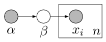
(a) (b)

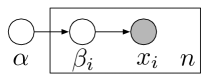
Figure 1: (a) A graphical model for a standard Bayesian model (b) A graphical model for a localized model. By drawing a new parameter $\beta_{i}$ for each data point, the localized model allows individual data points to vary more than the standard Bayesian model as in (a). Note the robust model requires that we fit the hyperparameter $\alpha$. Otherwise the data are rendered completely independent.

We first describe standard Bayesian modeling, and the key ingredients that we will build on. We then develop robust Bayesian modeling.

2.1 Bayesian models

Bayesian modeling uses probability to capture uncertainty around unknown parameters in a statistical model (Gelman et al., 2003). A Bayesian model is a joint distribution of parameters $\beta$ and a data set $\mathbf{x}$. In an exchangeable model, this joint factorizes into a product of likelihood terms for each data point $p(x_{i}\,|\,\beta)$ and a prior of the parameters $p(\beta\,|\,\alpha)$ (Equation 1.1). The prior is governed by the hyperparameter $\alpha$.

Figure 1 (a) shows the graphical model. This model easily generalizes to include conditional models, such as in Bayesian linear regression and logistic regression (Bishop, 2006), local latent variables, such as in Bayesian mixtures (Corduneanu and Bishop, 2001) and topic models (Blei et al., 2003; Blei, 2012), and non-exchangeable data, such as in a hidden Markov model (Rabiner, 1989) or Kalman filter (Kalman, 1960). For now we focus on the simplest setting in Equation 1.1.

When we use a model we condition on data and compute the corresponding posterior, the conditional distribution of the parameter given the data. We then employ the posterior in an application, such as to form predictions or to investigate properties of the data.

The posterior is proportional to the product of the prior and the data likelihood,

$$p(\beta\,|\,\mathbf{x},\alpha)\propto p(\beta\,|\,\alpha)\prod_{i=1}^{n}p(x_{i}\,|\,\beta).$$ (2.1)

We can use the posterior to form the posterior predictive distribution, the distribution of a new data point conditional on the observed data. The posterior predictive distribution is

$$p(x_{\mathrm{new}}\,|\,\mathbf{x},\alpha)=\int p(x_{\mathrm{new}}\,|\,\beta)p(\beta\,|\,\mathbf{x},\alpha)\mathrm{d}\beta.$$ (2.2)

It integrates the data likelihood $p(x_{\mathrm{new}}\,|\,\beta)$ under the posterior distribution $p(\beta\,|\,\mathbf{x},\alpha)$. The posterior predictive distribution is an important idea in Bayesian modeling. It is used both to form predictions about the future and to check, diagnose, and select models (Geisser and Eddy, 1979; Rubin, 1984; Gelman et al., 1996).

2.2 Robust Bayesian models

One of the virtues of Bayesian modeling is that the model’s prediction about the future does not rely on a single point estimate of the parameter, and averaging over the posterior can mitigate overfitting. However, the Bayesian pipeline does not explicitly aim for a good predictive distribution on future data—the posterior predictive of Equation 2.2 is the true distribution of unseen data only when the chosen model represents the true distribution of the data (Bernardo and Smith, 1994).

In practice, we use models to simplify a complex data generating process (Box, 1980). Thus there is always a mismatch between the posterior predictive distribution and the true distribution of future data. This motivates the philosophy behind robust statistics (Huber and Ronchetti, 2009), which aims to develop methods that are not sensitive to small changes in the modeling assumptions.

We develop robust Bayesian models, models that can usefully accommodate deviation from the underlying assumptions. We will use two ideas: localization and empirical Bayes.

The localized model.  The first idea is localization. As we discussed above, a traditional Bayesian model independently draws the data $\mathbf{x}$ conditional on the parameter $\beta$, which is drawn from the prior. The localized model relaxes this to a hierarchical model, which governs each data point with an individual parameter $\beta_{i}$ that is drawn from the prior. In Equation 1.2, the joint distribution of the individualized parameters $\bm{\beta}=\beta_{1:n}$. The localized model captures heterogeneity in the data; it explains atypical data that deviates from the norm (i.e., outliers) by deviations in their parameters.

One way to view the localized model is as one where each data point is drawn independently and identically distributed (IID) from an integrated likelihood,

$$p(x_{i}\,|\,\alpha)=\int p(x_{i}\,|\,\beta_{i})p(\beta_{i}\,|\,\alpha)\mathrm{d}\beta_{i}.$$ (2.3)

When the parameter $\beta_{i}$ controls the dispersion of the data, this results in a heavier-tailed distribution than the original (unintegrated) observation model in Equation 1.1.

For example, suppose the original model assumes data are from a Gaussian distribution. Localizing the variance under an inverse gamma prior reveals the student’s t-distribution, a commonly-used distribution for adding robustness to models of continuous data (Gelman et al., 2003). In Section 3 we show that many methods in robust statistics can be interpreted in this way.

Empirical Bayes estimation.  Crucially, localization requires that we infer the hyperparameter—it is now $\alpha$ that carries common information about the data. We can see this graphically. Localization takes us from the traditional Bayesian model in Figure 1 (a) to the model in Figure 1 (b). In Figure 1 (b), fixing $\alpha$ renders the data completely independent.

We fit the hyperparameter with maximum likelihood. This amounts to finding a prior on $\beta_{i}$ that maximizes the integrated likelihood of the data in in the robust model,

$$\hat{\alpha}=\arg\max_{\alpha}\sum_{i=1}^{n}\log\int p(x_{i}\,|\,\beta_{i})p(\beta_{i}\,|\,\alpha)\mathrm{d}\beta_{i}.$$ (2.4)

Here we marginalize out the individualized parameters $\beta_{i}$ from Equation 1.2. Thus fitting a robust model implicitly optimizes the predictive distribution.

Directly optimizing the likelihood can be difficult because of the integral inside the log function. We defer this issue to Section 4, where we show how to optimize with a combination of variational inference (Jordan et al., 1999) and the expectation maximization algorithm (Dempster et al., 1977). Our approach—localizing a global variable and then fitting its prior—allows us to develop robust variants of many Bayesian models. As we mentioned in the introduction, this perspective has close connections to empirical Bayes (Efron and Morris, 1973, 1975; Efron, 2010) and the empirical Bayes approach laid out in Carlin and Louis (2000a).

The predictive distribution.  With a localized model and estimated hyperparameter, we form predictions about future data with the corresponding predictive distribution

$$p(x^{*}\,|\,\hat{\alpha})=\int p(x^{*}\,|\,\beta^{*})p(\beta^{*}\,|\,\hat{\alpha}){\rm d}\beta^{*}.$$

Notice this has the same form as the likelihood term in the objective of Equation 2.4.

This predictive procedure motivates our approach to localize parameters and then fit hyperparameters with empirical Bayes. One goal of Bayesian modeling is to make better predictions about unseen data by using the integrated likelihood, and the traditional Bayesian approach of Equation 2.2 is to integrate relative to the posterior distribution. For making predictions, however, the traditional Bayesian approach is mismatched because the posterior is not formally optimized to give good predictive distributions of each data point. As we mentioned, it is only the right procedure when the data comes from the model (Bernardo and Smith, 1994).

In contrast, the robust modeling objective of Equation 2.4—the objective that arises from localization and empirical Bayes—explicitly values a distribution of $\beta$ that gives good predictive distributions for each data point, even in the face of model mismatch.

3 Practicing Robust Bayesian Modeling

Machine learning and Bayesian statistics have produced a rich constellation of Bayesian models and general algorithms for computing about them (Gelman et al., 2003; Bishop, 2006; Murphy, 2013). We have described an approach to robustifying Bayesian models in general, without specifying a model in particular. The recipe is to form a model, localize its parameters, and then fit the hyperparameters with empirical Bayes. In Section 4, we will develop general algorithms for implementing this procedure. First we describe some of the types of models that an investigator may want to make robust, and give some concrete examples.

First, many models contain hidden variables within $p(x_{i}\,|\,\beta)$, termed local variables in Hoffman et al. (2013). Examples of local variables include document-level variables in topic models (Blei et al., 2003), component assignments in mixture models (McLachlan and Peel, 2000), and per-data point component weights in latent feature models (Salakhutdinov and Mnih, 2008). We will show how to derive and compute with robust versions of Bayesian models with local hidden variables. For example, the bursty topic models of Doyle and Elkan (2009) and the robust mixture models of Peel and McLachlan (2000) can be seen as variants of robust Bayesian models.

Second, some models contain two kinds of parameters, and the investigator may only want to localize one of them. For example the Gaussian is parameterized by a mean and variance. Robust Gaussian model need only localize the variance; this results in the student’s t-distribution. In general, these settings are straightforward. Divide the parameter into two parts $\beta=[\beta_{1},\beta_{2}]$ and form a prior that divides similarly $\alpha=[\alpha_{1},\alpha_{2}]$. Localize one of the parameters and estimate its corresponding hyperparameter.

Last, many models are not fully generative, but draw each data point conditional on covariates. Examples include linear regression, logistic regression, and all other generalized linear models (McCullagh and Nelder, 1989). This setting is also straightforward in our framework. We will show how to build robust generalized linear models, such as Poisson regression and logistic regression, and how to fit them with our algorithm.

We now show how to build robust versions of several types of Bayesian models. These models connect to existing robust methods in the research literature, each one originally developed on a case-by-case basis.

3.1 Conjugate exponential families

The simplest Bayesian model draws data from an exponential family and draws its parameter from the corresponding conjugate prior. The density of the exponential family is

$$p(x\,|\,\eta)=h(x)\exp\left\{\eta^{\top}t(x)-a_{x}(\eta)\right\},$$

where $t(x)$ is the vector of sufficient statistics, $\eta$ is the natural parameter, and $h(x)$ is the base measure. The log normalizer $a_{x}(\eta)$ ensures that the density integrates to one,

$$a_{x}(\eta)=\int\exp\left\{\eta^{\top}t(x)\right\}\mathrm{d}x.$$ (3.1)

The density is defined by the sufficient statistics and natural parameter. When $x_{i}$ comes from an exponential family we use the notation $x_{i}\sim\textsc{ExpFam}(\eta,t(x))$.

Every exponential family has a conjugate prior (Diaconis and Ylvisaker, 1979). Suppose the data come from $x_{i}\sim\textsc{ExpFam}(\eta,x)$, i.e., the exponential family where $x$ is its own sufficient statistic. The conjugate prior on $\eta$ is

$$p(\eta\,|\,\alpha)=h(\eta)\exp\left\{\alpha^{\top}[\eta,-a_{x}(\eta)]-a_{\eta}(\alpha)\right\}.$$

This is an exponential family whose sufficient statistics concatenate the parameter $\eta$ and the negative log normalizer $-a_{x}(\eta)$ in the likelihood of the data. The parameter divides into two components $\alpha=[\alpha_{1},\alpha_{2}]$ where $\alpha_{1}$ has the same dimension as $\eta$ and $\alpha_{2}$ is a scalar. Note the difference between the two log normalizers: $a_{x}(\eta)$ normalizes the data likelihood; $a_{\eta}(\alpha)$ normalizes the prior. In our notation, $\eta\sim\textsc{ExpFam}([\alpha_{1},\alpha_{2}],[\eta,-a_{x}(\eta)])$.

Given data $\mathbf{x}$, the posterior distribution of $\eta$ is in the same exponential family as the prior,

$$\eta\,|\,\mathbf{x},\alpha\sim\textsc{ExpFam}\left([\alpha_{1}+\textstyle\sum_{i}x_{i},\alpha_{2}+n],[\eta,-a_{x}(\eta)]\right).$$ (3.2)

This describes the general set-up behind all commonly used conjugate prior-likelihood pairs, such as the Beta-Bernoulli, Dirichlet-Multinomial, Gamma-Poisson, and others. Each of these models first draws a parameter $\eta$ from a conjugate prior, and then draws $n$ data points $x_{i}$ from the corresponding exponential family.

Following Section 2.2, we define a generic localized conjugate exponential family,

$$\eta_{i} \sim\textsc{ExpFam}\left([\alpha_{1},\alpha_{2}],[\eta,-a_{x}(\eta)]\right)$$

$$x_{i} \sim\textsc{ExpFam}\left(\eta_{i},x\right).$$

We fit the hyperparameters $\alpha$ to maximize the likelihood of the data in Equation 2.4. In a conjugate exponential-family pair, the integrated likelihood has a closed form expression. It is a ratio of normalizers,

$$p(x_{i}\,|\,\alpha) =\int p(x_{i}\,|\,\eta)p(\eta\,|\,\alpha)\mathrm{d}\eta$$

$$=\exp\left\{a_{\eta}([\alpha_{1}+x_{i},\alpha_{2}+1])-a_{\eta}([\alpha_{1},\alpha_{2}])\right\}.$$ (3.3)

In this setting the log likelihood of Equation 2.4 is

$$\mathcal{L}(\alpha_{1},\alpha_{2};\mathbf{x})=\left(\textstyle\sum_{i=1}^{n}a_{\eta}(\alpha_{1}+x_{i},\alpha_{2}+1)\right)-na_{\eta}(\alpha_{1},\alpha_{2}).$$

This general story connects to specific models in the research literature. As we described above, it leads to the student’s t-distribution when the data come from a Gaussian with a fixed mean and localized variance $x_{i}\sim\mathcal{N}(\mu,\sigma_{i}^{2})$, and when the variance $\sigma^{2}_{i}$ has an inverse Gamma prior. It is “robust” when the dispersion parameter is individualized; the model can explain outlier data by a large dispersion. Fitting the hyperparameters amounts to maximum likelihood estimation of the student’s t-distribution.

This simple exchangeable model also connects to James-Stein estimation, a powerful method from frequentist statistics that can be understood as an empirical Bayes procedure (Efron and Morris, 1973; Efron, 2010). Here the data are from a Gaussian with fixed variance and localized mean $x_{i}\sim\mathcal{N}(\mu_{i},\sigma^{2})$, and the mean $\mu_{i}$ has a Gaussian prior $\mu_{i}\sim\mathcal{N}(0,\lambda^{2})$. (This is the conjugate prior.) We recover a shrinkage estimate similar to James-Stein estimation by fitting the prior variance with maximum likelihood.

3.2 Generalized linear models

Generalized linear models (GLM) are conditional models of a response variable $y$ given a set of covariates $x$ (McCullagh and Nelder, 1989). Specifically, canonical GLMs assume the response is drawn from an exponential family with natural parameters equal to a linear combination of coefficients $w$ and covariates.

$$\eta_{i} =w^{\top}x_{i}$$

$$y_{i} \sim\textsc{ExpFam}(\eta_{i},y).$$

Many conditional models are generalized linear models; some of the more common examples are linear regression, logistic regression, and Poisson regression. For example, Poisson regression sets $\eta_{i}=w^{\top}x_{i}$ to be the log of the rate of the Poisson distribution of the response. (This fits our notation—the log of the rate is the natural parameter of the Poisson.)

We use the method from Section 2.2 to construct a robust GLM. We replace the deterministic natural parameter with a Gaussian random variable,

$$\eta_{i} \sim\mathcal{N}(w^{\top}x_{i},\lambda^{2}).$$

Its mean is the linear combination of coefficients and covariates, and we fit the coefficients $w$ and variance $\lambda^{2}$ with maximum likelihood. This model captures heterogeneity among the response variables. It accommodates outliers and enables more robust estimation of the coefficients.

Unlike Section 3.1, however, this likelihood-prior pair is typically not conjugate—the conditional distribution of $\eta_{i}$ will not be a Gaussian and the integrated likelihood is not available in closed form. We will handle this nonconjugacy with the algorithms in Section 4.

In our examples we will always use Gaussian priors. However, we can replace them with other distributions of the reals. We can interpret the choice of prior as a regularizer on a per-data point “shift parameter.” This is the idea behind She and Owen (2011) (for linear regression) and Tibshirani and Manning (2013) (for logistic regression). These papers set up a shift parameter with $L_{1}$ regularization, which corresponds to a Laplace prior in the models described here.

We give two examples of robust generalized linear models: robust logistic regression and robust Poisson regression. (We discuss robust linear regression below, when we develop robust overdispersed GLMs.)

Example: Robust logistic regression.  In logistic regression $y_{i}$ is a binary response,

$$y_{i}\sim\mathrm{Bernoulli}(\sigma(w^{\top}x_{i}))$$

where $\sigma(t)=(1+\exp(-t))^{-1}$ is the logistic function; it maps the reals to the unit interval.

We apply localization to form robust logistic regression. The model is

$$\eta_{i} \sim\mathcal{N}(w^{\top}x_{i},\lambda^{2})$$

$$y_{i} \sim\mathrm{Bernoulli}(\sigma(\eta_{i})),$$

where we estimate $w$ and $\lambda^{2}$ by maximum likelihood. This model is robust to outliers in the sense that the per-data distribution on $\eta_{i}$ allows individual data to be “misclassified” by the model. As we mentioned for the general case, the Gaussian prior is not conjugate to the logistic likelihood; we can use the approximation algorithm in Section 4 to compute with this model.

We note that there are several existing variants of robust logistic regression. Pregibon (1982) and Stefanski et al. (1986) use M-estimators (Huber, 1964) to form more robust loss functions, which are designed to reduce the contribution from possible outliers. Our approach can be viewed as a likelihood-based robust loss function, where we integrate the likelihood over the individual parameter $\beta_{i}$. This induces uncertainty around individual observations, but without explicitly defining the form of a robust loss.

Closer to our method is the shift model of Tibshirani and Manning (2013), who use $L_{1}$ regularization, as well as the more recent theoretical work of Feng et al. (2014). However, none of this work estimates hyperparameters $\lambda$. Using empirical Bayes to estimating such hyperparameters is at the core of our procedure, and we found in practice that it is an important component.

Example: Robust Poisson regression.  The Poisson distribution is an exponential family on positive integers. Its parameter is a single a positive value, the rate. Poisson regression is a conditional model of a count-valued response,

$$y_{i}\sim\mathrm{Poisson}\left(\exp\left\{w^{\top}x_{i}\right\}\right).$$

Using localization, a robust Poisson regression model is

$$\eta_{i} \sim\mathcal{N}(w^{\top}x_{i},\lambda^{2})$$ (3.4)

$$y_{i} \sim\mathrm{Poisson}\left(\exp\left\{\eta_{i}\right\}\right).$$ (3.5)

As for all the models above, this allows individual data points to deviate from their expected value. Notice this is particularly important when the data are Poisson, where the variance equals the mean. In classical Poisson regression, the mean is $\mathbb{E}[Y_{i}\,|\,x_{i}]=w^{\top}x_{i}$ and the variance is $\mathrm{Var}[Y_{i}\,|\,x_{i}]=w^{\top}x_{i}$. Here we can marginalize out the per-data point parameter in the robust model to reveal a larger variance,

$$\mathbb{E}[Y_{i}\,|\,x_{i}] =\exp\left\{w^{\top}x_{i}+\lambda^{2}/2\right\}$$

$$\mathrm{Var}[Y_{i}\,|\,x_{i}] =\exp\left\{w^{\top}x_{i}+\lambda^{2}/2\right\}+\left(\exp\left\{\lambda^{2}\right\}-1\right)\exp\left\{2w^{\top}x_{i}+\lambda^{2}\right\}.$$

These marginal moments comes from the fact that $\exp\left\{w^{\top}x_{i}\right\}$ follows a log normal. Intuitively, as the prior variance $\lambda^{2}$ goes to zero they approach the moments for classical Poisson regression.

Robust Poisson regression relates to negative binomial regression (Cameron and Trivedi, 2013), which also introduces per-data flexibility. Negative binomial regression is

$$\epsilon_{i} \sim\mathrm{Gamma}(a,b)$$

$$\eta_{i} =w^{\top}x_{i}+\log\epsilon_{i}$$

$$y_{i} \sim\textrm{Poisson}(\exp\left\{\eta_{i}\right\}).$$

In this notation, this model assumes that $\epsilon_{i}$ drawn from a Gamma distribution and further estimates its parameters with empirical Bayes. In our study, we found that the robust Poisson model defined in Equations 3.4 and 3.5 outperformed negative binomial regression; we suspect this is because of the empirical Bayes step. (See Section 5.)

3.3 Overdispersed generalized linear models

An overdispersed exponential family extends the exponential family with a dispersion parameter, a positive scalar that controls the variance. An overdispersed exponential family is

$$p(y\,|\,\eta,\tau)=h(y,\tau)\exp\left\{\frac{\eta^{\top}t(y)-a_{y}(\eta)}{\tau}\right\},$$ (3.6)

where $\tau$ is the dispersion. We denote this $y\sim\textsc{OvExpFam}(\eta,t(y),\tau)$. One example of an overdispersed exponential family is the Gaussian—the parameter $\eta$ is the mean and $\tau$ is the variance. (We can also form a Gaussian in a standard exponential family form, where the natural parameter combines the mean and the variance.)

An overdispersed GLM draws the response from an overdispersed exponential family (Jorgensen, 1987). Following Section 3.1, we localize the dispersion parameter $\tau$ to create a robust overdispersed GLM. In this case we draw $\tau$ from a Gamma,

$$\tau_{i} \sim\textrm{Gamma}(a,b)$$

$$y_{i} \sim\textsc{OvExpFam}(w^{\top}x_{i},y_{i},\tau_{i})$$

Localizing the dispersion connects closely with our intuitions around robustness. An outlier is one that is overdispersed relative to what the model expects; thus a per-data point dispersion parameter can easily accommodate outliers.

For example consider the GLM that uses a unit-variance Gaussian with unknown mean (an exponential family). This is classical linear regression. Now form the overdispersed GLM—this is linear regression with unknown variance—and localize the dispersion parameter under the Gamma prior. Marginalizing out the per-data dispersion, this model draws the response from a student’s t,

$$y_{i}\sim t_{2a}(\cdot\,|\,w^{\top}x_{i},1/(ab))$$

where the student’s t notation ${\rm t}_{\nu}(y\,|\,\mu,\phi)$ is

$$t_{\nu}(y|\mu,\phi)=\frac{\Gamma(\frac{\nu+1}{2})}{\Gamma(\frac{\nu}{2})\sqrt{\pi\nu\phi}}\left(1+\frac{1}{\nu}\frac{(y-\mu)^{2}}{\phi}\right)^{-\frac{\nu+1}{2}}.$$

This is a robust linear model, an alternative parameterization of the model of Lange et al. (1989) and Fernández and Steel (1999).

Intuitively, localized overdispersed models lead to heavy-tailed distributions because it is the dispersion that varies from data point to data point. When working with the usual exponential family (as in Section 3.1 and Section 3.2), the heavy-tailed distribution arises only when the dispersion is contained in the natural parameter; note this is the case for our previous examples, logistic regression and Poisson regression. Here, the dispersion is localized by design.

3.4 Generative models with local and global variables

We have described how to build robust versions of simple models—conjugate prior-exponential families, generalized linear models, and overdispersed generalized linear models. Modern machine learning and Bayesian statistics, however, has developed much more complex models, using exponential families and GLMs as components in structured joint distributions (Bishop, 2006; Murphy, 2013). Examples include models of time series, hierarchies, and mixed-membership. We now describe how to use the method of Section 3.1 build robust versions of such models.

Each complex Bayesian model is a joint distribution of hidden and observed variables. Hoffman et al. (2013) divide the variables into two types: local variables $\mathbf{z}$ and global variables $\beta$. Each local variable $z_{i}$ helps govern of its associated data point $x_{i}$ and is conditionally independent of the other local variables. In contrast, the global variables $\beta$ help govern the distribution of all the data. This is expressed in the following joint,

$$p(\beta,\mathbf{z},\mathbf{x})=p(\beta)\prod_{i=1}^{n}p(z_{i},x_{i}\,|\,\beta).$$

This joint describes a wide class of models, including Bayesian mixture models (Ghahramani and Beal, 2000; Attias, 2000), hierarchical mixed membership models (Blei et al., 2003; Erosheva et al., 2007; Airoldi et al., 2007), and Bayesian nonparametric models (Antoniak, 1974; Teh et al., 2006).

To make a robust Bayesian model, we localize some of its global variables—we bring them inside the likelihood of each data point, endowing each with a prior, and then fit that prior with empirical Bayes. Localizing global variables accommodates outliers by allowing how each data point expresses the global patterns to deviate from the norm. Figure 2 shows the graphical model where $\beta_{i}$ is the localized global variable and $z_{i}$ is the original local variable.

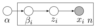
Figure 2: Robust modeling with with local latent variable $\beta_{i}$, $z_{i}$ and observation $x_{i}$, $i=1,\dots,n$.

As an example, consider latent Dirichlet allocation (LDA) (Blei et al., 2003). LDA is a mixed-membership model of a collection of documents; each document is a collection of words. LDA draws each document from a mixture model, where the mixture proportions are document-specific and the mixture components (or “topics”) are shared across the collection.

Formally, define each topic $\beta_{k}$ to be a distribution over a fixed vocabulary and fix the number of topics $K$. LDA assumes that a collection of documents comes from the following process:

1. Draw topic $\beta_{k}\sim\mathrm{Dir}(\eta)$ for $k=1,2,\cdots,K$.

2. For each document $d$,

   1. Draw topic proportions $\theta_{d}\sim\mathrm{Dir}(\alpha)$.

   2. For each word $n$,

      1. Draw topic assignment $z_{dn}\sim\mathrm{Mult}(\theta_{d})$.

      2. Draw word $w_{dn}\sim\mathrm{Mult}(\beta_{z_{dn}})$.

The local variables are the topic assignments and topic proportions; they are local to each document. The global variables are the topics; they are involved in the distribution of every document.

For simplicity, denote steps (a) and (b) above as $\mathbf{w}_{d}\sim\mathrm{LDA}(\bm{\beta},\alpha)$, where $\bm{\beta}=\{\beta_{1},\ldots,\beta_{K}\}$. To make LDA robust, we localize the topics. Robust LDA still draws each document from a mixture of $K$ topics, but the topics are themselves drawn anew for each document.

Each per-document topic $\beta_{dk}$ is drawn from its own distribution with a “master” topic parameter $\eta_{k}$, which parameterizes the Dirichlet of the $k$-th topic. Localized LDA draws each document from the following process:

1. Draw per-document topic $\beta_{dk}\sim\mathrm{Dir}(\eta_{k})$, for $k=1,2,\cdots,K$.

2. Draw $\mathbf{w}_{d}\sim\mathrm{LDA}(\bm{\beta}_{d},\alpha)$.

We fit the hyperparameters $\eta_{k}$, the corpus-wide topics. In the generative process they are perturbed to form the per-document topics.

This robust LDA model is equivalent to the topic model proposed in Doyle and Elkan (2009), which accounts for “burstiness” in the distribution of words of each documents. Burstiness, also called contagion, is the idea that when we see one word in a document we are more likely to see that word again. It is a property of the marginal distribution of words when integrating out a Dirichlet distributed multinomial parameter. This is called a Dirichlet-multinomial compound distribution (Madsen et al., 2005).

Burstiness is a good property in topic models. In a traditional topic model, repeated terms provide increased evidence for the importance of that term in its topic. In contrast, the bursty topic model can partly explain repeated terms by burstiness. Consequently, the model does not overestimate that term’s importance in its topic.

LDA is just one example. With this method we can build robust versions for mixtures, time-series models, Bayesian nonparametric models, and many others. As for GLMs, we have a choice of what to localize. In topic models we localized the topics, resulting in a bursty topic model. In other cases we localize dispersion parameters, such as in robust Gaussian mixtures (Svensén and Bishop, 2005).

4 Fitting robust Bayesian models

We have shown how to robustify a wide class of Bayesian models. The remaining question is how to analyze data with them. We now show how to adapt existing approximate inference algorithms to compute with robust Bayesian models. We provide a general strategy that can be used with simple models (e.g., conjugate exponential families), nonconjugate models (e.g., generalized linear models), and complex models with local and global variables (e.g., LDA).

The key algorithmic problem is to fit the hyperparameter in Equation 2.4. We use an expectation-maximization (EM) algorithm to fit the model (Dempster et al., 1977). In many cases, some of the necessary quantities are intractable to compute. We approximate them with variational methods (Jordan et al., 1999; Wainwright and Jordan, 2008).

Consider a generic robust Bayesian model. The data come from an exponential family and the parameter from a general prior,

$$\beta_{i} \sim p(\cdot\,|\,\alpha)$$

$$x_{i} \sim\textsc{ExpFam}(x_{i},\beta_{i}).$$

Note this is not necessarily the conjugate prior. Following Section 2.2, we fit the hyperparameters $\alpha$ according to Equation 2.4 to maximize the marginal likelihood of the data.

We use a generalization of the EM algorithm, derived via variational methods. Consider an arbitrary distribution of the localized variables $q(\beta_{1:n})$. With Jensen’s inequality, we use this distribution to bound the marginal likelihood. Accounting for the generic exponential family, the bound is

$$\mathcal{L}(\alpha) \geq\sum_{i=1}^{n}\mathbb{E}_{q}\left[\log p(x_{i}\,|\,\beta_{i})p(\beta_{i}\,|\,\alpha)\right]-\mathbb{E}_{q}\left[\log q(\beta_{i})\right]$$

$$=\sum_{i=1}^{n}\mathbb{E}_{q}\left[\beta_{i}\right]^{\top}x_{i}-\mathbb{E}_{q}\left[a(\beta_{i})\right]+\mathbb{E}_{q}\left[\log p(\beta_{i}\,|\,\alpha)\right]-\mathbb{E}_{q}\left[\log q(\beta_{i})\right].$$ (4.1)

This is a variational bound on the marginal likelihood (Jordan et al., 1999), also called the ELBO (“the Evidence Lower BOund”). Variational EM optimizes the ELBO by coordinate ascent—it iterates between optimizing with respect to $q(\beta_{1:n})$ and with respect to the hyperparameters $\alpha$.

Optimizing Equation 4.1 with respect to $q(\beta_{1:n})$ minimizes the Kullback-Leibler divergence between $q(\beta_{1:n})$ and the exact posterior $p(\beta_{1:n}\,|\,\mathbf{x})$.

In a localized model, the posterior factorizes,

$$p(\beta_{1:n}\,|\,\mathbf{x},\alpha)=\prod_{i=1}^{n}p(\beta_{i}\,|\,x_{i},\alpha).$$

Each factor is a posterior distribution of the per-data point parameter, conditional on the data point and the hyperparameters. If each posterior factor is computable then we can perform an exact E-step, where we set $q(\beta_{i})$ equal to the exact posterior. In the context of empirical Bayes models, this is the algorithm suggested by Carlin and Louis (2000a).

In many cases the exact posterior will not be available. In these cases we use variational inference (Jordan et al., 1999). We set $q(\beta_{i})$ to be a parameterized family of distributions over the $i$th variable $\beta_{i}$ and then optimize Equation 4.1 with respect to $q(\cdot)$. This is equivalent to finding the distributions $q(\beta_{i})$ that are closest in KL divergence to the exact posteriors $p(\beta_{i}\,|\,x_{i},\alpha)$. It is called a variational E-step.

The M-step maximizes Equation 4.1 with respect to the hyperparameter $\alpha$. It solves the following optimization problem,

$$\hat{\alpha}=\arg\max_{\alpha}\sum_{i=1}^{n}\mathbb{E}_{q}\left[\log p(\beta_{i}\,|\,\alpha)\right].$$ (4.2)

At first this objective might look strange—the data do not appear. But the expectation is taken with respect to the (approximate) posterior $p(\beta_{i}\,|\,x_{i},\alpha)$ for each localized parameter $\beta_{i}$; this posterior summarizes the $i$th data point. We solve this optimization with gradient methods.

Nonconjugate models.  As we described, the E-step amounts to computing $p(\beta_{i}\,|\,x_{i},\alpha)$ for each data point. When the prior and likelihood form a conjugate-pair (Section 3.1) then we can compute an exact E-step. For many models, however, the E-step is not computable and we need to approximate $p(\beta_{i}\,|\,x_{i},\alpha)$.

One type of complexity comes from nonconjugacy, where the prior is not conjugate to the likelihood. As a running example, robust GLM models (Section 3.2) are generally nonconjugate. (Robust linear regression is an exception.) In a robust GLM, the goal is to find optimal coefficients $w$ and variance $\lambda^{2}$ that maximizes the robust GLM ELBO,

$$\mathcal{L}(w,\alpha)=\sum_{i=1}^{n}\mathbb{E}_{q}\left[\eta_{i}\right]^{\top}y_{i}-\mathbb{E}_{q}\left[a(\eta_{i})\right]+\mathbb{E}_{q}\left[\log p(\eta_{i}\,|\,w^{\top}x_{i},\lambda^{2})\right]-\mathbb{E}_{q}\left[\log q(\eta_{i})\right].$$ (4.3)

The latent variables are $\eta_{i}$, the per-data point natural parameters. Their priors are Gaussians, each with mean $w^{\top}x_{i}$ and variance $\lambda^{2}$.

In an approximate E-step, we hold the parameters $w$ and $\lambda^{2}$ fixed and approximate the per-data point posterior $p(\eta_{i}\,|\,y_{i},x_{i},w,\lambda^{2})$. In theory, the optimal variational distribution (Bishop, 2006) is

$$q(\eta_{i})\propto\exp\left(\eta_{i}y_{i}-a(\eta_{i})+\log p(\eta_{i}\,|\,w^{\top}x_{i},\alpha)\right).$$

But this does not easily normalize.

We address the problem with Laplace variational inference (Wang and Blei, 2013). Laplace variational inference approximates the optimal variational distribution with

$$q(\eta_{i})\approx\mathcal{N}(\hat{\eta}_{i},-h^{-1}(\hat{\eta}_{i})).$$ (4.4)

The value $\hat{\eta}_{i}$ maximizes the following function,

$$f(\eta_{i})=\eta_{i}y_{i}-a(\eta_{i})+\log p(\eta_{i}\,|\,w^{\top}x_{i},\lambda^{2}),$$ (4.5)

where $h(\cdot)$ is the Hessian of that function. Finding the $\hat{\eta}_{i}$ can be done using many off-the-shelf optimization routines, such as conjugate gradient.

Given these approximations to the variational distribution, the M-step estimates $w$ and $\alpha$,

$$[\hat{w},\hat{\alpha}]=\arg\max_{w,\alpha}\sum_{i=1}^{n}\mathbb{E}_{q(\eta_{i})}\left[\log p(\eta_{i}\,|\,w^{\top}x_{i},\alpha)\right].$$ (4.6)

In robust GLMs, the prior is Gaussian and we can compute the expectation in closed form. In general nonconjugate models, however, we may need to approximate the expectation. Here we use the multivariate delta method to approximate the objective (Bickel and Doksum, 2007; Wang and Blei, 2013). Algorithm 1 shows the algorithm.

Initialize $w$ and $\alpha$.

repeat

       for $i\in\{1,2,\dots,n\}$ do

             Update variational distribution $q(\eta_{i})$ (Equation 4.4).

       end for

      Update $w$ and $\alpha$ using gradient ascent (Equation 4.6).

until the ELBO converges.

Algorithm 1 Variational EM for a robust GLM.

Complex models with local and global variables.  We can also use variational inference when we localize more complex models, such as mixture models or topic models. Here we outline a strategy that roughly follows Hoffman et al. (2013).

We discussed complex Bayesian models in Section 3.4; see Figure 2. Observations are $x_{1:n}$ and local latent variables are $z_{1:n}$ and $\beta_{1:n}$. (We have localized the global variable $\beta$.) The joint distribution is

$$p(\beta_{1:n},x_{1:n},z_{1:n},\,|\,\alpha)=\textstyle\prod_{i=1}^{n}p(\beta_{i}\,|\,\alpha)p(z_{i},x_{i}\,|\,\beta_{i}).$$ (4.7)

Assume these distributions are in the exponential family,

$$p(z_{i},x_{i}\,|\,\beta_{i}) \textstyle=h_{\ell}(z_{i},x_{i})\exp\left\{\beta_{i}^{\top}t_{\ell}(z_{i},x_{i})-a_{\ell}(\beta_{i})\right\}$$ (4.8)

$$p(\beta_{i}\,|\,\alpha) \textstyle=h(\beta_{i})\exp\left\{\alpha^{\top}t(\beta_{i})-a(\alpha)\right\},$$ (4.9)

The term $t(\beta_{i})$ has the form $t(\beta_{i})=[\beta_{i},-a_{\ell}(\beta_{i})]$. It is conjugate to $p(z_{i},x_{i}\,|\,\beta_{i})$.

This model satisfies conditional conjugacy. The conditional posterior $p(\beta_{i}\,|\,z_{i},x_{i})$ in the same family as the prior $p(\beta_{i}\,|\,\alpha)$. We emphasize that this differs from classical Bayesian conjugacy—when we marginalize out $z_{i}$ the posterior of $\beta_{i}$ is no longer in the same family.

The goal is to find the optimal $\alpha$ that maximizes the ELBO,

$$\mathcal{L}(\alpha) =\sum_{i=1}^{n}\mathbb{E}_{q}\left[\log p(x_{i},z_{i}\,|\,\beta_{i})\right]+\mathbb{E}_{q}\left[p(\beta_{i}\,|\,\alpha)\right]-\mathbb{E}_{q}\left[\log q(z_{1:n},\beta_{1:n})\right],$$ (4.10)

where the distribution $q(z_{1:n},\beta_{1:n})$ contains both types of latent variables.

We specify $q(\cdot)$ to be the mean-field family. It assumes a fully factorized distribution,

$$q(z_{1:n},\beta_{1:n}) =\textstyle\prod_{i=1}^{n}q(\beta_{i})q(z_{i}).$$ (4.11)

In the E-step we optimize the variational distribution. We iterate between optimizing $q(z_{i})$ and $q(\beta_{i})$ for each data point. Because of conditional conjugacy, these updates are in closed form,

$$q(\beta_{i}) \propto h(\beta_{i})\exp\left((\alpha+[\mathbb{E}_{q(z_{i})}\left[t(z_{i},x_{i})\right],1])^{\top}t(\beta_{i})\right),$$ (4.12)

$$q(z_{i}) \propto h(z_{i},x_{i})\exp\left(([t(z_{i},x_{i}),1])^{\top}\mathbb{E}_{q(\beta_{i})}\left[t(\beta_{i})\right]\right).$$ (4.13)

Each $q(\cdot)$ will be in the same exponential family as its complete conditional. For fixed $\alpha$, the variational distribution converges as we iterate between these updates.

In the M-step, we plug the fitted variational distributions into Equation 4.10 and optimize $\alpha$. Algorithm 2 shows the algorithm. This general method fits robust versions of complex models, such as bursty topic models or robust mixture models.

Initialize $\alpha$.

repeat

       for $i\in\{1,2,\dots,n\}$ do

             Update $q(\beta_{i})$ (Equation 4.12).

             Update $q(z_{i})$ (Equation 4.13).

            

       end for

      Plug $q(\beta_{i})$ and $q(z_{i})$ into Equation 4.10 and update parameter $\alpha$ with gradient ascent.

until the ELBO converges.

Algorithm 2 Variational EM for robust models with local and global variables.

5 Empirical Study

We study two types of robust Bayesian models—robust generalized linear models and robust topic models. We present results on both simulated and real-world data. We use the strategy of Section 4 for all models. We find robust models outperform their non-robust counterparts.

5.1 Robust generalized linear models

We first study the robust generalized linear models (GLMs) of Section 3.2 and Section 3.3—linear regression, logistic regression, and Poisson regression. Each involves modeling a response variable $y_{i}$ conditional on a set of covariates $x_{i}$. The response is governed (possibly through a localized variable) by a linear combination with coefficients $w^{\top}x_{i}$.

We study robust GLMs with simulated data. Our goal is to determine whether our method for robust modeling gives better models when the training data is corrupted by noise. The idea is to fit various models to corrupted training data and then evaluate those models on uncorrupted test data.

Each simulation involves a problem with five covariates. We first generated true coefficients $w$ (a vector with five components) from a standard normal; we then generated 500 test data points $(y_{i},x_{i})$ from the true model. For each data point, the five covariates are each drawn from $\mathrm{Unif}[-5,5]$ and the form of the response depends on which model we are studying. Next, we generate corrupted training sets, varying the amount of corruption. (How we corrupt the training set changes from problem to problem; see below.) Finally, we fit robust and non-robust models to each training set and evaluate their corresponding predictions on the test set. We repeat the simulation 50 times.

We found that robust GLMs form better predictions than traditional GLMs in the face of corrupted training data. Further, as expected, the performance gap increases as the training data is more corrupted.

Linear regression.  We first use simulated data to study linear regression. In the true model

$$y_{i}\,|\,x_{i}\sim\mathcal{N}(w^{\top}x_{i}+b,0.02).$$

In the corrupted training data, we set a noise level $k$ and generate data from

$$y_{i}\sim\mathcal{N}(w^{\top}x_{i}+b,\sigma_{i}+0.02),$$

where $\sigma_{i}\sim\mathrm{Gamma}(k,1)$. As $k$ gets larger, there are more outliers. We simulated training sets with different levels of outliers; we emphasize the test data does not include outliers.

We compare robust linear regression (with our general algorithm) to standard regression. After fitting coefficients $\hat{w}$ under the robust model, we form predictions on test data as for linear regression $\hat{y}_{\textrm{new}}=\hat{w}^{\top}x_{\mathrm{new}}$. We evaluate performance using three metrics: predictive L1,

$$\textstyle\mathrm{pL1}\triangleq 1-(\sum|y-\hat{y}|)/(\sum|y|),$$

predictive R2,

$$\textstyle\mathrm{pR2}\triangleq 1-(\sum(y-\hat{y})^{2})/(\sum y^{2}),$$

and the mean squared error to the true parameter (MSE)

$$\textstyle\mathrm{MSE}\triangleq(1/d)\sum_{i=1}^{d}(\hat{w}_{i}-w_{i})^{2},$$

where $d$ is the dimension of parameter $w$. Figure 3 shows the results. The robust model is better than standard linear regression when the training data is corrupted. This is consistent with the findings of Lange et al. (1989) and Gelman et al. (2003).

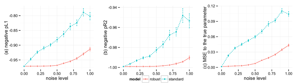
Figure 3: Robust linear regression compared to classical regression on simulated data. The x-axis is additional noise in the training data, not captured by the model or present in test data. Robust models perform better in the face of outliers. (a) Negative predictive L1; (b) Negative predictive R2. (c) MSE to the true parameter. For all metrics, lower is better.

Logistic regression.  We next study logistic regression. In the true model,

$$y_{i}\,|\,x_{i}\sim\mathrm{Bernoulli}(\sigma(w^{\top}x_{i})),$$

where $\sigma(\cdot)$ is the logistic function. To contaminate the training data, we randomly flip a percentage of the true labels, starting with those points close to the true decision boundary.

We compare robust logistic regression of Equations 3.4 and 3.5 to traditional logistic regression. Figure 4 shows the results. Robust models are better than standard models in terms of three metrics: classification error, negative predictive log likelihood, and mean square error (MSE) to the true data generating parameter $w$.

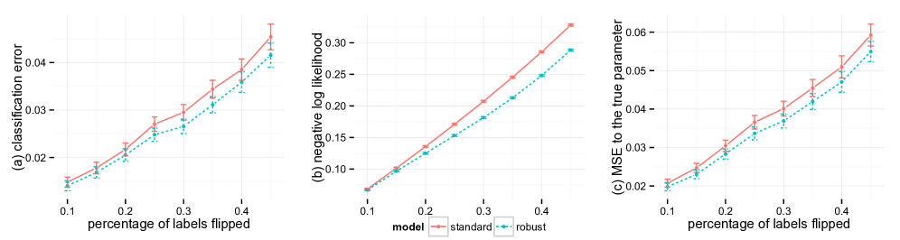
Figure 4: Experimental results for (robust) logistic regression on simulated data. Noise level (X-axis) indicates the proportion of the labels in the training data are flipped. (a) Classification error; (b) Negative predictive log likelihood. (c) MSE to the true parameter. All metrics: the lower the better. Robust model perform better when noise is presented.

Poisson regression.  Finally we study Poisson regression. In the true model

$$y_{i}\,|\,x_{i}\sim\mathrm{Poisson}\left(\exp\left\{w^{\top}x_{i}\right\}\right).$$

We corrupt the training data by sampling a per-data point noise component $\epsilon_{i}\sim\mathcal{N}(0,\sigma^{2})$ and then generating data from

$$y_{i}\,|\,x_{i}\sim\mathrm{Poisson}\left(\exp\left\{w^{\top}x_{i}+\epsilon_{i}\right\}\right).$$

The variance $\sigma^{2}$ controls the amount of noise in the training data.

We compare our robust Poisson regression to traditional Poisson regression and to negative binomial regression. Figure 5 shows the results. We used three metrics: predictive L1 (as for linear regression), negative predictive log likelihood, and MSE to the true coefficients. Robust models are better than both standard Poisson regression and the negative binomial regression, especially when there is large noise.

Note that negative binomial regression is also a robust model. In a separate study, we confirmed that it is the empirical Bayes step, where we fit the variance around the per-data point parameter, that explains our better performance. Using the robust Poisson model without fitting that variance (but still fitting the coefficients) gave similar performance to negative binomial regression.

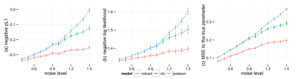
Figure 5: Experimental results for (robust) Poisson regression on simulated data. (a) Negative predictive L1; (b) Negative predictive log likelihood. (c) MSE to the true parameter. All metrics: the lower the better. Robust models tend to perform better than both Poisson regression and negative binomial regression (nb) when noise is presented.

Summary.  We summarize these experiments with Figure 6 showing the improvement of robust models over standard models in terms of log likelihood. (For linear regression, we use pR2.) Robust models give greater improvement when the data is noisier.

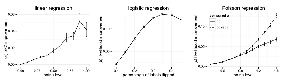
Figure 6: Improvement of robust models over standard models. (a) Predictive R2 improvement for linear regression; (b) log likelihood improvement for logistic regression (c) log likelihood improvement for Poisson regression.

5.2 Robust topic modeling

We also study robust LDA, an example of a complex Bayesian model (Section 3.4). We have discussed that robust LDA is a bursty topic model (Doyle and Elkan, 2009).

We analyze three document corpora: Proceedings of the National Academy of Sciences (PNAS), Science, and a subset of Wikipedia. The PNAS corpus contains 13,000 documents and has a vocabulary of 7,200 terms; the Science corpus contains 16,000 documents and has a vocabulary of 4,400 terms; the Wikipedia corpus contains about 10,000 documents and has a vocabulary of 15,300 terms. We run a similar study to the one in Doyle and Elkan (2009), comparing robust topic models to traditional topic models.

Evaluation metric.  To evaluate the methods, we hold out 20% documents from each corpus and calculate their predictive likelihood. We follow the metric used in recent topic modeling literature (Blei and Lafferty, 2007; Asuncion et al., 2009; Wang et al., 2011; Hoffman et al., 2013), where we hold out part of a document and predict its remainder.

Specifically, for each document in the test set $\mathbf{w}_{d}$, we split it in into two parts, $\mathbf{w}_{d}=[\mathbf{w}_{d1},\mathbf{w}_{d2}]$. We compute the predictive likelihood of $\mathbf{w}_{d2}$ given $\mathbf{w}_{d1}$ and $\mathcal{D}_{\rm train}$. The per-word predictive log likelihood is

$${{\rm likelihood}_{\rm pw}}\triangleq\frac{\sum_{d\in\mathcal{D}_{\rm test}}\log p(\mathbf{w}_{d2}|\mathbf{w}_{d1},\mathcal{D}_{\rm train})}{\sum_{d\in\mathcal{D}_{\rm test}}|\mathbf{w}_{d2}|},$$

where $|\mathbf{w}_{d2}|$ is the number of tokens in $\mathbf{w}_{d2}$. This evaluation measures the quality of the estimated predictive distribution. This is similar to the strategy used in Hoffman et al. (2013).

For standard LDA (Blei et al., 2003), conditioning on $\mathbf{w}_{d1}$ estimates the topic proportions $\theta_{d}$ from corpus-wide topics. These topic proportions are then used to compute the predictive likelihood of $\mathbf{w}_{d2}$. Robust LDA is different because conditioning on $\mathbf{w}_{d1}$ estimates both topic proportions and per-document topics; the predictive likelihood of $\mathbf{w}_{d2}$ uses both quantities.

Results.  Figure 7 shows the results. (Note, in the figure we use negative log likelihood so that it is consistent with other plots in this paper.) Robust topic models perform better than traditional topic models. This result is consistent with those reported in Doyle and Elkan (2009).

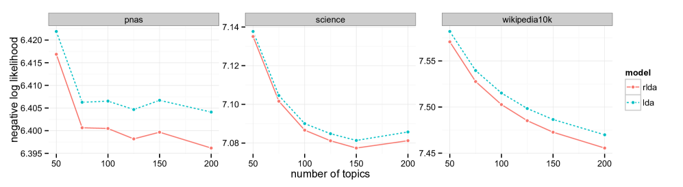
Figure 7: Predictive negative log likelihood on test data. The lower the better. The robust model (rlda) also performs better over a range of topics.

6 Summary

We developed a general method for robust Bayesian modeling. Investigators can create a robust model from a standard Bayesian model by localizing the global variables and then fitting the resulting hyperparameters with empirical Bayes; we described a variational EM algorithm for fitting the model. We demonstrated our approach on generalized linear models and topic models.

David M. Blei is supported by NSF BIGDATA NSF IIS-1247664, NSF NEURO NSF IIS-1009542, ONR N00014-11-1-0651, DARPA FA8750-14-2-0009, Facebook, Adobe, Amazon, the Sloan Foundation, and the John Templeton Foundation. The authors thank Rajesh Ranganath and Yixin Wang for helpful discussions about this work.

References

- Ahn et al. (2012) Ahn, S., Korattikara, A., and Welling, M. (2012). “Bayesian posterior sampling via stochastic gradient Fisher scoring.” arXiv preprint arXiv:1206.6380.
- Airoldi (2007) Airoldi, E. (2007). “Bayesian Mixed-Membership Models of Complex and Evolving Networks.” Ph.D. thesis, Carnegie Mellon University.
- Airoldi et al. (2007) Airoldi, E., Blei, D., Fienberg, S., and Xing, E. (2007). “Combining Stochastic Block Models and Mixed Membership for Statistical Network Analysis.” In Statistical Network Analysis: Models, Issues and New Directions, Lecture Notes in Computer Science, 57–74. Springer-Verlag.
- Airoldi et al. (2009) — (2009). “Mixed Membership Stochastic Blockmodels.” In Neural Information Processing Systems.
- Antoniak (1974) Antoniak, C. (1974). “Mixtures of Dirichlet processes with applications to Bayesian nonparametric problems.” The Annals of Statistics, 2(6): 1152–1174.
- Asuncion et al. (2009) Asuncion, A., Welling, M., Smyth, P., and Teh, Y. (2009). “On Smoothing and Inference for Topic Models.” In Uncertainty in Artificial Intelligence.
- Attias (2000) Attias, H. (2000). “A variational Bayesian framework for graphical models.” In Advances in Neural Information Processing Systems.
- Bernardo and Smith (1994) Bernardo, J. and Smith, A. (1994). Bayesian theory. Chichester: John Wiley & Sons Ltd.
- Bickel and Doksum (2007) Bickel, P. and Doksum, K. (2007). Mathematical Statistics: Basic Ideas and Selected Topics, volume 1. Upper Saddle River, NJ: Pearson Prentice Hall, 2nd edition.
- Bishop (2006) Bishop, C. (2006). Pattern Recognition and Machine Learning. Springer New York.
- Blei (2012) Blei, D. (2012). “Probabilistic Topic Models.” Communications of the ACM, 55(4): 77–84.
- Blei and Lafferty (2007) Blei, D. and Lafferty, J. (2007). “A Correlated Topic Model of Science.” Annals of Applied Statistics, 1(1): 17–35.
- Blei et al. (2003) Blei, D., Ng, A., and Jordan, M. (2003). “Latent Dirichlet Allocation.” Journal of Machine Learning Research, 3: 993–1022.
- Box (1976) Box, G. (1976). “Science and Statistics.” Journal of the American Statistical Association, 71(356): 791–799.
- Box (1980) — (1980). “Sampling and Bayes’ Inference in Scientific Modeling and Robustness.” Journal of the Royal Statistical Society, Series A, 143(4): 383–430.
- Cameron and Trivedi (2013) Cameron, A. C. and Trivedi, P. K. (2013). Regression analysis of count data, volume 53. Cambridge university press.
- Carlin and Louis (2000a) Carlin, B. and Louis, T. (2000a). Bayes and Empirical Bayes Methods for Data Analysis, 2nd Edition. Chapman & Hall/CRC.
- Carlin and Louis (2000b) — (2000b). “Empirical Bayes: Past, present and future.” Journal of the American Statistical Association, 95(452): 1286–1289.
-
Copas (1969)
Copas, J. B. (1969).
“Compound Decisions and Empirical Bayes.”
Journal of the Royal Statistical Society. Series B
(Methodological), 31(3): pp. 397–425.
URL http://www.jstor.org/stable/2984345 - Corduneanu and Bishop (2001) Corduneanu, A. and Bishop, C. (2001). “Variational Bayesian Model Selection for Mixture Distributions.” In International Conference on Artifical Intelligence and Statistics.
- Dempster et al. (1977) Dempster, A., Laird, N., and Rubin, D. (1977). “Maximum likelihood from incomplete data via the EM algorithm.” Journal of the Royal Statistical Society, Series B, 39: 1–38.
- Diaconis and Ylvisaker (1979) Diaconis, P. and Ylvisaker, D. (1979). “Conjugate Priors for Expontial Families.” The Annals of Statistics, 7(2): 269–281.
- Doyle and Elkan (2009) Doyle, G. and Elkan, C. (2009). “Accounting for burstiness in topic models.” In Proceedings of the 26th Annual International Conference on Machine Learning, ICML ’09, 281–288. New York, NY, USA: ACM.
- Efron (1996) Efron, B. (1996). “Empirical Bayes methods for Combining Likelihoods.” Journal of the American Statistical Association, 91(434): 538–550.
- Efron (2010) — (2010). Large-scale inference: empirical Bayes methods for estimation, testing, and prediction, volume 1. Cambridge University Press.
- Efron and Morris (1973) Efron, B. and Morris, C. (1973). “Combining Possibly Related Estimation Problems.” Journal of the Royal Statistical Society, Series B, 35(3): 379–421.
- Efron and Morris (1975) — (1975). “Data analysis using Stein’s estimator and its generalizations.” Journal of the American Statistical Association, 70(350): 311–319.
- Erosheva et al. (2007) Erosheva, E., Fienberg, S., and Joutard, C. (2007). “Describing Disability Through Individual-Level Mixture Models for Multivariate Binary Data.” Annals of Applied Statistics.
- Fei-Fei and Perona (2005) Fei-Fei, L. and Perona, P. (2005). “A Bayesian Hierarchical Model for Learning Natural Scene Categories.” IEEE Computer Vision and Pattern Recognition, 524–531.
- Feng et al. (2014) Feng, J., Xu, H., Mannor, S., and Yan, S. (2014). “Robust Logistic Regression and Classification.” In Advances in Neural Information Processing Systems, 253–261.
- Fernández and Steel (1999) Fernández, C. and Steel, M. F. (1999). “Multivariate Student-t regression models: Pitfalls and inference.” Biometrika, 86(1): 153–167.
- Fine et al. (1998) Fine, S., Singer, Y., and Tishby, N. (1998). “The Hierarchical Hidden Markov Model: Analysis and Applications.” Machine Learning, 32: 41–62.
- Fox et al. (2011) Fox, E., Sudderth, E., Jordan, M., and Willsky, A. (2011). “A Sticky HDP-HMM with Application to Speaker Diarization.” Annals of Applied Statistics, 5(2A): 1020–1056.
- Geisser and Eddy (1979) Geisser, S. and Eddy, W. F. (1979). “A predictive approach to model selection.” Journal of the American Statistical Association, 74(365): 153–160.
- Gelman et al. (2003) Gelman, A., Carlin, J., Stern, H., and Rubin, D. (2003). Bayesian Data Analysis, Second Edition. London: Chapman & Hall, 2nd edition.
- Gelman et al. (1996) Gelman, A., Meng, X., and Stern, H. (1996). “Posterior Predictive Assessment of Model Fitness Via Realized Discrepancies.” Statistica Sinica, 6: 733–807.
- Ghahramani and Beal (2000) Ghahramani, Z. and Beal, M. J. (2000). “Variational Inference for Bayesian Mixtures of Factor Analysers.” In NIPS.
- Grimmer (2009) Grimmer (2009). “A Bayesian Hierarchical Topic Model for Political Texts: Measuring Expressed Agendas in Senate Press Releases.”
- Hoffman et al. (2013) Hoffman, M., Blei, D., Wang, C., and Paisley, J. (2013). “Stochastic Variational Inference.” Journal of Machine Learning Research, 14(1303–1347).
- Hoffman and Gelman (2014) Hoffman, M. D. and Gelman, A. (2014). “The No-U-Turn Sampler: Adaptively Setting Path Lengths in Hamiltonian Monte Carlo.” Journal of Machine Learning Research, 15(Apr): 1593–1623.
- Huber and Ronchetti (2009) Huber, P. and Ronchetti, E. (2009). Robust Statistics. Wiley, 2nd edition.
- Huber (1964) Huber, P. J. (1964). “Robust Estimation of a Location Parameter.” The Annals of Mathematical Statistics, 35(1): 73–101.
- Jordan et al. (1999) Jordan, M., Ghahramani, Z., Jaakkola, T., and Saul, L. (1999). “Introduction to Variational Methods for Graphical Models.” Machine Learning, 37: 183–233.
- Jorgensen (1987) Jorgensen, B. (1987). “Exponential dispersion models.” Journal of the Royal Statistical Society. Series B (Methodological), 127–162.
- Kalman (1960) Kalman, R. (1960). “A New Approach to Linear Filtering and Prediction Problems A New Approach to Linear Filtering and Prediction Problems,”.” Transaction of the AMSE: Journal of Basic Engineering, 82: 35–45.
- Kass and Steffey (1989) Kass, R. and Steffey, D. (1989). “Approximate Bayesian inference in conditionally independent hierarchical models (parametric empirical Bayes models).” Journal of the American Statistical Association, 84(407): 717–726.
- Lange et al. (1989) Lange, K., Little, R., and Taylor, J. (1989). “Robust Statistical Modeling Using the t Distribution.” Journal of the American Statistical Association, 84(408): 881.
- Madsen et al. (2005) Madsen, R. E., Kauchak, D., and Elkan, C. (2005). “Modeling word burstiness using the Dirichlet distribution.” In Proceedings of the 22nd international conference on Machine learning, 545–552. ACM.
- Maritz and Lwin (1989) Maritz, J. and Lwin, T. (1989). Empirical Bayes methods. Monographs on Statistics and Applied Probability. London: Chapman & Hall.
- McCullagh and Nelder (1989) McCullagh, P. and Nelder, J. (1989). Generalized Linear Models. London: Chapman and Hall.
- McLachlan and Peel (2000) McLachlan, G. and Peel, D. (2000). Finite mixture models. Wiley-Interscience.
- Morris (1983) Morris, C. (1983). “Parametric empirical Bayes inference: Theory and applications.” Journal of the American Statistical Association, 78(381): 47–65.
- Murphy (2013) Murphy, K. (2013). Machine Learning: A Probabilistic Approach. MIT Press.
- Paisley and Carin (2009) Paisley, B. and Carin, L. (2009). “Nonparametric Factor Analysis with Beta Process Priors.” In International Conference on Machine Learning.
- Peel and McLachlan (2000) Peel, D. and McLachlan, G. J. (2000). “Robust mixture modelling using the t distribution.” Statistics and Computing, 10(4): 339–348.
- Pregibon (1982) Pregibon, D. (1982). “Resistant fits for some commonly used logistic models with medical applications.” Biometrics, 485–498.
- Pritchard et al. (2000) Pritchard, J. K., Stephens, M., and Donnelly, P. (2000). “Inference of population structure using multilocus genotype data.” Genetics, 155(2): 945–959.
- Rabiner (1989) Rabiner, L. R. (1989). “A tutorial on hidden Markov models and selected applications in speech recognition.” Proceedings of the IEEE, 77: 257–286.
- Ranganath et al. (2014) Ranganath, R., Gerrish, S., and Blei, D. (2014). “Black box variational inference.” In Artificial Intelligence and Statistics.
- Robbins (1964) Robbins, H. (1964). “The empirical Bayes approach to statistical decision problems.” The Annals of Mathematical Statistics, 1–20.
- Robbins (1980) — (1980). “An empirical Bayes estimation problem.” Proceedings of the National Academy of Sciences, 77(12): 6988.
- Rubin (1984) Rubin, D. (1984). “Bayesianly Justifiable and Relevant Frequency Calculations for the Applied Statistician.” The Annals of Statistics, 12(4): 1151–1172.
- Salakhutdinov and Mnih (2008) Salakhutdinov, R. and Mnih, A. (2008). “Probabilistic matrix factorization.” In Neural Information Processing Systems.
- She and Owen (2011) She, Y. and Owen, A. (2011). “Outlier detection using nonconvex penalized regression.” Journal of the American Statistical Association, 106(494).
- Stefanski et al. (1986) Stefanski, L. A., Carroll, R. J., and Ruppert, D. (1986). “Optimally hounded score functions for generalized linear models with applications to logistic regression.” Biometrika, 73(2): 413–424.
- Svensén and Bishop (2005) Svensén, M. and Bishop, C. M. (2005). “Robust Bayesian mixture modelling.” Neurocomput., 64: 235–252.
- Teh et al. (2006) Teh, Y., Jordan, M., Beal, M., and Blei, D. (2006). “Hierarchical Dirichlet processes.” Journal of the American Statistical Association, 101(476): 1566–1581.
-
Teh (2006)
Teh, Y. W. (2006).
“A Hierarchical Bayesian Language Model based on
Pitman-Yor Processes.”
In Proceedings of the 21st International Conference on
Computational Linguistics and 44th Annual Meeting of the Association for
Computational Linguistics, 985–992.
URL http://www.aclweb.org/anthology/P/P06/P06-1124 - Tibshirani and Manning (2013) Tibshirani, J. and Manning, C. D. (2013). “Robust Logistic Regression using Shift Parameters.” CoRR, abs/1305.4987.
-
Venables and Ripley (2002)
Venables, W. N. and Ripley, B. D. (2002).
Modern Applied Statistics with S.
New York: Springer, fourth edition.
ISBN 0-387-95457-0.
URL http://www.stats.ox.ac.uk/pub/MASS4 - Wainwright and Jordan (2008) Wainwright, M. and Jordan, M. (2008). “Graphical models, exponential families, and variational inference.” Foundations and Trends in Machine Learning, 1(1–2): 1–305.
- Wang and Blei (2013) Wang, C. and Blei, D. M. (2013). “Variational inference in nonconjugate models.” The Journal of Machine Learning Research, 14(1): 1005–1031.
- Wang et al. (2011) Wang, C., Paisley, J., and Blei, D. (2011). “Online Variational Inference for the Hierarchical Dirichlet Process.” In International Conference on Artificial Intelligence and Statistics.
- Welling and Teh (2011) Welling, M. and Teh, Y. W. (2011). “Bayesian learning via stochastic gradient Langevin dynamics.” In Proceedings of the 28th International Conference on Machine Learning (ICML-11), 681–688.
- Wood et al. (2014) Wood, F., van de Meent, J. W., and Mansinghka, V. (2014). “A New Approach to Probabilistic Programming Inference.” In Artificial Intelligence and Statistics, 1024–1032.
- Xing et al. (2013) Xing, E. P., Ho, Q., Dai, W., Kim, J. K., Wei, J., Lee, S., Zheng, X., Xie, P., Kumar, A., and Yu, Y. (2013). “Petuum: A New Platform for Distributed Machine Learning on Big Data.” arXiv preprint arXiv:1312.7651.