Using RIXS to uncover elementary charge and spin excitations in correlated materials

Abstract

Despite significant progress in resonant inelastic x-ray scattering (RIXS) experiments on cuprates at the Cu $L$-edge, a theoretical understanding of the cross-section remains incomplete in terms of elementary excitations and the connection to both charge and spin structure factors. Here we use state-of-the-art, unbiased numerical calculations to study the low energy excitations probed by RIXS in undoped and doped Hubbard model relevant to the cuprates. The results highlight the importance of scattering geometry, in particular both the incident and scattered x-ray photon polarization, and demonstrate that on a qualitative level the RIXS spectral shape in the cross-polarized channel approximates that of the spin dynamical structure factor. However, in the parallel-polarized channel the complexity of the RIXS process beyond a simple two-particle response complicates the analysis, and demonstrates that approximations and expansions which attempt to relate RIXS to less complex correlation functions can not reproduce the full diversity of RIXS spectral features.

I Introduction

Resonant inelastic x-ray scattering (RIXS) is an experimental technique in which the transferred energy, momentum and polarization associated with incident and scattered x-ray photons can be measured and analyzed to reveal information about the elementary excitations of a system Ament2011 . In recent years RIXS has attracted considerable attention and positioned itself as a primary experimental technique to probe the excitations in correlated materials, especially transition-metal oxides Schlappa2009 ; Braicovich2009 ; Guarise2010 ; Braicovich2010 ; Schlappa2012 ; Tacon2011 ; Dean2013a ; Dean2013b ; Dean2013c ; Tacon2013 ; Ishii2014 ; Lee2014 ; Dean2014 ; Guarise2014 ; Minola2015 ; Wakimoto2015 . RIXS possesses atomic sensitivity with incoming photons resonantly tuned to a specific atomic absorption edge, making it a particularly unique and powerful tool for characterizing excitations across the Brillouin zone in these materials.

The direct RIXS process consists of two dipole transitions, as shown schematically in Fig. 1 for the Cu L-edge. In the first step an incoming photon excites the ground state by promoting an electron from a filled core shell (Cu $2p$) into the valence shell (Cu $3d$). An intermediate state manifold forms following the charge and spin shake-up which accompany the introduction of a local core-hole potential and this new carrier in the valence shell. In the second step an electron from the valence shell, possessing appropriate atomic character, fills the core-hole, accompanied by an outgoing photon, which leaves the system in an excited final state.

Due to the complexity of this process and the presence of the intermediate state, an interpretation of RIXS spectra has been hindered by an incomplete understanding of how it may be related to other, more fundamental, response functions governing spin, charge, lattice and orbital excitations. In addition, it is well known that polarization plays a key role in understanding selective excitations in Raman spectroscopy Devereaux2007 , but a full polarization analysis involving both incident and scattered x-rays has become possible only now in experiment and only shown theoretically to be important for spin-flip excitations Jia2014 . One would expect that a more complete understanding, at a fundamental level, could be obtained by analyzing the full theoretical RIXS cross-section, accounting for the influence of both the incident and scattered light polarization for a given experimental scattering geometry.

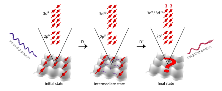
Figure 1: A schematic which illustrates the RIXS process at the Cu $L$-edge appropriate for cuprates.

To better understand the RIXS cross-section from a theoretical perspective, here we will explore a rather general question: what low energy excitations are measured by RIXS, particularly in cuprates at the Cu $L$-edge? There certainly are a number of ways to address this question analytically and numerically. Here, our interest is confined to the low energy excitations which involve spin and/or charge degrees of freedom, neglecting both lattice and higher energy orbital or charge transfer excitations in this work. Our aim will be to qualitatively understand which excitations are encoded in the RIXS cross-section, and any connections to both spin and charge dynamical structure factors, under different scattering conditions; and we will quantitatively compare numerical estimates of the full RIXS cross-section with various approximations to tease out this information.

Naively, one may expect the Cu $L$-edge RIXS cross-section to be the resonant analog of the hard x-ray non-resonant IXS, Jia2012 ; Wang2014 whose response is the charge dynamical structure factor. It then may seem counterintuitive that RIXS at the Cu $L$-edge rose to prominence for the successful empirical measurement of the spin (magnon) dispersion in undoped cuprates, making it a complementary experimental probe to the well-established inelastic neutron scattering Braicovich2010 ; Guarise2010 . With theoretical support Ament2009 ; Jia2014 , experiments on doped cuprates proved sensitive to magnetic excitations, with a similar cross-section to the spin dynamical structure factor, regardless of doping level Tacon2011 ; Dean2013a ; Dean2013b ; Dean2013c ; Tacon2013 ; Ishii2014 ; Lee2014 ; Dean2014 ; Guarise2014 ; Minola2015 ; Wakimoto2015 . These observations were interpreted in terms of persistent magnetic excitations up to an unexpectedly high doping level. However, this semi-empirical connection to the spin dynamical structure factor has been based primarily on approximate theoretical and numerical treatments for the full RIXS cross-section. The fast collision approximation Luo1993 ; Groot1998 ; Veenendaal2006 and the effective operator approach Haverkort2010 suggested that only single magnon excitations or $S(\mathbf{q},\omega)$ should be measured by RIXS at the Cu $L$-edge Ament2009 ; Haverkort2010 ; Marra2012 . More sophisticated treatments – the ultrashort core-hole lifetime (UCL) expansion Ament2007 ; Bisogni2012a ; Bisogni2012b and the UCL-inspired ansatz Igarashi2012a – highlighted that RIXS should be sensitive also to bimagnon excitations. A further extension of UCL also pointed out the importance of three-magnon excitations Ament2010 . However, these studies made no explicit comparison between the approximations and the full RIXS cross-section, nor have they concentrated on the sensitivity of RIXS to the charge dynamical structure factor.

Perhaps more importantly, these approximations suffer from several severe limitations. First, the fast collision approximation (or the effective operator approach) Ament2009 ; Haverkort2010 ; Marra2012 relies on an estimation of the dynamics only at the site where the core-hole has been created in the intermediate state. However, the intermediate state is drawn from a manifold of states, which differ from the ground state not only locally, at the site where a core-hole is created, but also on neighboring sites due to hopping or spin exchange associated with the dynamical screening process. As a result, and especially upon doping, this approximation fails to capture key elements of the full RIXS process. Second, the UCL approximation relies on the assumption that the energies of the intermediate state manifold are much smaller than the inverse core-hole lifetime $\Gamma$, which allows an approximation based on only the first few (two) terms in the UCL Taylor-series-like expansion. However, this assumption need not hold, especially in “itinerant”, doped systems where a number of intermediate states may have energies $\propto t\sim\Gamma$, making the UCL a non-convergent approximation.

In this paper we study the low energy excitations of RIXS at the Cu $L$-edge in an unambiguous way by numerically evaluating the cross-section for a two-dimensional Hubbard model comprising “effective” Cu $3d$ orbitals supplemented by local Cu $2p$ core levels. Using exact diagonalization, which previously was applied to the study of paramagnons in cuprates Jia2014 , we compare the exact RIXS cross-sections to approximate cross-sections for the same model using the same method. The intrinsically correlated nature of our Hamiltonian distinguishes this study from the analytically exact RIXS calculations for the case of completely uncorrelated electrons Benjamin2014 . In the next section, we present and compare numerical results for the exact and approximate RIXS cross-sections, and discuss content of the excitations and consequences for experiments. The paper ends with conclusions, and appendices which contain details and longer derivations.

II Numerical results

II.1 Exact RIXS cross-section

The RIXS cross-section at the Cu $L$-edge is Ament2011 ; Marra2012

$$I_{\bf e}({\bf q},\omega)=\sum_{f}\Big{|}\Big{\langle}f\Big{|}O_{{\bf q},{\bf e}}\Big{|}i\Big{\rangle}\Big{|}^{2}\delta(\omega+E_{i}-E_{f}),$$ (1)

where $|i\rangle$ ($|f\rangle$) is the initial (final) state of the system in the RIXS process with energy $E_{i}$ ($E_{f}$), transfered momentum (energy loss) is ${\bf q}\equiv{\bf k}_{i}-{\bf k}_{f}$ ($\omega\equiv{\omega}_{i}-{\omega}_{f}$) where ${\bf q}_{i}$ and ${\bf q}_{f}$ (${\omega}_{i}$ and ${\omega}_{f}$) are the incoming and outgoing photon momentum (energy), and $\mathbf{e}=\mathbf{e}^{i}\cdot(\mathbf{e}^{f})^{\dagger}$ is the tensor that describes the incoming ($i$) and outgoing ($f$) photon polarizations. Here the operator $O_{{\bf q},{\bf e}}=1/\sqrt{N}\sum_{\bf j}e^{i{\bf q\cdot j}}O_{{\bf j},{\bf e}}$ and

$${O}_{{\bf j},{\bf e}}=D_{{\bf j},{\bf e}^{f}}^{\dagger}\frac{1}{\omega_{i}-\mathcal{H}+\imath\Gamma}D_{{\bf j},{\bf e}^{i}},$$ (2)

which describes the evolution of the system in the RIXS experiment from the initial state to the final state via the intermediate states accessible via the core-hole to valence band dipole transitions. $N$ is the number of lattice sites in the system. The dipole transition operator $D_{{\bf j},{\bf e}}=\sum_{\sigma,\alpha,\beta}(A^{\bf e}_{\alpha}p^{\dagger}_{{\bf j}\alpha\sigma}d_{{\bf j}\sigma}+h.c.)$ with $p_{{\bf j}\alpha\sigma}$ ($d_{{\bf j}\sigma}$) annihilates a hole in the $2p$ ($3d$) shell with spin $\sigma$.$A^{\bf e}_{\alpha}$ is the matrix element of the dipole transition between the 2$p_{\alpha}$ orbitals and 3$d_{x^{2}-y^{2}}$ orbital written as $A^{\bf e}_{\alpha}=\langle d_{x^{2}-y^{2},\sigma}|\hat{\epsilon}\cdot\hat{r}|p_{\alpha\sigma}\rangle$ for polarization $\hat{\epsilon}$. $\Gamma$ is the inverse core-hole lifetime. Note that with the exception of the schematic in Fig. 1, “hole notation” has been used throughout the paper, such that the dipole transitions at the Cu $L$-edge correspond to transitions from the initial $3d^{*1}2p^{0}$ state to a $3d^{*0}2p^{1}$ intermediate state, and finally from the intermediate state to the final state configuration. Here $3d^{*}$ corresponds to holes nominally (Zhang-Rice singlets ZRS ) in the single band notation.

Here we use the single-band Hubbard model as it carries the key features of correlated materials in the low energy regime, which are the relevant energy regime for the study of charge and spin excitations for cuprates in RIXS measurements. The single-band results can be applied directly to cuprates and can be generalized to other multi-orbital correlated materials. The Hamiltonian $\mathcal{H}$ defined on a 2D square lattice describes the relevant interactions of the “effective” $3d$ and $2p$ orbitals, consisting of two parts:

$$\mathcal{H} =H+H_{c},$$ (3)

$${{H}} \!=\!-t\!\!\sum_{\langle{\bf i},{\bf j}\rangle,\sigma}d_{{\bf i}\sigma}^{\dagger}d_{{\bf j}\sigma}\!-\!t^{\prime}\!\!\sum_{\langle\langle{\bf i},{\bf j}\rangle\rangle,\sigma}d_{{\bf i}\sigma}^{\dagger}d_{{\bf j}\sigma}\!+\!U\!\sum_{\bf i}n_{{\bf i}\uparrow}^{d}n_{{\bf i}\downarrow}^{d},$$ (4)

$${{H}}_{c} \!=\!(\epsilon^{d}\!-\!\epsilon^{p})\sum_{{\bf i}\alpha\sigma}n_{{\bf i}\alpha\sigma}^{p}+\mathit{U}_{c}\sum_{{\bf i}\alpha\sigma\sigma^{\prime}}n_{{\bf i}\sigma}^{d}n_{{\bf i}\alpha\sigma^{\prime}}^{p}$$

$$+\lambda\sum_{{\bf i}\alpha\alpha^{\prime}\sigma\sigma^{\prime}}p_{{\bf i}\alpha\sigma}^{\dagger}\chi_{\alpha\alpha^{\prime}}^{\sigma\sigma^{\prime}}p_{{\bf i}\alpha^{\prime}\sigma^{\prime}}.$$ (5)

The first part, Eq. (4), is the well-known single-band Hubbard model with the nearest (next-nearest) neighbor hopping $t$ ($t^{\prime}$) and on-site Hubbard repulsion $U$. Here, the operator $d^{\dagger}$ in the single-band Hubbard model creates a “$3d^{*}$” hole, which should be distinguished from the actual Cu $3d_{x^{2}-y^{2}}$ hole in the multiband model. The second part, Eq. (5), describes (i) the energy splitting between the $2p$ and the $3d$ shells through the difference in site energy $\epsilon^{d}\!-\!\epsilon^{p}$, (ii) the repulsion between the $2p$ and the $3d$ holes (the “core-hole potential”) $U_{c}$, and (iii) the spin-orbit coupling in the $2p$ shell $\lambda$ with the matrix elements $\chi_{\alpha\alpha^{\prime}}^{\sigma\sigma^{\prime}}\equiv\langle p_{\alpha\sigma}|\mathbf{l}\cdot\mathbf{s}|p_{\alpha^{\prime}\sigma^{\prime}}\rangle$, where the $\mathbf{l}\cdot\mathbf{s}$ term represents the spin-orbit coupling operator.

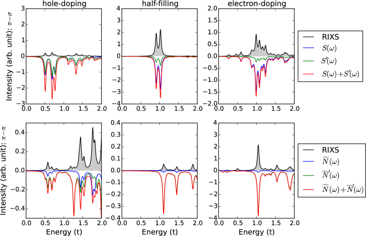
Figure 2: Exact RIXS cross-sections and approximations calculated using exact diagonalization. Top (bottom) panels show spectra for the $\pi-\sigma$ ($\pi-\pi$) polarization geometries. Left, middle, and right panels show RIXS spectra calculated for $n=0.83$ (“hole-doping”), $n=1$ (“half-filling”), and $n=1.17$ (“electron doping”) electron fillings, respectively. The spectra are summed over all momenta along the nodal direction and along the $k_{y}=0$ direction that are accessible in RIXS on a 12-site cluster, weighted with the RIXS form factors, i.e.: $S(\omega)=\sum_{\bf q}|{W}_{\bf\pi\!-\!\sigma}|^{2}S({\bf q},\omega)$, $\tilde{N}(\omega)=\sum_{\bf q}|{W}_{\bf\pi\!-\!\pi}|^{2}\tilde{N}({\bf q},\omega)$ and similarly for $S^{\prime}(\omega)$ and $\tilde{N^{\prime}}(\omega)$. The elastic response has been removed in each panel.

The RIXS cross-section is calculated using exact diagonalization on a 12-site cluster. In this cluster, momentum points (2$\pi$/3,0) and ($\pi$/2, $\pi$/2) are accessible, providing information along both the Brillouin zone axis and diagonal, relevant for RIXS experiments. As the Cu 2p core levels and the spin-orbit coupling are included (which also means that the total spin is not a good quantum number in the intermediate state), the Hilbert space size is $\sim 10^{7}$. Ground state eigenvectors and eigenvalues were obtained using the implicitly restarted Arnoldi method encoded in the Parallel ARPACK Lehoucq1998 libraries. The cross-section itself was obtained using the biconjugate gradient stabilized method Vorst1992 and continued fraction expansion Dagotto1994 . The numerical technique has been applied previously to calculate RIXS at the Cu $K$-edge and $L$-edges Jia2012 ; Jia2014 . Numerical results were obtained for parameters which can relatively well reproduce the low energy physics for cuprates: $\epsilon^{d}-\epsilon^{p}=2325t$ (which gives the typical splitting between the Cu $2p$ and the Cu $3d$ shell of 930 eV if $t=0.4$eV), $U_{c}=4t$, $\lambda=32.5t$, $\Gamma=t$, $U=8t$, $t^{\prime}=-0.3t$. RIXS spectra at half-filling are taken at the Cu $L_{3}$ resonance (i.e. $\omega_{i}\sim\epsilon^{d}\!-\!\epsilon^{p}+E_{L_{3}}$ with $E_{L_{3}}=-\lambda/2$). For doped systems, we investigate at the resonance where the character of the intermediate state is similar to that in the undoped case on the core-hole site. The angle between the incident and the scattered photons is set to $50^{\circ}$, with the scattering plane parallel to $xz$, i.e. perpendicular to the $xy$ plane on which we define the 2D Hubbard Hamiltonian, and the incoming polarization is chosen to be $\pi$. This scattering geometry is consistent with that used most commonly in RIXS measurments for cuprates Dean2013a ; Dean2013b ; Dean2013c ; Ishii2014 ; Lee2014 ; Dean2014 ; Guarise2014 . The relation between polarization and the transferred momenta Veenendaal2006 ; Ament2009 ; Haverkort2010 ; Wohlfeld2013 follows from this scattering geometry: ${\bf e}^{i}=(\sin\theta,0,\cos\theta)$, ${\bf e}^{f}=[-\cos(\theta-40^{\circ}),0,\sin(\theta-40^{\circ})]$ [${\bf e}^{f}=(0,-1,0)$] for outgoing $\pi$ ($\sigma$) polarization, $\theta\in[0^{\circ},130^{\circ}]$, and the angle $\theta$ is related to the transferred momentum via $k_{x}=1.07\pi\sin(\theta-65^{\circ})$. The calculated RIXS spectra will be presented at Figs. 2 - 5. The comparison with the approximated spectra will be presented in Section II C below.

II.2 Approximate cross-section

The approximations follow from integrating out the core hole degrees of freedom using two approaches. We firstly assume that the energy of the incoming photon $\omega_{i}$ is tuned to the main resonance at the Cu $L_{3}$ edge, as dictated by $H_{c}$. This is equivalent to a projection into a subspace with only one $3d^{*}$ hole on the core-hole site in either the initial state $|i\rangle$ or the final state $|f\rangle$. We then perform the UCL approximation by expanding the RIXS operator, Eq. (2), in a power series in $\mathcal{H}/\Gamma$ and only keeping the first two terms. See Appendix A for details. These approximations can be written separately for the two polarization conditions as follows:

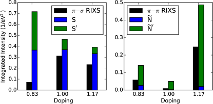
Figure 3: Momentum and energy integrated spectral weightfor full RIXS $\int_{0}^{1.6t}I(\omega){\rm d}\omega$and the various approximations $S=\int_{0}^{1.6t}S(\omega){\rm d}\omega$, $\tilde{N}=\int_{0}^{1.6t}\tilde{N}(\omega){\rm d}\omega$, ${S^{\prime}}=\int_{0}^{1.6t}S^{\prime}(\omega){\rm d}\omega$, $\tilde{N^{\prime}}=\int_{0}^{1.6t}\tilde{N^{\prime}}(\omega){\rm d}\omega$ with $S(\omega),\tilde{N}(\omega),S^{\prime}(\omega),\tilde{N^{\prime}}(\omega)$ defined as in the caption of Fig. 2 RIXS spectra. The $\pi-\sigma$ ($\pi-\pi$) relative polarizations are shown on the left (right) panels, respectively. Note that the spectral weight $\tilde{N}=5\times 10^{-5}(eV)^{-2}$ in the half-filled case and does not appear in the figure.All momenta along the nodal direction and along the $q_{y}=0$ direction accessible on a 12-site cluster are taken into account (elastic response excluded).

$\pi\!-\!\sigma$ RIXS in the UCL approximation:

$$I^{\rm UCL}_{\bf\pi\!-\!\sigma}({\bf q},\omega)\!= |{W}_{\bf\pi\!-\!\sigma}|^{2}\Big{\{}S({\bf q},\omega)+S^{\prime}({\bf q},\omega)\Big{\}},$$ (6)

$$S({\bf q},\omega)\!= \sum_{f}\Big{|}\Big{\langle}f\Big{|}{S}_{\bf q}^{z}\Big{|}i\Big{\rangle}\Big{|}^{2}\delta(\omega\!+\!E_{i}\!-\!E_{f}),$$ (7)

$$S^{\prime}({\bf q},\omega)\!= \frac{z^{2}t^{2}}{N^{2}\Gamma^{2}}\sum_{f}\Big{|}\Big{\langle}f\Big{|}\sum_{{\bf k},{\bf k^{\prime}}}\varepsilon_{-{\bf k^{\prime}}+{\bf k}+{\bf q}}S^{z}_{\bf k^{\prime}}$$

$$\times{d}_{{\bf k},\sigma}^{\dagger}{d}_{-{\bf k^{\prime}}+{\bf k}+{\bf q},\sigma}\Big{|}i\Big{\rangle}\Big{|}^{2}\delta(\omega\!+\!E_{i}\!-\!E_{f}),$$ (8)

where the local RIXS form factor ${W}_{\bf\pi\!-\!\sigma}=-\imath 2\sin\theta/(3\Gamma)$, the spin operator ${S}^{z}_{\bf q}=1/({2\sqrt{N}})\sum_{{\bf k}}({d}_{{\bf k},\uparrow}^{\dagger}{d}_{{\bf q}+{\bf k},\uparrow}-{d}_{{\bf k},\downarrow}^{\dagger}{d}_{{\bf q}+{\bf k},\downarrow})$, $z=4$ is the 2D coordination number, and the 2D structure factor is $\varepsilon_{{\bf k}}=\gamma_{{\bf k}}+t^{\prime}\eta_{{\bf k}}/t$ with $\gamma_{\bf k}=(\cos k_{x}+\cos k_{y})/2$ and $\eta_{\bf k}=\cos k_{x}\cos k_{y}$. The structure factor $\varepsilon_{{\bf k}}$ has $A_{1g}$ symmetry. Note that the first term of the expansion $S({\bf q},\omega)$ has the form of the spin dynamical structure factor, while the second term $S^{\prime}({\bf q},\omega)$ is a rather complicated four particle response which probes spin and charge excitations. The latter corresponds to the 3-spin Greens function (see Appendix B) and to joint spin and charge excitations.

$\pi\!-\!\pi$ RIXS in UCL approximation:

$$I^{\rm UCL}_{\bf\pi\!-\!\pi}({\bf q},\omega)\!= |{W}_{\bf\pi\!-\!\pi}|^{2}\Big{\{}\tilde{N}({\bf q},\omega)+\tilde{N^{\prime}}({\bf q},\omega)\Big{\}},$$ (9)

$$\tilde{N}({\bf q},\omega)\!= \sum_{f}\Big{|}\Big{\langle}f\Big{|}\tilde{n}_{\bf q}\Big{|}i\Big{\rangle}\Big{|}^{2}\delta(\omega\!+\!E_{i}\!-\!E_{f}),$$ (10)

$$\tilde{N^{\prime}}({\bf q},\omega)\!= \frac{z^{2}t^{2}}{N\Gamma^{2}}\sum_{f}\Big{|}\Big{\langle}f\Big{|}\sum_{\bf k}\varepsilon_{{\bf q}+{\bf k}}\tilde{d}_{{\bf k},\sigma}^{\dagger}{d}_{{\bf q}+{\bf k},\sigma}\Big{|}i\Big{\rangle}\Big{|}^{2}$$

$$\times\delta(\omega\!+\!E_{i}\!-\!E_{f}),$$ (11)

where the constrained density operator is $\tilde{{n}}_{\bf i}=\sum_{\sigma}\tilde{d}^{{\dagger}}_{{\bf i}\sigma}\tilde{d}_{{\bf i}\sigma}$ with constrained fermions $\tilde{d}^{{\dagger}}_{{\bf i}\sigma}={d}_{{\bf i}\sigma}^{{\dagger}}(1-n_{{\bf i}\bar{\sigma}})$ and $\tilde{d}_{{\bf i}\sigma}=(1-n_{{\bf i}\bar{\sigma}}){d}_{{\bf i}\sigma}$, and the local RIXS form factor ${W}_{\bf\pi\!-\!\pi}=-2\sin\theta\cos(\theta-40^{\circ})/(3\Gamma)$.

Before evaluating the correlation functions, we want to highlight that none of these approximations give the standard charge dynamical structure factors for the parallel-polarization channel. The first term of the expansion, $\tilde{N}({\bf q},\omega)$, is not the standard charge dynamical structure factor. It represents a more complicated four-particle response function in the original space of unprojected fermions. In the following, it carries information about projected charge excitations, which should in no way be confused with information about the full charge response. That RIXS does not probe the standard charge response stems from the fact that initial states with double occupancy on the core-hole site can not be excited in the RIXS process due to the Pauli principle. The second term $\tilde{N^{\prime}}({\bf q},\omega)$, a complicated four-particle response function as well, corresponds to 2-spin or bimagnon excitations (see Appendix B) and other symmetry projected charge excitations, represented again by a correlator beyond the familiar two-particle charge response.

II.3 Comparing exact and approximate results

In the following, we will present a systematic comparison of the full RIXS spectra with the approximations using the UCL expansion for the two polarization conditions. As a momentum resolved technique, RIXS has the power to measure the dispersion of elementary excitations, which is one of its main advantages compared to traditional optical or Raman scattering, where the momentum transfer is limited to $q\sim 0$. Devereaux2007 However, there are limitations in cluster size, as well as a limited number of poles using a finite-size cluster. Thus, summing over all the accessible momentum points (results as shown in Fig. 2) gives us a complete picture of the energies and the distribution of intensities for the excitations, so that the comparisons to the approximations can be made in a single shot. To better quantify this comparison, we also calculate and compare the total spectral weight carried by the excitations, cf. Fig. 3. Nevertheless, in section II D, we compare exact RIXS cross-sections and approximations at the momentum points (2$\pi$/3,0) and ($\pi$/2, $\pi$/2), and discuss connections to experiments.

The full cross-sections are shown in Fig. 2 for two polarization channels: (i) the cross-polarized channel [$\pi-\sigma$ with $\pi$ ($\sigma$) incoming (outgoing) polarization] and (ii) the parallel-polarized channel [$\pi-\pi$ with $\pi$ ($\pi$) incoming (outgoing) polarization]. For each the spectra are calculated for three different doping levels ($n=0.83$, “hole-doping”, $n=1$, “half-filling”, and $n=1.17$, “electron doping”). The $\pi-\sigma$ RIXS spectra presented here agree with those presented in Ref. [Jia2014, ]. The approximate cross-sections $S(\omega)$ and $S^{\prime}(\omega)$ for cross-polarization and $\tilde{N}(\omega)$ and $\tilde{N}^{\prime}(\omega)$ for parallel-polarization are also shown in Fig. 2. The results for both full and approximated RIXS are shown for a Lorentzian broadening with half width at half maximum (HWHM) = $0.025t$ for the energy transfer. Note that the spectra in Fig. 2 correspond to a momentum summation over all points accessible in the 12-site cluster, to provide a holistic picture of the character of excitations probed by RIXS and the utility of various approximations (see Fig. 2 caption for details).

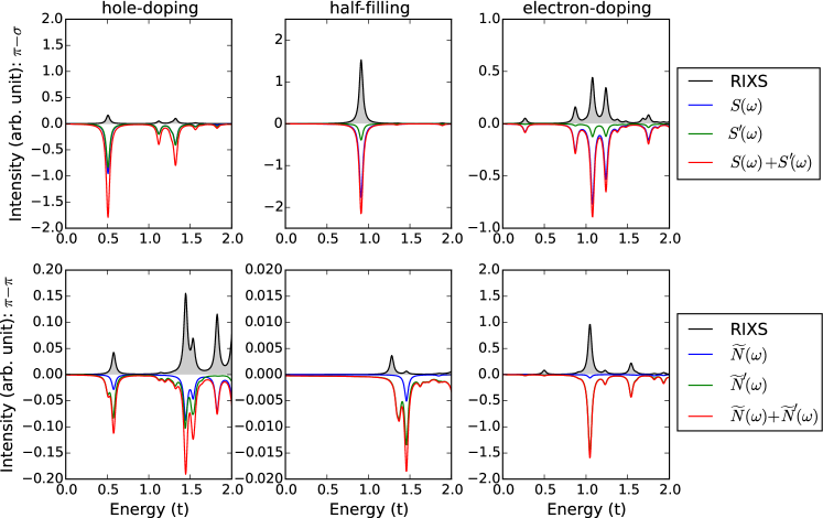
Figure 4: Cross-sections at ${\bf q}=(2\pi/3,0)$ with the elastic response removed.Top (bottom) panels show spectra for the $\pi-\sigma$ ($\pi-\pi$) polarization. Left, middle, and right panels show RIXS spectra for $n=0.83$, $n=1$, and $n=1.17$ electron fillings, respectively. The approximate spectra are weighted with the RIXS form factors, i.e.$S({\bf q},\omega)\rightarrow|{W}_{\bf\pi\!-\!\sigma}|^{2}S({\bf q},\omega)$, $\tilde{N}({\bf q},\omega)\rightarrow|{W}_{\bf\pi\!-\!\pi}|^{2}\tilde{N}({\bf q},\omega)$ and similarly for $S^{\prime}({\bf q},\omega)$ and $\tilde{N^{\prime}}({\bf q},\omega)$.

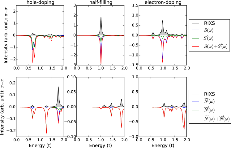
Figure 5: Cross-sections at ${\bf q}=(\pi/2,\pi/2)$ point with the elastic response removed.Top (bottom) panels show spectra for the $\pi-\sigma$ ($\pi-\pi$) polarization. Left, middle, and right panels show RIXS spectra calculated for $n=0.83$, $n=1$, and $n=1.17$ electron fillings, respectively. The approximate spectra are weighted with the RIXS form factors, i.e.$S({\bf q},\omega)\rightarrow|{W}_{\bf\pi\!-\!\sigma}|^{2}S({\bf q},\omega)$, $\tilde{N}({\bf q},\omega)\rightarrow|{W}_{\bf\pi\!-\!\pi}|^{2}\tilde{N}({\bf q},\omega)$ and similarly for $S^{\prime}({\bf q},\omega)$ and $\tilde{N^{\prime}}({\bf q},\omega)$.

First note the results in the cross-polarized channel (the $\pi-\sigma$ channel). On a qualitative level, the line shape of the full RIXS cross-section can be reproduced well by the spin dynamical structure factor $S({\bf q},\omega)$ (the first term of the UCL approximation). This is true at half-filling, where all charge excitations have been gapped-out, while in either the electron- or hole-doped cases one can observe some relatively small discrepancies between the two spectra. When adding higher order terms from the effective expansion, to a large extent this observation remains unchanged since these terms encode similar excitations to $S({\bf q},\omega)$ together with excitations of mixed charge and spin character, as can be seen readily from the form of the operator in Eq. (8).

However, on a quantitative level, this comparison breaks down, with discrepancies in the overall intensity and integrated spectral weight which can become very large (see Fig. 3). While one may have expected that higher order terms in the effective expansion should provide a more satisfactory qualitative and quantitative agreement, these do not help in reducing the differences; on the contrary, these additional terms actually enhance the quantitative mismatch. Note that the first two terms of the UCL expansion suggest larger spectral weight for the hole-doped case compared to that with electron-doping, in contrast to the behavior for the RIXS cross-section. This suggests that the differences cannot be attributed to a simple rescaling factor.

The quantitative mismatch between RIXS at the Cu $L$-edge and the approximations highlights the role that the intermediate state wavefunction plays in the RIXS spectra, just as in the case for RIXS at the Cu $K$-edge. Jia2012 RIXS is an intrinsic four-particle process, where the wavefunction overlap between the ground state and intermediate states, and between intermediate states and final states both play an important role. Neglecting the intermediate state wavefunction might still provide information on the fundamental excitation energies, but unfortunately it cannot provide reasonable spectral weights on a quantitative level. This mismatch also illustrates the failure of these approximations. That being said, both numerically and empirically, in the cross-polarized scattering geometry the RIXS cross-section qualitatively corresponds to the spin dynamical structure factor which encodes information about spin excitations at the two particle level, which underscores RIXS utility as a complementary probe to inelastic neutron scattering.

An altogether different situation arises in the parallel-polarized channel (the $\pi-\pi$ channel). While a comparison between the RIXS spectrum and the “projected” charge excitations produces a modest qualitative agreement between the line shapes, both missing peaks as well as significant differences in the spectral weights undermine any quantitative value in this comparison. The addition of the higher order terms seems to be needed for a better qualitative comparison of the line shapes although both terms support similar spectral excitations based on the form of the operators in Eqs. (10) and (11) and a spectral weight analysis precludes any quantitative agreement. In both cases, while the RIXS spectral lineshape may be approximated by the two expansion terms, neither provides a faithful representation for the proper two-particle charge response encoded in the simple dynamical structure factor, placing statements about the true charge excitation character of the RIXS cross-section on less solid footing.

II.4 Consequences for RIXS experiments

The preceding section presented a comparison between cross-sections integrated in momentum, as well as energy for a total spectral weight analysis. In this section we show spectra at two particular momenta: ${\bf q}=(2\pi/3,0)$ and ${\bf q}=(\pi/2,\pi/2)$ (see Fig. 4 and Fig. 5) to underscore those results, shown in a context amenable to experiment. When doped, the Hubbard model, and by extension cuprates, will possess spin and charge excitations in a similar low energy regime which will appear, either directly or in a more complicated way reflecting the complexity of the cross-section, in the RIXS spectrum for the crossed- and parallel-polarization channels, respectively. Thus, to satisfactorily distinguish between the magnetic and charge channel, or two-spin excitations, one must perform measurements which can discriminate the outgoing polarizations. Unfortunately, to this point RIXS experiments have been unable to fully distinguish between the cross-polarized and parallel-polarized channels, making some statements with the help of a careful analysis of experimental RIXS scattering geometry. The newly constructed, state-of-the-art RIXS end-station at ESRF now provides an opportunity to perform such measurements (cf. Ref. [Minola2015, ]); and other end-stations (currently operational or to be commissioned in the coming years) also would allow for the differentiation between the crossed- and parallel-polarized channels.

Even with outgoing polarization discrimination, in either the crossed- or parallel-polarized channels one needs to carefully invoke either $S(\mathbf{q},\omega)$ or $\tilde{N}(\mathbf{q},\omega)$ as approximations for the full RIXS cross-section. This especially may be true when analyzing RIXS spectral weights as a function of doping. None of these approximations address intermediate state effects, or equivalently differences in the cross-section with changes in the incoming photon energy. Jia2012 Thus, to address the full resonant profile one always needs to calculate the full RIXS cross-section.

III Conclusions

Overall, one must carefully apply approximations for calculating the RIXS cross-section. The nonlocal character of the intermediate state can become particularly important in correlated ground states with longer range entanglement. Therefore, we suggest the full RIXS simulations will be needed to verify the character of excitations.

In the cross-polarized channel, we have shown that on a qualitative level Cu $L$-edge RIXS line shapes correspond to the spin dynamical structure factor $S({\bf q},\omega)$, consistent with lowest order approximations as postulated by the fast collision approximation (or the effective operator approach) Ament2009 ; Haverkort2010 ; Marra2012 ; Jia2014 , see Appendix C. As a consequence, we expect that the line shapes reported from cross-polarized RIXS experiments can be reproduced to some extent by theoretical modeling of the spin dynamical structure factors (or empirically through inelastic neutron scattering experiments when also considering differences in the effective matrix elements between the two techniques). However, the detailed analysis in this paper suggests that a quantitative comparison between RIXS and the two-particle spin and charge dynamical structure factors would be impractical. One should not expect a meaningful comparison between different spectral weights obtained from these different techniques, either experimentally or from simulation.

In the parallel-polarized channel, the situation is further complicated by the operator form taken by the approximations themselves. On a qualitative level the primary contributions seem to follow from higher order terms $\tilde{N^{\prime}}({\bf q},\omega)$, with a notable exception at half-filling, see Appendix C. However, any precise quantitative comparison to experiment would require calculating the full RIXS cross-section. At the same time none of the terms in the approximations correspond to proper two-particle charge excitations, but rather inherently reflect the complexity of the RIXS process. Thus, while line shapes in RIXS should closely resemble the line shapes of the (projected) charge excitations, the spectral weights may be quite different, with a more complicated analysis required to tease out the character of various spectral peaks.

Appendix A: Derivation of the UCL approximation for RIXS at the Cu $L$-edge

The UCL approximation should be valid when all the relevant eigenenergies of the intermediate state Hamiltonian $\mathcal{H}$ are much smaller than the inverse core-hole lifetime $\Gamma$. We use the following spectral decomposition

$$\frac{1}{\omega_{i}-\mathcal{H}+i\Gamma}=\sum_{|N\rangle}|N\rangle\langle N|\frac{1}{\omega_{i}-{\mathcal{E}_{N}}+i\Gamma},$$ (12)

where $\{|N\rangle\}$ are eigenstates of $\mathcal{H}$ with energy $\{\mathcal{E}_{N}\}$. We are interested in RIXS at the resonant edge between the $2p^{0}3d^{*1}$ initial configuration and the $2p^{1}3d^{*0}$ intermediate state configuration. (All expressions are presented in hole language.) This means that we need to exclude all intermediate states $|N\rangle$ which contain one hole in the $d$ orbital on site ${\bf j}$, i.e. on the core-hole site. We add a projection operator $\tilde{P}_{\bf j}$ and rewrite the above expression as

$$\sum_{|N\rangle}|N\rangle\langle N|\frac{1}{\omega_{i}-{\mathcal{E}_{N}}+i\Gamma}\rightarrow\sum_{|N\rangle}\tilde{P}_{\bf j}|N\rangle\langle N|\tilde{P}_{\bf j}\frac{1}{\omega_{i}-{\mathcal{E}_{N}}+i\Gamma}.$$ (13)

We define the following Hamiltonians $\bar{H}=H+\mathit{U}_{c}\sum_{{\bf i}\alpha\sigma\sigma^{\prime}}n_{{\bf i}\sigma}^{d}n_{{\bf i}\alpha\sigma^{\prime}}^{p}$ and $\bar{H}_{c}=H_{c}-\mathit{U}_{c}\sum_{{\bf i}\alpha\sigma\sigma^{\prime}}n_{{\bf i}\sigma}^{d}n_{{\bf i}\alpha\sigma^{\prime}}^{p}$. Note that $\bar{H}$ and $\bar{H}_{c}$ commute (and $\mathcal{H}=\bar{H}+\bar{H}_{c}$), since the intermediate states of RIXS are such that they always contain either a hole in the $2p$ shell or in the $3d$ shell (guaranteed by the projection operators $\tilde{P}_{\bf j}$). Then we obtain:

$$|N\rangle=|n\rangle|n_{c}\rangle\quad\mathcal{E}_{N}=\varepsilon_{n}+\varepsilon_{n_{c}},$$ (14)

where $|n\rangle$ are eigenstates of $\bar{H}$ with energy $\varepsilon_{n}$, $|n_{c}\rangle$ are eigenstates of $\bar{H}_{c}$ with energy $\varepsilon_{n_{c}}$. Consequently we can write

$$\frac{1}{\omega_{i}-\mathcal{H}+i\Gamma}= \sum_{|n\rangle,|n_{c}\rangle}\tilde{P}_{\bf j}|n\rangle\langle n|n_{c}\rangle\langle n_{c}|\tilde{P}_{\bf j}$$

$$\times\frac{1}{\omega_{i}-\varepsilon_{n}-\varepsilon_{n_{c}}+i\Gamma}.$$ (15)

Note that with a single hole in the $p$ shell, there are just two eigenstates of $\bar{H}_{c}$: $n_{c}\in{|L_{2}\rangle,|L_{3}\rangle}$ with energies ${\varepsilon_{L_{2}},\varepsilon_{L_{3}}}$. They correspond to the two ‘$j$’ eigenstates $j=1/2$ and $j=3/2$, respectively, split by the spin-orbit coupling $\propto\lambda$. (We note that $j$ represents the angular momentum and $\mathbf{j}$ represents site $\mathbf{j}$ on the cluster.) This implies

$$\frac{1}{\omega_{i}-\mathcal{H}+i\Gamma}= \sum_{|n\rangle}\tilde{P}_{\bf j}|n\rangle\langle n|L_{2}\rangle\langle L_{2}|\tilde{P}_{\bf j}\frac{1}{\omega_{i}-\varepsilon_{n}-\varepsilon_{L_{2}}+i\Gamma}$$

$$+ \sum_{|n\rangle}\tilde{P}_{\bf j}|n\rangle\langle n|L_{3}\rangle\langle L_{3}|\tilde{P}_{\bf j}\frac{1}{\omega_{i}-\varepsilon_{n}-\varepsilon_{L_{3}}+i\Gamma}.$$ (16)

Resonance approximation We assume that the incoming x-ray photons are tuned to the $L_{3}$ resonance, i.e. $\omega_{i}\simeq\varepsilon_{L_{3}}$. Since $\lambda\gg\Gamma$ (and all eigenenergies $\varepsilon_{n}\ll\lambda$), we can neglect the contribution from the $L_{2}$ resonance and obtain

$$\frac{1}{\omega_{i}-\mathcal{H}+i\Gamma}=\sum_{|n\rangle}\tilde{P}_{\bf j}|n\rangle\langle n|L_{3}\rangle\langle L_{3}|\tilde{P}_{\bf j}\frac{1}{-\varepsilon_{n}+i\Gamma}.$$ (17)

UCL expansion We adopt the UCL expansion Brink2006 ; Forte2008 ; Ament2010 for Cu $L$-edge RIXS to obtain

$$\frac{1}{\omega_{i}-\mathcal{H}+i\Gamma}=\tilde{P}_{\bf j}|L_{3}\rangle\langle L_{3}|\sum_{l=0}^{+\infty}\frac{{\bar{H}}^{l}}{(i\Gamma)^{l+1}}\tilde{P}_{\bf j}.$$ (18)

This means that the RIXS operator can be rewritten as

$${O}_{{\bf j},{\bf e}}=\frac{1}{i\Gamma}D_{{\bf j},{\bf e}^{f}}^{\dagger}\tilde{P}_{\bf j}|L_{3}\rangle\langle L_{3}|\sum_{l=0}^{+\infty}\frac{{\bar{H}}^{l}}{(i\Gamma)^{l}}\tilde{P}_{\bf j}D_{{\bf j},{\bf e}^{i}}.$$ (19)

Second order UCL approximation Keeping only terms with $l=0$ and $l=1$ gives

$${O}_{{\bf j},{\bf e}}= {O}^{(1)}_{{\bf j},{\bf e}}+{O}^{(2)}_{{\bf j},{\bf e}}$$ (20)

$${O}^{(1)}_{{\bf j},{\bf e}}= \frac{1}{i\Gamma}D_{{\bf j},{\bf e}^{f}}^{\dagger}\tilde{P}_{\bf j}|L_{3}\rangle\langle L_{3}|\tilde{P}_{\bf j}D_{{\bf j},{\bf e}^{i}}$$

$${O}^{(2)}_{{\bf j},{\bf e}}= \frac{1}{(i\Gamma)^{2}}D_{{\bf j},{\bf e}^{f}}^{\dagger}\tilde{P}_{\bf j}|L_{3}\rangle\langle L_{3}|{\bar{H}}\tilde{P}_{\bf j}D_{{\bf j},{\bf e}^{i}}.$$ (21)

The validity of this approximation has been discussed in detail in the main text of the paper.

Change of projection operators It is convenient to use another operator – $P_{\bf j}$ – which projects to the sector with no doubleoccupancy in the $d$ level on site ${\bf j}$, i.e. where the core-hole is created. This gives

$$\tilde{P}_{\bf j}D_{{\bf j},{\bf e}^{i}}=D_{{\bf j},{\bf e}^{i}}{P}_{\bf j}.$$ (22)

A similar expression holds also for the $D^{{\dagger}}_{{\bf j},{\bf e}^{f}}$ dipole operator.

The $l=1$ term Next we evaluate

$$P_{\bf j}D_{{\bf j},{\bf e}^{f}}^{\dagger}|L_{3}\rangle\langle L_{3}|{\bar{H}}D_{{\bf j},{\bf e}^{i}}P_{\bf j}|i\rangle.$$ (23)

Since

$$P_{\bf j}D_{{\bf j},{\bf e}^{f}}^{\dagger}|L_{3}\rangle\langle L_{3}|\bar{H}_{\bf mj}D_{{\bf j},{\bf e}^{i}}P_{\bf j}|i\rangle=0$$ (24)

where

$$\bar{H}_{\bf mj}= -t\!\!\sum_{m(j),\sigma}({d}^{\dagger}_{{\bf m}\sigma}{d}_{{\bf j}\sigma}\!+\!h.c.)-t^{\prime}\!\!\sum_{{\bf m}^{\prime}({\bf j}),\sigma}({d}^{\dagger}_{{\bf m}^{\prime}\sigma}{d}_{{\bf j}\sigma}\!+\!h.c.)$$

$$+\mathit{U}_{c}\sum_{\alpha\sigma\sigma^{\prime}}n_{{\bf j}\sigma}^{d}n_{{\bf j}\alpha\sigma^{\prime}}^{p}+\!U\!n_{{\bf j}\uparrow}^{d}n_{{\bf j}\downarrow}^{d}$$ (25)

due to the fact that all terms in the Hamiltonian which contain site j will vanish when “sandwiched”’ between the dipole operators $D$ and evaluated on the initial state $|i\rangle$. Here ${\bf m}({\bf j})$ and ${\bf m}^{\prime}({\bf j})$ are nearest and next nearest neighbors of site ${\bf j}$.

Thus, the following expression holds:

$$P_{\bf j}D_{{\bf j},{\bf e}^{f}}^{\dagger}|L_{3}\rangle\langle L_{3}|{\bar{H}}D_{{\bf j},{\bf e}^{i}}P_{\bf j}|i\rangle=P_{\bf j}D_{{\bf j},{\bf e}^{f}}^{\dagger}|L_{3}\rangle\langle L_{3}|$$

$$\times({\bar{H}}-\bar{H}_{\bf mj})D_{{\bf j},{\bf e}^{i}}P_{\bf j}|i\rangle.$$ (26)

Commuting the Hamiltonian ${\bar{H}}-\bar{H}_{\bf mj}$ (which does not contain operators on site j) with the operator $D_{{\bf j},{\bf e}^{i}}$ and $P_{\bf j}$ to gives

$$P_{\bf j}D_{{\bf j},{\bf e}^{f}}^{\dagger}|L_{3}\rangle\langle L_{3}|{\bar{H}}D_{{\bf j},{\bf e}^{i}}P_{\bf j}|i\rangle=P_{\bf j}D_{{\bf j},{\bf e}^{f}}^{\dagger}|L_{3}\rangle\langle L_{3}|$$

$$\times D_{{\bf j},{\bf e}^{i}}P_{\bf j}({\bar{H}}-\bar{H}_{\bf mj})|i\rangle.$$ (27)

Since $\bar{H}|i\rangle=H|i\rangle=E_{i}|i\rangle=0$ to set the energy zero, we are left with the following expression $P_{\bf j}D_{{\bf j},{\bf e}^{f}}^{\dagger}|L_{3}\rangle\langle L_{3}|D_{{\bf j},{\bf e}^{i}}P_{\bf j}\bar{H}_{\bf mj}|i\rangle$. However, due to $P_{\bf j}$, the $U$ and the $U_{c}$ terms will never contribute and $P_{\bf j}D_{{\bf j},{\bf e}^{f}}^{\dagger}|L_{3}\rangle\langle L_{3}|D_{{\bf j},{\bf e}^{i}}P_{\bf j}{d}^{\dagger}_{{\bf l}\sigma}{d}_{{\bf j}\sigma})|i\rangle=0$ for any ${\bf l}={\bf m},{\bf m}^{\prime}$. Thus, we obtain

$$P_{\bf j}D_{{\bf j},{\bf e}^{f}}^{\dagger}|L_{3}\rangle\langle L_{3}|{\bar{H}}D_{{\bf j},{\bf e}^{i}}P_{\bf j}|i\rangle=-P_{\bf j}D_{{\bf j},{\bf e}^{f}}^{\dagger}|L_{3}\rangle\langle L_{3}|D_{{\bf j},{\bf e}^{i}}$$

$$\times[-t\sum_{{\bf m}({\bf j}),\sigma}({d}^{\dagger}_{{\bf j}\sigma}{d}_{{\bf m}\sigma})-t^{\prime}\sum_{{\bf m}^{\prime}({\bf j}),\sigma}({d}^{\dagger}_{{\bf j}\sigma}{d}_{{\bf m}\sigma})]P_{\bf j}|i\rangle.$$ (28)

Note the asymmetry in the above expression, i.e. the lack of the hermitian conjugate terms $\propto{d}^{\dagger}_{j\sigma}{d}_{m\sigma}$ – this asymmetry expresses the fact that in RIXS we are only sensitive to sites on which the $3d$ holes reside.

Introducing so-called local matrix elements of RIXS, we obtain

$$\frac{1}{i\Gamma}P_{\bf j}D_{{\bf j},{\bf e}^{f}}^{\dagger}|L_{3}\rangle\langle L_{3}|D_{{\bf j},{\bf e}^{i}}P_{\bf j}\equiv W_{\bf e}P_{\bf j}{n}_{j}P_{\bf j}+\tilde{W}_{\bf e}P_{\bf j}S^{z}_{\bf j}P_{\bf j},$$ (29)

where the local RIXS form factors follow from e.g. Ref. [Marra2012, ] (cf. Eq. (2) and Fig. 1 in Ref. [Marra2012, ]):

$${W}_{\bf\pi\!-\!\sigma} =-\imath 2({\bf e}^{i}_{y}{\bf e}^{f}_{x}-{\bf e}^{i}_{x}{\bf e}^{f}_{y})/(3\Gamma),$$

$${W}_{\bf\pi\!-\!\pi} =-2({\bf e}^{i}_{x}{\bf e}^{f}_{x}+{\bf e}^{i}_{y}{\bf e}^{f}_{y})/(3\Gamma).$$ (30)

Let $P_{\bf j}{n}_{\bf j}P_{\bf j}=\tilde{n}_{\bf j}$ [where $\tilde{n}_{\bf j}=\sum_{\sigma}\tilde{n}_{\bf j\sigma}=\sum_{\sigma}\tilde{d}^{{\dagger}}_{{\bf j}\sigma}\tilde{d}_{{\bf j}\sigma}$ and $\tilde{d}^{{\dagger}}_{{\bf j}\sigma}={d}^{{\dagger}}_{{\bf j}\sigma}(1-{n}_{{\bf j},-\sigma})$] and $P_{\bf j}S^{z}_{\bf j}P_{\bf j}=S^{z}_{\bf j}$. Combining the above equations, we finally arrive at the expression for the RIXS operators in the UCL approximation

$${O}^{(1)}_{{\bf j},{\bf e}}= W_{\bf e}\tilde{n}_{\bf j}+\tilde{W}_{\bf e}S^{z}_{\bf j},$$

$${O}^{(2)}_{{\bf j},{\bf e}}= \frac{t}{i\Gamma}W_{\bf e}\sum_{{\bf m}({\bf j})}\tilde{d}^{\dagger}_{{\bf j}\sigma}{d}_{{\bf m}\sigma}+\frac{t}{i\Gamma}\tilde{W}_{\bf e}S^{z}_{\bf j}\sum_{{\bf m}({\bf j})}{d}^{\dagger}_{{\bf j}\sigma}{d}_{{\bf m}\sigma}$$

$$+\frac{t^{\prime}}{i\Gamma}W_{\bf e}\sum_{{\bf m^{\prime}}({\bf j})}\tilde{d}^{\dagger}_{{\bf j}\sigma}{d}_{{\bf m}\sigma}+\frac{t^{\prime}}{i\Gamma}\tilde{W}_{\bf e}S^{z}_{\bf j}\sum_{{\bf m}^{\prime}({\bf j})}{d}^{\dagger}_{{\bf j}\sigma}{d}_{{\bf m}\sigma}.$$ (31)

Substituting the above expressions into Eq. (1) and performing Fourier transformations, we obtain Eqs. (6) and (9). As the first (second) order UCL terms have real (imaginary) contributions, the interference terms vanish and the full RIXS cross-section consists of separate first and second order UCL terms. Note that if only these first two terms are considered in the UCL approximation, then the RIXS spectrum does not depend on the size of the core-hole potential $U_{c}$ (the latter will appear only in higher order corrections in the UCL approximation).

Appendix B: UCL approximation for the $t-J$ model

For completeness, we have evaluated the UCL expansion of the RIXS cross-section for the $t$–$J$ model – the strong coupling expansion of the Hubbard model, valid for the low energy physics well below the energy scale $U=8t$. For the qualitative discussions here, we can safely neglect $t^{\prime}$ and the three-site terms in this expansion. Following similar steps as described in the previous section for the Hubbard model, we obtain for the $\pi-\sigma$ channel:

$$I^{\rm UCL_{t-J}}_{\pi-\sigma}({\bf q},\omega)=|{W}_{\pi-\sigma}|^{2}\Big{\{}\sum_{f}\Big{|}\Big{\langle}f\Big{|}S^{z}_{\bf q}\Big{|}i\Big{\rangle}\Big{|}^{2}\delta(\omega+E_{i}-E_{f})$$

$$+\frac{z^{2}J^{2}}{N^{2}\Gamma^{2}}\sum_{f}\Big{|}\Big{\langle}f\Big{|}\sum_{{\bf k},{\bf k^{\prime}}}\gamma_{{\bf k^{\prime}}+{\bf k}-{\bf q}}S^{z}_{\bf k^{\prime}}{\bf S}_{\bf k}{\bf S}_{-{\bf k^{\prime}}-{\bf k}+{\bf q}}\Big{|}i\Big{\rangle}\Big{|}^{2}$$

$$\times\delta(\omega+E_{i}-E_{f})$$

$$+\frac{z^{2}t^{2}}{N^{2}\Gamma^{2}}\sum_{f}\Big{|}\Big{\langle}f\Big{|}\sum_{{\bf k},{\bf k^{\prime}}}S^{z}_{\bf k^{\prime}}\gamma_{-{\bf k^{\prime}}+{\bf k}+{\bf q}}\tilde{d}_{{\bf k},\sigma}^{\dagger}\tilde{d}_{-{\bf k^{\prime}}+{\bf k}+{\bf q},\sigma}\Big{|}i\Big{\rangle}\Big{|}^{2}$$

$$\times\delta(\omega+E_{i}-E_{f})\Big{\}},$$ (32)

and for the $\pi-\pi$ channel:

$$I^{\rm UCL_{t-J}}_{\pi-\pi}({\bf q},\omega)=|{W}_{\pi-\pi}|^{2}\Big{\{}\sum_{f}\Big{|}\Big{\langle}f\Big{|}\tilde{n}_{\bf q}\Big{|}i\Big{\rangle}\Big{|}^{2}\delta(\omega+E_{i}-E_{f})$$

$$+\frac{z^{2}J^{2}}{N\Gamma^{2}}\sum_{f}\Big{|}\Big{\langle}f\Big{|}\sum_{\bf k}\gamma_{{\bf q}-{\bf k}}{\bf S}_{\bf k}{\bf S}_{-{\bf k}+{\bf q}}\Big{|}i\Big{\rangle}\Big{|}^{2}\delta(\omega+E_{i}-E_{f})$$

$$+\frac{z^{2}t^{2}}{N\Gamma^{2}}\sum_{f}\Big{|}\Big{\langle}f\Big{|}\sum_{\bf k}\gamma_{{\bf q}+{\bf k}}\tilde{d}_{{\bf k},\sigma}^{\dagger}\tilde{d}_{{\bf q}+{\bf k},\sigma}\Big{|}i\Big{\rangle}\Big{|}^{2}$$

$$\times\delta(\omega+E_{i}-E_{f})\Big{\}}.$$ (33)

Here $J=4t^{2}/U$ and the spin operators are defined in a standard way as

$${\bf S}_{\bf k}{\bf S}_{-{\bf q}-{\bf k}}= \frac{1}{2{N}}\sum_{{\bf q}_{1},{\bf q}_{2},\sigma}\tilde{d}_{{\bf q}_{1},\sigma}^{\dagger}\tilde{d}_{{\bf q}_{1}+{\bf q},\bar{\sigma}}\tilde{d}_{{\bf q}_{2},\bar{\sigma}}^{\dagger}\tilde{d}_{{\bf q}_{2}-{\bf q}-{\bf k},{\sigma}}$$

$$+\frac{1}{4L}\sum_{{\bf q}_{1},{\bf q}_{2}}(\tilde{d}_{{\bf q}_{1},\uparrow}^{\dagger}\tilde{d}_{{\bf q}_{1}+{\bf k},\uparrow}-\tilde{d}_{{\bf q}_{1},\downarrow}^{\dagger}\tilde{d}_{{\bf q}_{1}+{\bf k},\downarrow})$$

$$(\tilde{d}_{{\bf q}_{2},\uparrow}^{\dagger}\tilde{d}_{{\bf q}_{2}-{\bf q}-{\bf k},\uparrow}-\tilde{d}_{{\bf q}_{2},\downarrow}^{\dagger}\tilde{d}_{{\bf q}_{2}-{\bf q}-{\bf k},\downarrow}).$$ (34)

Note that all the operators $\tilde{d}_{{\bf i},\sigma}$ and $\tilde{d}^{{\dagger}}_{{\bf i},\sigma}$ are defined in the constrained Hilbert space without double occupancies.

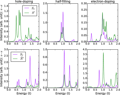
Figure S1: Comparison between ${S^{\prime}}$ and 3-spin Green’s functions $S_{3}$ and between $\tilde{N^{\prime}}$ and 2-spin Green’s functions $S_{2}$ calculated using exact diagonalization and following the Eqs. (8) and (II.2) from the main text of the paper and Eqs. (Appendix B: UCL approximation for the $t-J$ model) and (Appendix B: UCL approximation for the $t-J$ model). Top (bottom) panels show spectra for the $\pi-\sigma$ ($\pi-\pi$) polarization setups, see main text of the paper for further details. Left, middle, and right panels show RIXS spectra calculated for $n=0.83$, $n=1$, and $n=1.17$ electron fillings, respectively. The spectra are summed over all momenta along the nodal direction and along the $k_{y}=0$ direction that are accessible in RIXS and on a 12-site cluster used in the exact diagonalization calculations and weighted with the RIXS form factors, i.e.: $S^{\prime}(\omega)=\sum_{\bf q}|{W}_{\bf\pi\!-\!\sigma}|^{2}{S^{\prime}}({\bf q},\omega)$, $\tilde{N^{\prime}}(\omega)=\sum_{\bf q}|{W}_{\bf\pi\!-\!\pi}|^{2}\tilde{N^{\prime}}({\bf q},\omega)$, $S_{2}(\omega)=\sum_{\bf q}|{W}_{\bf\pi\!-\!\pi}|^{2}S_{2}({\bf q},\omega)$, and $S_{3}(\omega)=\sum_{\bf q}|{W}_{\bf\pi\!-\!\sigma}|^{2}S_{3}({\bf q},\omega)$. The intensity scale is different on each panel (it is chosen in such a way that each of the 6 spectra can be well visible) and the elastic response has been removed.

These equations show that in the second order of the UCL expansion we obtain two terms. The first ones contain only the spin operators and correspond to the ‘2-spin’

$$S_{2}({\bf q},\omega)= \frac{z^{2}J^{2}}{N\Gamma^{2}}\sum_{f}\Big{|}\Big{\langle}f\Big{|}\sum_{\bf k}\gamma_{{\bf q}-{\bf k}}{\bf S}_{\bf k}{\bf S}_{{\bf k}-{\bf q}}\Big{|}i\Big{\rangle}\Big{|}^{2}$$

$$\times\delta(\omega+E_{i}-E_{f}),$$ (35)

and ‘3-spin’ Green’s functions

$$S_{3}({\bf q},\omega)= \frac{z^{2}J^{2}}{L^{2}\Gamma^{2}}\sum_{f}\Big{|}\Big{\langle}f\Big{|}\sum_{{\bf k},{\bf k^{\prime}}}\gamma_{{\bf k^{\prime}}+{\bf k}-{\bf q}}S^{z}_{\bf k^{\prime}}$$

$$\times{\bf S}_{\bf k}{\bf S}_{-{\bf k^{\prime}}-{\bf k}+{\bf q}}\Big{|}i\Big{\rangle}\Big{|}^{2}\delta(\omega+E_{i}-E_{f}).$$ (36)

The second terms always involve charge excitations below the gap. Since these terms do not contribute at half-filling (due to the constrained Hilbert space without double occupancies), it is expected that at relatively low doping levels, the first terms should be dominant (even though their amplitude scales with $J/\Gamma$ and not with $t/\Gamma$). Hence, we compare the spectra of these first two terms, $S_{2}({\bf q},\omega)$ and $S_{3}({\bf q},\omega)$, in the second order of the UCL expansion with the spectra of $S^{\prime}({\bf q},\omega)$ and $\tilde{N^{\prime}}({\bf q},\omega)$ (cf. Fig. S1) from the Hubbard model. We see that at half-filling $S^{\prime}({\bf q},\omega)$ can be approximated relatively well by the ‘3-spin’ excitations probed by $S_{3}({\bf q},\omega)$ and that $\tilde{N^{\prime}}({\bf q},\omega)$ can be approximated relatively well by the “2-spin” or bi-magnon excitations probed by $S_{2}({\bf q},\omega)$. Most of the discrepancies between these two spectra can be found in the high energy regime and are therefore attributed to the failure of the $t$–$J$ model expansion at higher energies. The electron- and hole-doped cases show much less pronounced agreement, where the projected spin and charge excitations $S^{\prime}({\bf q},\omega)$ and $\tilde{N^{\prime}}({\bf q},\omega)$ also probe the low energy charge excitations below the gap which can give a relatively large contribution in the spectrum.

The prediction that RIXS can probe the “2-spin” and the “3-spin” excitations at half-filling already has been put forward in Refs. Ament2010 ; Bisogni2012a ; Bisogni2012b ; Kourtis2012 ; Igarashi2012a ; Igarashi2012b in the case of the Heisenberg model, consistent with our UCL expansions for the Hubbard and $t$–$J$ models. Note that usually the Greens functions containing the ‘2-spin’ and the ‘3-spin’ operators are referred to as probing the ‘two-magnon’ and the ‘three-magnon’ spectrum, though this terminology may be used loosely in this context. Finally, the fact that the charge dynamical structure factor for the half-filled Hubbard model probes the ‘two-magnon’ spectrum also has been discussed in the context of nonresonant Raman scattering (cf. Ref. [Morr1996, ; Devereaux2007, ; Lin2012, ]).

Appendix C: Visualization of the final state configurations

Fig. S2 shows the dominant Cu $L$-edge RIXS process in the cross-polarized channel in hole language. The hole in the $3d^{*}$ orbital on a particular site ${\bf j}$ in the initial state of RIXS is transferred via the dipole operator $D$ into the $2p$ orbital on the same site ${\bf j}$ with a non-uniquely defined spin in the intermediate state of RIXS due to spin-orbit coupling in the core. This is transferred back via the dipole operator $D^{{\dagger}}$ to the $d$ orbital on the same site ${\bf j}$ with a spin flip in the final state compared to the initial state of the RIXS process. While we demonstrate this process on a single site ${\bf j}$ in real space, in reality a coherent superposition of such excitations are created with phase factors $e^{\imath{\bf q}{\bf j}}$; this leads to a well-defined, single spin flip with momentum ${\bf q}$ in the final state of RIXS, i.e. RIXS is sensitive to the spin dynamical structure factor ${S}({\bf q},\omega)$.

Fig. S3 shows the dominant Cu $L$-edge RIXS process in the parallel-polarized channel in hole language. The hole in the $3d^{*}$ orbital on a particular site ${\bf j}$ in the initial state of RIXS is transferred via the dipole operator $D$ into the $2p$ orbital on the same site ${\bf j}$ with a well defined spin in the intermediate state. In the intermediate state a “shakeup” happens, which creates a “2-spin” and/or charge excitation in the final state. While this process is shown on a single site ${\bf j}$ (and its neighbors) in real space, in reality a coherent superposition of such excitations is created with a phase factor $e^{\imath{\bf q}{\bf j}}$; leading to a “2-spin” or charge excitation created with momentum ${\bf q}$ in the final state, i.e. RIXS has some sensitivity to $\tilde{N^{\prime}}({\bf q},\omega)$, which unfortunately have no simple analog in the standard two-particle charge response function.

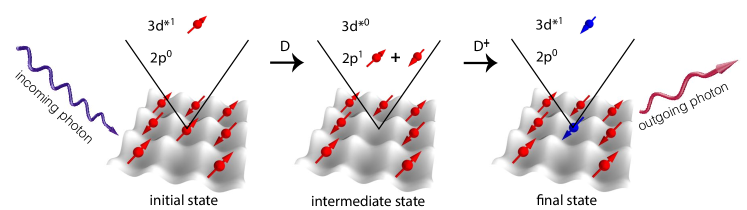
Figure S2: A cartoon picture of the dominant Cu $L$-edge RIXS process in the cross-polarized ‘channel’.

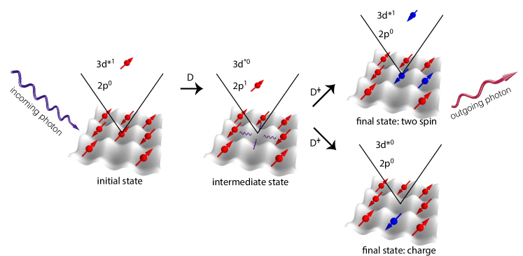
Figure S3: A cartoon picture of the dominant Cu $L$ edge RIXS process in the parallel-polarized ‘channel’.

References

- (1) L. J. P. Ament et al., Review of Modern Physics 83, 705 (2011).
- (2) J. Schlappa et al., Physical Review Letters 103, 047401 (2009).
- (3) L. Braicovich et al., Physical Review Letters 102, 167401 (2009).
- (4) M. Guarise et al., Phys. Rev. Lett. 105, 157006 (2010).
- (5) L. Braicovich et al., Phys. Rev. Lett. 104, 077002 (2010).
- (6) J. Schlappa et al., Nature 485, 82 (2012).
- (7) M. Le Tacon et al., Nature Physics 7, 725 (2011).
- (8) M. P. M. Dean et al., Phys. Rev. Lett. 110, 147001 (2013).
- (9) M. P. M. Dean et al., Nature Materials 12, 1019 (2013).
- (10) M. P. M. Dean et al., Phys. Rev. B 88, 020403 (2013).
- (11) M. Le Tacon et al., Phys. Rev. B 88, 020501 (2013).
- (12) K. Ishii et al., Nature Communications 5, 3714 (2014).
- (13) W. S. Lee et al., Nature Physics 10, 883 (2014).
- (14) M. P. M. Dean et al., Phys. Rev. B 90, 220506 (2014).
- (15) M. Guarise et al., Nature Communications 5, 5760 (2014).
- (16) M. Minola et al., Phys. Rev. Lett. 114, 217003 (2015).
- (17) S. Wakimoto et al., Phys. Rev. B 91, 184513 (2015).
- (18) T. P. Devereaux and R. Hackl, Rev. Mod. Phys. 79, 175 (2007).
- (19) C. J. Jia et al., Nature Communications 5, 3314 (2014).
- (20) C. J. Jia et al., New Journal of Physics 14, 113038 (2012).
- (21) Y. Wang, C. J. Jia, B. Moritz, and T. P. Devereaux, Phys. Rev. Lett. 112, 156402 (2014).
- (22) L. J. P. Ament et al., Phys. Rev. Lett. 103, 117003 (2009).
- (23) J. Luo, G. T. Trammell, and J. P. Hannon, Phys. Rev. Lett. 71, 287 (1993).
- (24) F. M. F. de Groot, P. Kuiper, and G. A. Sawatzky, Phys. Rev. B 57, 14584 (1998).
- (25) M. van Veenendaal, Phys. Rev. Lett. 96, 117404 (2006).
- (26) M. W. Haverkort, Phys. Rev. Lett. 105, 167404 (2010).
- (27) P. Marra, K. Wohlfeld, and J. van den Brink, Phys. Rev. Lett. 109, 117401 (2012).
- (28) L. J. P. Ament, F. Forte, and J. van den Brink, Phys. Rev. B 75, 115118 (2007).
- (29) V. Bisogni et al., Phys. Rev. B 85, 214527 (2012).
- (30) V. Bisogni et al., Phys. Rev. B 85, 214528 (2012).
- (31) J.-I. Igarashi and T. Nagao, Phys. Rev. B 85, 064421 (2012).
- (32) L. J. P. Ament and J. van den Brink, ArXiv:1002.3773 (2010).
- (33) D. Benjamin, I. Klich, and E. Demler, Phys. Rev. Lett. 112, 247002 (2014).
- (34) F. C. Zhang and T. M. Rice, Phys. Rev. B 37, 3759 (1988).
- (35) R. B. Lehoucq, D. C. Sorensen, and C. Yang, ARPACK User s Guide: Solution of Large-Scale Eigenvalue Problems with Implicitly Restarted Arnoldi Methods (SIAM, Philadelphia, 1998).
- (36) H. A. Van der Vorst, SIAM J. Sci. Stat. Comput. 13, 631 (1992).
- (37) E. Dagotto, Rev. Mod. Phys. 66, 763 (1994).
- (38) K. Wohlfeld, S. Nishimoto, M. W. Haverkort, and J. van den Brink, Phys. Rev. B 88, 195138 (2013).
- (39) At this resonance, the intermediate state is an element of a subspace with no hole on the core-hole site.
- (40) J. van den Brink and M. van Veenendaal, EPL (Europhysics Letters) 73, 121 (2006).
- (41) F. Forte, L. J. P. Ament, and J. van den Brink, Phys. Rev. B 77, 134428 (2008).
- (42) S. Kourtis, J. van den Brink, and M. Daghofer, Phys. Rev. B 85, 064423 (2012).
- (43) J.-I. Igarashi and T. Nagao, Phys. Rev. B 85, 064422 (2012).
- (44) D. K. Morr, A. V. Chubukov, A. P. Kampf, and G. Blumberg, Phys. Rev. B 54, 3468 (1996).
- (45) N. Lin, E. Gull, and A. J. Millis, Phys. Rev. Lett. 109, 106401 (2012).