Transient Growth in Stochastic Burgers Flows

Abstract

This study considers the problem of the extreme behavior exhibited by solutions to Burgers equation subject to stochastic forcing. More specifically, we are interested in the maximum growth achieved by the “enstrophy” (the Sobolev $H^{1}$ seminorm of the solution) as a function of the initial enstrophy $\mathcal{E}_{0}$, in particular, whether in the stochastic setting this growth is different than in the deterministic case considered by Ayala & Protas (2011). This problem is motivated by questions about the effect of noise on the possible singularity formation in hydrodynamic models. The main quantities of interest in the stochastic problem are the expected value of the enstrophy and the enstrophy of the expected value of the solution. The stochastic Burgers equation is solved numerically with a Monte Carlo sampling approach. By studying solutions obtained for a range of optimal initial data and different noise magnitudes, we reveal different solution behaviors and it is demonstrated that the two quantities always bracket the enstrophy of the deterministic solution. The key finding is that the expected values of the enstrophy exhibit the same power-law dependence on the initial enstrophy $\mathcal{E}_{0}$ as reported in the deterministic case. This indicates that the stochastic excitation does not increase the extreme enstrophy growth beyond what is already observed in the deterministic case.

Keywords: stochastic Burgers equation; extreme behavior; enstrophy; singularity formation; Monte Carlo

1 Introduction and Problem Statement

Many open problems related to nonlinear partial differential equations (PDEs) of mathematical physics concern the extreme behavior which can be exhibited by their solutions. By this we mean, among other, questions concerning the maximum possible growth of certain norms of the solution of the PDE. From the physics point of view, these norms measure different properties of the solution, such as generation of small scales in the case of the Sobolev norms. The question of the maximum possible growth of solution norms is also intrinsically linked to the problem of existence of solutions to PDE problems in a given functional space. More specifically, the loss of regularity of a solution resulting from the formation of singularities usually manifests itself in an unbounded growth of some solution norms in finite time, typically referred to as “blow-up”. While problems of this type remain open for many important PDEs of mathematical physics, most attention has been arguably given to establishing the regularity of the three-dimensional (3D) Navier-Stokes equations [19], a problem which has been recognized by the Clay Mathematics Institute as one of its “millennium problems” [21]. Analogous questions also remain open for the 3D inviscid Euler equation [24]. The problem we address in the present study is how the transient growth of solutions to certain nonlinear PDEs is affected by the presence of noise represented by a suitably defined stochastic forcing term in the equation. More specifically, the key question is whether via some interaction with the nonlinearity and dissipation present in the system such stochastic forcing may enhance or weaken the growth of certain solution norms as compared to the deterministic case. In particular, in the case of systems exhibiting finite-time blow-up in the deterministic case it is interesting to know whether noise may accelerate or delay the formation of a singularity, or perhaps even prevent it entirely [22]. These questions are of course nuanced by the fact that they may be considered either for individual trajectories or in suitable statistical terms. We add that transient growth in linear stochastic systems is well understood [31] and here we focus on the interaction of the stochastic forcing with a particular type of nonlinearity.

Since this study is ultimately motivated by questions concerning extreme behavior in hydrodynamic models, we will focus our attention on the simplest model used in this context, namely, the one-dimensional (1D) stochastic Burgers equation defined on a periodic interval $[0,1]$

$$\partial_{t}u+{\frac{1}{2}\partial_{x}u^{2}}-\nu\partial_{x}^{2}u =\zeta \text{in}\ (0,T]\times(0,1),$$ (1a)

$$u(t,0)=u(t,1)\ \text{and}\ \partial_{x}u(t,0) =\partial_{x}u(t,1)\qquad \text{for}\ t\in[0,T],$$ (1b)

$$u(0,x) =g(x) \text{for}\ x\in(0,1),$$ (1c)

in which $T>0$ represents the length of the time window of interest, $\nu>0$ is the viscosity coefficient (hereafter we will use $\nu=0.001$) and $g\in H^{1}_{p}(0,1)$ is the initial condition, where $H^{1}_{p}(0,1)$ denotes the Sobolev space of periodic functions defined on $(0,1)$ with square integrable derivatives and the norm given by [1]

$$\|u(t,\cdot)\|_{H_{p}^{1}}^{2}=\int_{0}^{1}|u(t,x)|^{2}+|\partial_{x}u(t,x)|^{2}\,dx.$$ (2)

For simplicity, we will denote the time-space domain $D:=(0,T]\times(0,1)$ (“$:=$” means “equal to by definition”). In equation (1a) the stochastic forcing is given by a random field $\zeta(t,x)$, $(t,x)\in D$. Therefore, at any point $(t,x)$ our solution becomes a random variable $u={u(t,x;\omega)}$ for $\omega$ in some probability space $\Omega$. We add that, while for other systems, such as e.g., the Schrödinger equation [18], one may also consider multiplicative noise, for dissipative models of the type (1a) one typically studies additive noise. The reason is that, as argued in [22, Section 5.5.2], multiplicative noise tends to have effect similar to dissipative terms, so if the equation already involves such a term, then no major qualitative changes in the solution behavior can be expected.

A common approach to modelling stochastic excitation in PDE systems is to describe it in terms of Gaussian noise white both in time and space, and associated with an infinite-variance Wiener process. However, as will be discussed in Section 2, such a noise model does not ensure that individual solutions are well defined in the Sobolev space $H^{1}_{p}$ and is therefore not suitable for the problem considered here. Thus, for the remainder of this paper, we shall restrict our attention to the case where $\zeta$ is the derivative of a Wiener process with finite variance, which is the most “aggressive” stochastic excitation still leaving problem (1) well-posed in $H^{1}_{p}$ (precise definition is deferred to Section 2). We add that the stochastic Burgers equation is related to the Kardar-Parisi-Zhang equation, which has received some attention in the literature [30, 38], except that the latter is typically studied in the presence of noise which is white both in space and in time.

We now briefly summarize important results from the literature relevant to the stochastic Burgers equation. The existence and uniqueness of solutions has been proven in [11, 28] for the problem posed on the real line and in [42, 27] for a bounded domain with Dirichlet boundary conditions. In all cases, solutions can be regarded as continuous $L^{p}$-valued random processes. For the bounded domain (the case which we are interested in), convergence of numerical schemes has been established in [2] for the finite-difference approaches and in [12] for Galerkin approximations. However, in both cases only Dirichlet boundary conditions were considered. The case with the periodic boundary conditions has been recently considered in [29] for a larger class of Burgers-type equations and an abstract numerical scheme.

There exists a large body of literature devoted to investigations of stochastically forced Burgers equation used as a model for three-dimensional (3D) turbulence. Below we mention a few landmark studies and refer the reader to the survey paper [10] for additional details and references. The majority of these investigations aimed to characterize the solutions obtained in statistical equilibrium, attained by averaging over sufficiently long times, in terms of properties of the stochastic forcing. Given the motivation to obtain insights about actual turbulent flows, the main quantities of interest in these studies were the scaling of the energy spectrum, evidence for intermittency in the anomalous scaling of the structure functions and the statistics of $\partial_{x}u$, such as the tails (exponential vs. algebraic) of its probability density function [15, 16, 46]. Remarkably, some of these results were also established with mathematical rigour [13]. The aforementioned quantities were also studied in flows evolving from stochastic initial data [25]. In this context we mention the investigations [45, 44] which focused on the statistics of shock waves in the limit of vanishing viscosity $\nu$. As regards technical developments, a number of interesting results were obtained using optimization-based instanton formulations [38, 9, 26]. While most of earlier investigations of stochastic problems in hydrodynamics were concerned with the properties of the statistically steady state obtained in the long-time limit [35], the focus of the present investigation is fundamentally different, as here we explore extreme forms of the transient behavior under stochastic excitation. In other words, instead of studying the behavior in a time-averaged sense, we seek to understand how the worst-case scenarios are affected by stochastic forcing. The idea that stochastic excitation could act to re-establish global well-posedness in a system exhibiting a finite-time blow-up in the deterministic setting has been considered for some time, although more progress has been made on the related problem of restoring uniqueness [22]. The rationale for why noise might prevent the formation of singularities is that in some situations blow-up may require a simultaneous occurrence of certain conditions (phenomena) and this coincidence may be disrupted by stochastic excitations. There are in fact some model problems where such mechanism of regularization by noise has been proved to exist, including certain transport equations [22] and some versions of the Schrödinger equation [18]. While there are a few related results available for the 3D Navier-Stokes and Euler equations [23], here we mention the studies [3, 4] where it was shown that singularity formation (gradient blow-up) in the inviscid Burgers equation can be prevented by a certain stochastic excitation of the associated Lagrangian particle trajectories.

However, there are also cases in which noise may amplify formation of singularities. For example, the paper [20] deals with the stochastic inviscid Burgers equation in which the stochastic forcing is periodic in the spatial coordinate and represented by white noise in time. The authors show that introducing noise increases the number of shocks present in the stochastic solution as compared to the deterministic case. In particular, this means that solutions are discontinuous (at almost all times $t$) and belong in a space of locally integrable functions. We will return to these results at the end of the paper.

For deterministic systems which exhibit blow-up, singularity formation is typically signalled by unbounded growth of certain Sobolev norms [33]. This growth can often be estimated using bounds obtained with methods of functional analysis and even for problems which are globally well-posed, such as the viscous Burgers equation [34], it is important to understand how much these Sobolev norms can grow depending on the “size” of the initial data as this can provide valuable insights concerning the sharpness of the corresponding estimates. These issues are at the heart of the recently undertaken research program aiming to probe the sharpness of fundamental estimates on the growth of quadratic quantities in hydrodynamic models [5, 6, 7]. These estimates are of two types, namely, concerning the instantaneous growth (i.e., the rate of change at a fixed instant of time) and growth over finite time windows. Important progress has also been made on some related questions in the context of the 3D Navier-Stokes problem [37, 8] which is in fact what has motivated this research program.

Figure 1: (a) Space-time evolution of the solution $u(t,x)$ and (b) history of the enstrophy ${{\mathcal{E}}(u(t))}$ in a solution of the deterministic Burgers equation with an extreme initial condition $\tilde{g}_{\mathcal{E}_{0},T}$. In figure (a) the level sets of $u(t,x)$ are plotted with increments of 0.1.

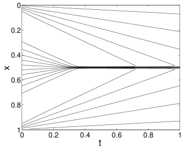
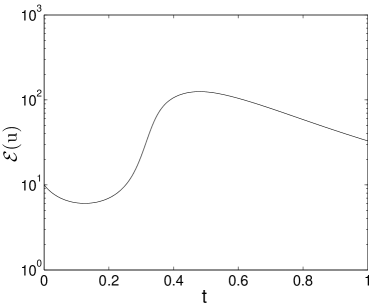
For Burgers equation the key quantity of interest is the $H^{1}$ seminorm of the solution referred to as enstrophy

$${{\mathcal{E}}(u(t))}:=\frac{1}{2}\int_{0}^{1}|\partial_{x}u(t,x)|^{2}\,dx.$$ (3)

In the deterministic setting ($\zeta\equiv 0$ in (1a)), where Burgers equation is known to be globally well-posed [34], its solutions generically exhibit a steepening of the gradients (driven by the nonlinearity) followed by their viscous dissipation when the linear dissipative term starts to dominate. This behavior is manifested by an initial growth of enstrophy ${{\mathcal{E}}(u(t))}$, which peaks when the solution $u(t,\cdot)$ builds up the steepest front, followed by its eventual decay to zero. As a point of reference, we illustrate this generic behavior in Figure 1 in which the results were obtained by solving system (1) with $\zeta\equiv 0$, $T=1$ and an “extreme” initial condition $\tilde{g}_{\mathcal{E}_{0},T}$ designed to produce a maximum enstrophy growth over $[0,1]$ for a given ${\mathcal{E}}_{0}:={{\mathcal{E}}(\tilde{g}_{\mathcal{E}_{0},T})}$ [5] (the numerical approach used to obtain the results in Figure 1 and the construction of the extreme initial data $\tilde{g}_{\mathcal{E}_{0},T}$ will be described in Sections 3 and 4, respectively). Although the evolution shown in Figure 1 corresponds to a special choice of the initial data, it is qualitatively similar to the generic case. While the best estimate for the finite-time growth of enstrophy predicts $\max_{t\geq 0}{\mathcal{E}}(t)\leq C\,{\mathcal{E}}_{0}^{3}$ for some $C>0$, where ${\mathcal{E}}_{0}:={\mathcal{E}}(0)={\frac{1}{2}\int_{0}^{1}|\partial_{x}g(x)|^{2}\,dx}$, computational evidence was presented in [5] that this estimate may not in fact be sharp and the largest possible growth of enstrophy actually scales as $\max_{t\geq 0}{\mathcal{E}}(t)\sim{\mathcal{E}}_{0}^{3/2}$. Given the relation between the growth of their Sobolev norms and the extreme (in particular, singular) behavior of solutions, it is important to understand whether this growth of enstrophy may be affected by stochastic excitation. The main goal of the present study is therefore to address this question in the context of the 1D Burgers equation. In order to do so, we will have to use a more “aggressive” form of stochastic excitation than was used in earlier investigations of the stochastic Burgers problem where the forcing acted mostly on large scales. While this question is clearly of mathematical nature, in the absence of any theoretical estimates available for the effect of noise, either instantaneously or in finite time, on the growth of Sobolev norms of solutions to evolutionary stochastic PDEs, we will address it here through a series of carefully designed and executed computational experiments. The intention is that these results may motivate and guide further mathematical analysis of this problem. We add that, with the exception of the study [18], which concerned the stochastic Schrödinger equation, to the best of our knowledge there have been no computational studies of such problems.

1.1 Summary of the Main Results

The main question we address here is how the growth of the enstrophy described by stochastic system (1), both in terms of individual trajectories and statistical properties, depends on the properties of the noise term in equation (1a), in particular, whether this growth is enhanced or weakened in comparison to the growth observed in the deterministic system [5], cf. Figure 1. We have made the following observations:

• individual samples of the stochastic solution tend to exhibit a larger growth of enstrophy than the deterministic solution,

• when the noise magnitude is sufficiently large relative to the initial enstrophy $\mathcal{E}_{0}$, the dynamics of individual sample solutions is entirely dominated by noise and exhibits little effect of the initial data,

• when the noise magnitude is small relative to the initial enstrophy, individual solution samples can be regarded as “perturbations” of the deterministic evolution with enstrophy growth dependent on $\mathcal{E}_{0}$,

• in statistical terms, the enstrophy growth $\max_{t\in[0,T]}{\mathcal{E}}({t})$ in the deterministic case provides

  • an upper bound for the growth of the enstrophy of the expected value $\max_{t\in[0,T]}{\mathcal{E}}(\mathbb{E}[u(t)])$, and

  • a lower bound for the growth of the expected value of the enstrophy $\max_{t\in[0,T]}\mathbb{E}[{\mathcal{E}}(u(t))]$,

• when the noise magnitude increases proportionally to the initial enstrophy $\mathcal{E}_{0}$, the same growth of the expected value of the enstrophy is observed as in the deterministic case; this leads us to conclude that inclusion of stochastic forcing does not trigger any new mechanisms of enstrophy amplification.

The remainder of this paper is divided as follows: in the next section we describe our model of noise and discuss some properties of the stochastic solutions; the numerical approach is introduced briefly in Section 3, whereas the computational results are presented and discussed in Section 4; conclusions are presented in Section 5.

2 Structure of the Stochastic Forcing and Properties of the Solution

As is customary in the standard theory of stochastic partial differential equations (SPDEs), we write the stochastic Burgers equation (1a) in the differential form [36]

$$du=\left(\nu\partial^{2}_{x}u{-}\frac{1}{2}\partial_{x}u^{2}\right)\,dt+\sigma\,dW,$$ (4)

where $\zeta=\sigma\frac{dW}{dt}$ in which $\sigma>0$ is a constant and $W(t)$ is a cylindrical Wiener process. One can consider different notions of solution of system (1). Due to the lack of smoothness of the noise term, we do not expect to obtain solutions defined in the classical sense (i.e., solutions continuously differentiable with respect to the independent variables). One can, however, define the notion of a mild solution as in [42]

$$u(t)=e^{tA}g{-}\frac{1}{2}\int_{0}^{t}e^{(t-s)A}\partial_{x}u^{2}\,ds+\sigma\int_{0}^{t}e^{(t-s)A}\,dW(s),$$ (5)

where $A:=\nu\partial_{x}^{2}$ and the action of $e^{tA}$ on $L^{2}$ functions is determined by the identity

$$e^{tA}\,e^{2\pi ikx}=e^{-4\pi^{2}\nu tk^{2}}\,e^{2\pi ikx},\qquad k\in\mathbb{Z},\quad x\in[0,1].$$

We remark that other notions of solution also exist, for example, the notion of a weak solution as defined in [2].

As regards the structure of the stochastic forcing, $\{W(t)\}_{t\geq 0}$ is formally given by

$$W(t)=\sum_{j\in\mathbb{N}}\gamma_{j}\beta_{j}(t)\chi_{j},$$ (6)

where $\{\beta_{j}(t)\}_{j\in\mathbb{N}}$ are i.i.d standard Brownian motions, $\{\chi_{j}\}_{j\in\mathbb{N}}$ form a trigonometric orthonormal basis, i.e.,

$${\chi_{0}=1,\quad\chi_{2j}=\sqrt{2}\cos(2\pi jx),\quad\chi_{2j-1}=\sqrt{2}\sin(2\pi jx),\qquad j>0}$$ (7)

and $\{\gamma_{j}\}_{j\in\mathbb{N}}$ are scaling coefficients. When $\forall j$ $\gamma_{j}=1$, $W$ is an infinite-variance Wiener process and $\zeta$ is Gaussian noise white in both time and space, which is commonly used in investigations of SPDEs. However, this choice is not suitable for the present study, since we are interested here in the effects of stochastic excitation on the enstrophy, cf. (3), and, as is demonstrated below, this quantity is in fact not defined for the Gaussian noise white in space.

Suppose $u$ is a mild solution satisfying equation (5) with an infinite-variance noise $W$. For convenience, let $\phi_{k}:=e^{2\pi ikx}$, $k\in\mathbb{Z}$, denote elements of the orthonormal Fourier basis. We now study each of the terms appearing on the right-hand side of (5).

Analysis of first term: under the assumption that $g\in L_{p}^{2}$, so that $\sum_{k\in\mathbb{Z}}|\hat{g}_{k}|^{2}<\infty$, we have that $e^{tA}g\in H_{p}^{1}$ (actually $H_{p}^{\ell}$ for any $\ell\geq 0$), since

$$\|e^{tA}g\|_{H_{p}^{1}}^{2}=\sum_{k\in\mathbb{Z}}\frac{1+4\pi^{2}k^{2}}{e^{4\nu\pi^{2}k^{2}t}}|\hat{g}_{k}|^{2}<\infty$$

which is true because the exponentials dominate all other factors.

Analysis of second term: under the assumption that $u\in L^{2}(\Omega,C([0,T],L_{p}^{4}))$, so that $u^{2}\in L^{2}(\Omega,C([0,T],L_{p}^{2}))$, we can write

$$u^{2}=\sum_{k\in\mathbb{Z}}\hat{y}_{k}\phi_{k}\quad\text{with}\quad\sum_{k\in\mathbb{Z}}\|\hat{y}_{k}\|_{L^{2}(\Omega,C([0,T],\mathbb{C}))}^{2}=\sum_{k\in\mathbb{Z}}\mathbb{E}\left[\sup_{0\leq t\leq T}|\hat{y}_{k}|^{2}\right]<\infty,$$

so that

$$\partial_{x}u^{2}=2\pi i\sum_{k\in\mathbb{Z}}k\hat{y}_{k}\phi_{k}$$

and

$$\int_{0}^{t}\frac{1}{2}e^{(t-s)A}\partial_{x}u^{2}\,ds=\sum_{k\in\mathbb{Z}}\left[\int_{0}^{t}\frac{2\pi i}{2}ke^{-4\nu\pi^{2}k^{2}(t-s)}\hat{y}_{k}(s)\,ds\right]\phi_{k};$$

now each of the coefficients in the sum above can be bounded as

$$\left|\int_{0}^{t}\frac{2\pi i}{2}ke^{-4\nu\pi^{2}k^{2}(t-s)}\hat{y}_{k}(s)\,ds\right| \leq\int_{0}^{t}\pi ke^{-4\nu\pi^{2}k^{2}(t-s)}ds\sup_{0\leq t\leq T}|\hat{y}_{k}|$$

$$=\frac{1}{\nu\pi k}\left(1-e^{-8\nu\pi^{2}k^{2}t}\right)\sup_{0\leq t\leq T}|\hat{y}_{k}|\leq\frac{1}{\nu\pi k}\sup_{0\leq t\leq T}|\hat{y}_{k}|,$$

so that the second term in (5) is also in $H_{p}^{1}$ with

$$\left\|\int_{0}^{t}\frac{1}{2}e^{(t-s)A}\partial_{x}u^{2}\,ds\right\|^{2}_{L^{2}(\Omega,H_{p}^{1})} \leq\sum_{k\in\mathbb{Z}}(1+4\pi^{2}k^{2})\left\|\frac{1}{\nu\pi k}\sup_{0\leq t\leq T}|\hat{y}_{k}|\right\|_{L^{2}(\Omega,\mathbb{C})}^{2}$$

$$=\sum_{k\in\mathbb{Z}}\frac{1+4\pi^{2}k^{2}}{\nu^{2}\pi^{2}k^{2}}\|\hat{y}_{k}\|_{L^{2}(\Omega,C([0,T],\mathbb{C}))}^{2}<\infty$$

which follows from the summability of $\|\hat{y}_{k}\|^{2}$.

Analysis of third term: writing it in terms of a Fourier series

$$\sigma\int_{0}^{t}e^{(t-s)A}\,dW(s)=\sum_{k\in\mathbb{Z}}\hat{W}_{k}(t)\,\phi_{k},$$

we obtain (for $k>0$ with the cases $k=0$ and $k<0$ handled similarly)

$$\hat{W}_{k}(t)=\sigma\int_{0}^{t}e^{-4\nu\pi^{2}k^{2}(t-s)}\left(\frac{\sqrt{2}}{2}d\beta_{2k}(s)-i\frac{\sqrt{2}}{2}d\beta_{2k}(s)\right)$$

which is a random variable with the second moment given by

$$\|\hat{W}_{k}(t)\|_{L^{2}(\Omega,\mathbb{C})}^{2}=\sigma^{2}\int_{0}^{t}e^{-8\nu\pi^{2}k^{2}(t-s)}\,ds=\frac{\sigma^{2}}{8\nu\pi^{2}k^{2}}\left(1-e^{-8\nu\pi^{2}k^{2}t}\right);$$

from this we see that the third term is in $L^{2}$ but not in $H_{p}^{1}$, as for any $t>0$ we have

$$\left\|\sigma\int_{0}^{t}e^{(t-s)A}\,dW(s)\right\|_{L^{2}(\Omega,H_{p}^{1})}^{2} =\sum_{k\in\mathbb{Z}}(1+4\pi^{2}k^{2})\|\hat{W}_{k}\|_{L^{2}(\Omega,\mathbb{C})}^{2}$$

$$=\frac{\sigma^{2}}{8\nu\pi^{2}}\sum_{k\in\mathbb{Z}}\frac{1+4\pi^{2}k^{2}}{k^{2}}(1-e^{-8\nu\pi^{2}k^{2}t})=\infty.$$

We therefore conclude that while the first two terms on the right-hand side of (5) are in $H_{p}^{1}$ (and hence also in $L^{2}$), the third one is only in $L^{2}$ and not in $H_{p}^{1}$. Thus, for any $t>0$, $u(t)$, being the left-hand side of (5), is in $L^{2}$ but not in $H_{p}^{1}$, and consequently the enstrophy obtained with Gaussian noise white in space is not well defined.

We shall thus focus on noise representations with $\ell^{2}$-summable coefficients, such as

$$\gamma_{0}=1,\quad\gamma_{2k+1}=\gamma_{2k+2}=\frac{1}{k},\qquad k>0,$$ (8)

so that $W(t)$ has a finite variance, meaning that it is square-integrable in $L^{2}$, i.e., $W(t)\in L^{2}(\Omega,L^{2})$, with the norm

$$\|W(t)\|_{L^{2}(\Omega,L^{2})}^{2}=\sum_{j\in\mathbb{N}}|\gamma_{j}|^{2}\|\beta_{j}(t)\|_{L^{2}(\Omega,\mathbb{C})}^{2}\|\chi_{j}\|_{L^{2}}^{2}=t\sum_{j\in\mathbb{N}}\gamma_{j}^{2}=\left(1+\frac{\pi^{2}}{3}\right)t.$$ (9)

Such a finite-variance Wiener process ensures that the enstrophy is a well-defined quantity. The corresponding term $\zeta$ in equation (1a) will be referred to as the Gaussian colored-in-space noise. We add that a finite-variance Wiener process may also be constructed with scaling coefficients $\{\gamma_{j}\}_{j\in\mathbb{N}}$ decaying a bit less rapidly than indicated in (8), namely as $\gamma_{2k+1}=\gamma_{2k+2}=1/k^{1/2+\epsilon}$ or $\gamma_{2k+1}=\gamma_{2k+2}=(\ln k)^{1+\epsilon}/k$, $k>0$, for some $\epsilon>0$. We tested stochastic actuation with such structure computationally, but in terms of the quantities we are interested in there was no appreciable difference with respect to (8). Therefore, hereafter we will focus on stochastic excitations defined by (8).

3 Numerical Approach

System (1) will be discretized with respect to the three independent variables, namely, the space variable $x$, time $t$ and the stochastic variable $\omega\in\Omega$. Since our numerical approach is fairly standard (similar techniques were employed in [15, 16]), we describe it below only briefly. The approach is then validated in Section 3.1.

Discretization with respect to the space variable $x$ is performed using a spectral approach based on truncated Fourier series. Since the nonlinear term $(1/2)\partial_{x}u^{2}$ is represented as a convolution sum in the Fourier space, it can be evaluated more efficiently in the physical space with a pseudospectral approach based on the Fast Fourier Transforms (FFTs) combined with dealiasing based on the “3/2” rule [14]. We let $K$ denote the discretization parameter equal to the number of Fourier modes, so that $K=\lfloor\frac{M}{3}\rfloor$, where $M$ is the number of grid points in the physical space. To maximize the performance of FFTs, $M$ will be taken to be a large power of 2.

Discretization with respect to the time variable $t$ is performed using a finite-difference approach based on a uniform grid in time. We use a semi-implicit (first-order) Euler method in which the dissipative term is treated implicitly, whereas the nonlinear and the stochastic terms are treated explicitly. We let $N$ denote the discretization parameter representing the number of time steps in the interval $[0,T]$.

Discretization of the stochastic forcing $\zeta$ is performed using a Monte Carlo approach to sample the distribution of the stochastic variable $\omega\in\Omega$. We compute realizations of the stochastic solution for a sequence of noise samples which, consistently with the spectral approach to discretization in space, are represented as random realizations of the coefficients $\{\beta_{j}(t)\}_{j\in\mathbb{N}}$ in Fourier expansion (6). The expected values of the Fourier coefficients of the solution can then be approximated using the average estimator [36, Section 4.4]. We let $S$ denote the discretization parameter representing the number of samples.

For $k=0,\ldots K$, $n=0,\ldots,N$ and $s=1,\ldots,S$, we let $\hat{u}^{K,N,S}_{k,n,s}$ denote the $s$-th realization of the $k$-th Fourier mode of $u=u(t,x;\omega)$ at time $t_{n}=\frac{n}{N}T$. We recall that we wish to compute the enstrophy of the solution, defined in (3). In the stochastic setting, there are two distinct quantities of interest: one can either consider the enstrophy of the expected value of the stochastic solution, or the expected value of the enstrophy of the stochastic solution. Estimates of both these quantities can be obtained using the expressions

$$\mathcal{E}(\mathbb{E}[u(t_{n})]) \approx\sum_{k=1}^{K}4\pi^{2}k^{2}\left|\frac{1}{S}\sum_{s=1}^{S}\hat{u}^{K,N,S}_{k,n,s}\right|^{2},$$ (10a)

$$\mathbb{E}[\mathcal{E}(u(t_{n}))] \approx\sum_{k=1}^{K}4\pi^{2}k^{2}\frac{1}{S}\sum_{s=1}^{S}\left|\hat{u}^{K,N,S}_{k,n,s}\right|^{2}.$$ (10b)

These two quantities (and also their estimates) are related via Jensen’s inequality [36]

$$\mathcal{E}(\mathbb{E}[u(t)])\;\leq\;\mathbb{E}[\mathcal{E}(u(t))].$$ (11)

The reason for also including $\mathcal{E}(\mathbb{E}[u(t)])$ in our analysis is that quantities related to averaged (mean) fields are often employed in statistical theories of turbulent flows [41, 17], e.g., in the context of the so-called Reynolds-Averaged Navier-Stokes equations.

Our choice of the Monte Carlo approach to noise sampling is motivated by its well-understood convergence properties and straightforward implementation. While more modern approaches, such as polynomial chaos expansions, may in principle achieve faster convergence, they suffer from much higher computational complexity (at least polynomial in the number of random variables, which is $N(2K+1)$ for our discretization). Moreover, the nonlinear term will have a rather complicated expression in the polynomial orthonormal basis, a challenge which does not arise only in linear problems [36, Chapter 9]. We also remark that the low-order of the time-integration scheme in our approach is justified by the need to simultaneously account for stochastic excitation which is not a smooth function of time.

3.1 Validation

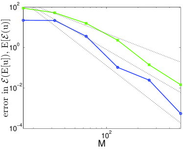
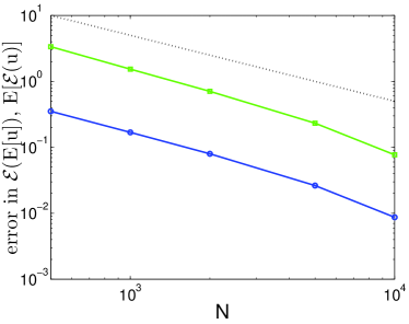
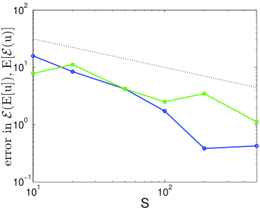
Since a rigorous convergence proof of the numerical approach presented above would be outside the scope of the present study, we limit ourselves to showing computational evidence that this approach is indeed convergent. Given that there are three numerical parameters, $M$, $N$ and $S$, this is achieved by studying solutions to problem (5) as each of the three parameters is refined with the other two held fixed. In each case we monitor the difference between approximations of the quantities (10a) and (10b) and their values corresponding to the reference solution obtained with the finest discretization: $K=341=\lfloor\frac{1024}{3}\rfloor$ dealiased complex Fourier modes (corresponding to $M=1024$ grid points in the physical space), $N=20,000$ time steps and $S=1000$ Monte Carlo samples. These results, obtained using the initial data $\tilde{g}_{\mathcal{E}_{0},T}$ with ${\mathcal{E}}_{0}=10$ and $T=1$, are presented in Figures 2a,b,c. In Figure 2a, showing the effect of the spatial discretization parameter $M$ with $N=20,000$ and $S=1000$ fixed, we see that the rate of decrease of the error increases with $M$, which is an indication of spectral convergence. In Figure 2b, showing the effect of the temporal discretization parameter $N$ with $M=1024$ and $S=1000$ fixed, we observe linear convergence of the errors for both quantities of interest. Finally, in Figure 2c, showing the effect of the stochastic sampling parameter $S$ with $M=1024$ and $N=20,000$ fixed, we see that the rate of convergence of the error is about $1/2$. We thus conclude that the proposed numerical approach is convergent, with the expected rates of convergence [36], as each of the three numerical parameters is refined. The numerical parameters characterizing the reference solution described above represent a reasonable trade-off between accuracy and computational cost, and were used to obtain the results presented in Section 4. To simplify the notation, we will use the symbol $u=u(t,x;\omega)$ to represent the solution obtained numerically with these parameter values.

Figure 2: Errors in the numerical approximations of $\mathcal{E}(\mathbb{E}[u(T)])$ (blue lines and circles) and $\mathbb{E}[\mathcal{E}(u(T))]$ (green lines and squares) as functions of (a) the spatial discretization parameter $M$ with $N=20,000$ and $S=1000$ fixed, (b) the temporal discretization parameter $N$ with $M=1024$ and $S=1000$ fixed and (c) the sampling discretization parameter $S$ with $M=1024$ and $N=20,000$ fixed. The initial data used was $\tilde{g}_{\mathcal{E}_{0},T}$ with $\mathcal{E}_{0}=10$ and $T=1$, and the errors are evaluated with respect to the reference solutions computed with $M=1024$, $N=20,000$ and $S=1000$. The dashed black lines correspond to the power laws (a) $CM^{-2}$, $CM^{-3}$, and $CM^{-4}$ , (b) $CN^{-1}$, and (c) $CS^{-1/2}$ with suitably adjusted constants $C$.

4 Computational Results

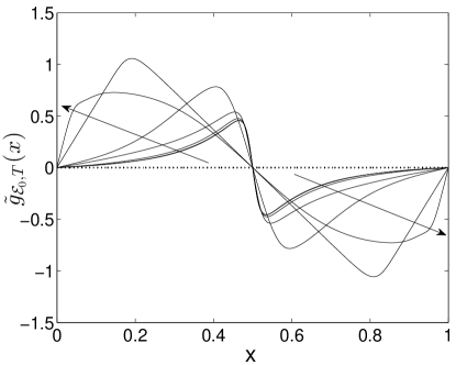
In this section we use the numerical approach introduced above to study the effect of the stochastic excitation with the structure described in Section 2 on the enstrophy growth in the solutions of Burgers equation. More specifically, we will address the question formulated in Introduction, namely, whether or not the presence of noise can change the maximum growth of enstrophy observed in the deterministic setting in [5]. We will do so by studying how the growth of the two quantities, $\mathcal{E}(\mathbb{E}[{u}])$ and $\mathbb{E}[\mathcal{E}({u})]$ introduced in Section 3, is affected by the stochastic excitation as a function of the initial enstrophy $\mathcal{E}_{0}=\frac{1}{2}\int_{0}^{1}|\partial_{x}g(x)|^{2}\,dx$. Given time intervals of different length $T$, we will solve system (1) subject to optimal initial condition $\tilde{g}_{\mathcal{E}_{0},T}$ which is designed to produce the largest possible growth of enstrophy at time $T$ for all initial data in $H^{1}_{p}$ with enstrophy $\mathcal{E}_{0}$. The procedure for obtaining such optimal initial data is discussed in [5] and the optimal initial conditions corresponding to $\mathcal{E}_{0}=10$ and different time windows $T$ are shown in Figure 3. We see in this figure that, as $T$ increases, the form of the optimal initial data changes from a “shock wave” to a “rarefaction wave”. We remark that the optimal initial data $\tilde{g}_{\mathcal{E}_{0},T}$ was obtained in the deterministic setting and, as such, might not produce optimal enstrophy growth in the presence of stochastic forcing. To probe such possibility, we also conducted tests with other initial conditions in the form $g(x)=A\sin(2\pi kx)$, where $k=1,2,\dots$ and $A\in\mathbb{R}$ was chosen to satisfy the condition ${\mathcal{E}}(g)={\mathcal{E}}_{0}$. We note that for different values of $k$ such initial conditions represent mutually orthogonal “directions” in the space $H_{p}^{1}(0,1)$. However, in all such cases the observed growth of $\mathcal{E}(\mathbb{E}[{u}])$ and $\mathbb{E}[\mathcal{E}({u})]$ was always inferior to the growth obtained with the initial data $\tilde{g}_{\mathcal{E}_{0},T}$, hence these results are not reported here.

Figure 3: Optimal initial conditions $\tilde{g}_{\mathcal{E}_{0},T}(x)$ for $\mathcal{E}_{0}=10$ and $T$ ranging from $10^{-3}$ to $1$ [5] (arrows indicate the directions of increase of $T$).

In the subsections below we first recall some properties of the extreme enstrophy growth in the deterministic setting and then discuss the effect of the noise on the enstrophy growth over time and globally as a function of $\mathcal{E}_{0}$.

4.1 Deterministic Case Revisited

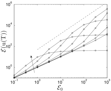
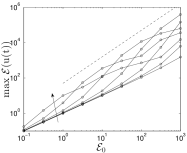
The deterministic case will serve as a reference and here we summarize some key facts about the corresponding maximum enstrophy growth. The reader is referred to studies [5, 37, 40, 39] for additional details. As illustrated in Figure 1, a typical behavior of the solutions to Burgers equation involves a steepening of the initial gradients, which is manifested as a growth of enstrophy, followed by their dissipation when the enstrophy eventually decreases. The key question is how the enstrophy at some fixed time $\mathcal{E}(T)$, or the maximum enstrophy $\max_{t\in[0,T]}\mathcal{E}(t)$, depend on the initial enstrophy $\mathcal{E}_{0}$. While the sharpest available analytical estimate predicts $\max_{t\geq 0}\mathcal{E}(t)\leq C\,\mathcal{E}_{0}^{3}$ for large $\mathcal{E}_{0}$, it was found in [5] that under the most extreme circumstances the actual system evolution does not saturate this upper bound producing instead $\max_{t\in[0,T]}\mathcal{E}(t)\sim\mathcal{E}_{0}^{3/2}$. These results are illustrated in Figure 4a,b, where we can also see that for very short evolution times growth only linear in $\mathcal{E}_{0}$ is observed (this is because for small $\mathcal{E}_{0}$ the solutions do not have enough time to produce sharp gradients). Since for increasing $\mathcal{E}_{0}$ the maximum growth of enstrophy is achieved for different $T$, the power-law behavior is obtained by taking a maximum of $\mathcal{E}(T)$ or $\max_{t\in[0,T]}\mathcal{E}(t)$ with respect to $T$ (represented in Figures 4a,b as “envelopes” of the curves corresponding to different values of $T$).

Figure 4: Dependence of (a) the enstrophy $\mathcal{E}(T)$ at a final time $T$ and (b) the maximum enstrophy $\max_{t\in[0,T]}\mathcal{E}(t)$ on the initial enstrophy $\mathcal{E}_{0}$ for the optimal initial data $\tilde{g}_{\mathcal{E}_{0},T}$ with $T$ in the range from $10^{-3}$ to $1$. Arrows indicate the direction of increasing $T$ and the dashed lines correspond to the power law $C\,\mathcal{E}_{0}^{3/2}$.

4.2 Effect of Noise on Time Evolution

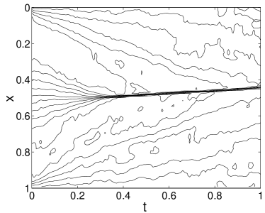
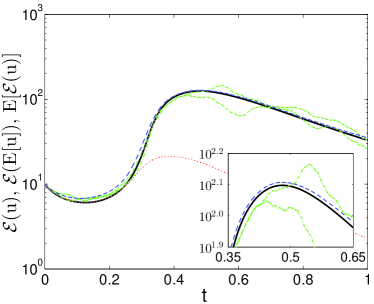
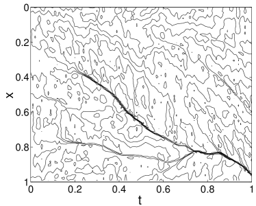
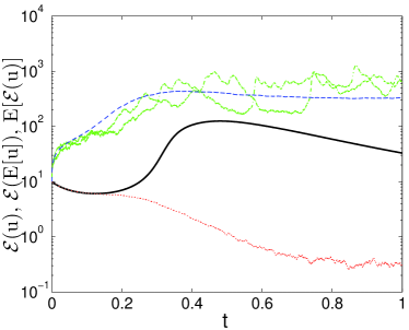
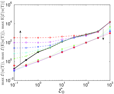
We now analyze the effect of noise, both in terms of individual trajectories and in the statistical sense, as a function of time during the evolution starting from the optimal initial data $\tilde{g}_{\mathcal{E}_{0},T}$ with enstrophy $\mathcal{E}_{0}=10$ and a fixed final time $T=1$. Stochastic solutions corresponding to “small” noise magnitude $\sigma^{2}=10^{-2}$ and “large” noise magnitude $\sigma^{2}=1$ are illustrated in Figures 6 and 6, respectively. The individual stochastic trajectories are shown as functions of space and time in Figures 6a and 6a. We see that in the small-noise case the effect of the stochastic excitation is to gradually change the position of the “shock wave” (cf. Figures 1a and 6a). In the large-noise case the steep gradient region from the initial data is gone and is replaced with spontaneously appearing and interacting shocks which move in a largely structureless field (Figure 6a). The corresponding evolutions of the enstrophy of some sample stochastic solutions $\mathcal{E}({u(t;\omega_{s})})$, $s=1,2$, the expected value of the enstrophy $\mathbb{E}[\mathcal{E}({u(t)})]$ and the enstrophy of the expected value of the solution $\mathcal{E}(\mathbb{E}[{u(t)}])$ are shown in Figures 6b and 6b for the two noise levels where they are also compared to the enstrophy evolution $\mathcal{E}(t)$ in the deterministic case. We see that the enstrophy of the sample stochastic solutions tends to exceed the enstrophy of the deterministic solution for most, albeit not all, times. As regards the relation of the the expected value of the enstrophy $\mathbb{E}[\mathcal{E}({u(t)})]$ and the enstrophy of the expected value of the solution $\mathcal{E}(\mathbb{E}[{u(t)}])$ to the enstrophy $\mathcal{E}(t)$ in the deterministic case, the following relationship is observed

$$\mathcal{E}(\mathbb{E}[{u(t)}])\ \leq\ \mathcal{E}(t)\ \leq\ \mathbb{E}[\mathcal{E}({u(t)})],\quad t>0$$ (12)

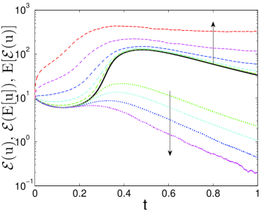
for both noise levels. While the relation between $\mathcal{E}(\mathbb{E}[{u(t)}])$ and $\mathbb{E}[\mathcal{E}({u(t)})]$ is a consequence of Jensen’s inequality (11), the fact that these two quantities in fact bracket the enstrophy of the deterministic solution uniformly in time appears rather non-obvious. This conclusion is further elaborated in Figure 7 where we show the time evolution of the three quantities from (12) for increasing noise levels. We see that the difference between $\mathcal{E}(\mathbb{E}[{u(t)}])$ and $\mathbb{E}[\mathcal{E}({u(t)})]$ increases with the noise magnitude $\sigma^{2}$, such that at large noise levels the enstrophy of the expected value of the solution exhibits no growth at all. The fluctuations evident in $\mathcal{E}(\mathbb{E}[{u(t)}])$ corresponding to the largest noise level are a numerical artefact resulting from an insufficient number of Monte Carlo samples, due to the fact that increased noise levels slow down the convergence of the Monte Carlo approach.

Figure 5: [Small noise case: $\sigma^{2}=10^{-2}$] (a) Sample stochastic solution ${u(t,x)}$ as a function of space and time (the level sets are plotted with the increments of $0.1$), (b) evolution of enstrophy of two sample stochastic solutions $\mathcal{E}({u(t;\omega_{s})})$, $s=1,2$, (green dash-dotted lines), the enstrophy of the deterministic solution $\mathcal{E}(t)$ (black solid line), the expected value of the enstrophy $\mathbb{E}[\mathcal{E}({u(t)})]$ (blue dashed line) and the enstrophy of the expected value of the solution $\mathcal{E}(\mathbb{E}[{u(t)}])$ (red dotted line). The initial data used was $\tilde{g}_{\mathcal{E}_{0},T}$ with $\mathcal{E}_{0}=10$ and $T=1$. The inset in figure (b) shows details of the evolution during the subinterval $[0.35,0.65]$.

Figure 6: [Large noise case: $\sigma^{2}=1$] (see previous figure for details).

Figure 7: The expected value of the enstrophy $\mathbb{E}[\mathcal{E}({u(t)})]$ (dashed lines), the enstrophy of the expected value of the solution $\mathcal{E}(\mathbb{E}[{u(t)}])$ (dotted lines) and the enstrophy $\mathcal{E}(t)$ of the deterministic solution (thick solid line) as functions of time for the initial condition $\tilde{g}_{\mathcal{E}_{0},T}$ with $\mathcal{E}_{0}=10$, $T=1$ and different noise levels $\sigma^{2}$ in the range from $10^{-2}$ to $1$ (the direction of increase of $\sigma^{2}$ is indicated by arrows).

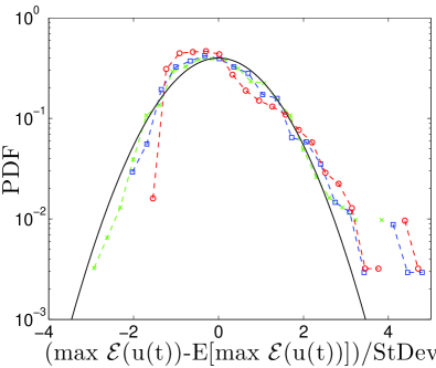
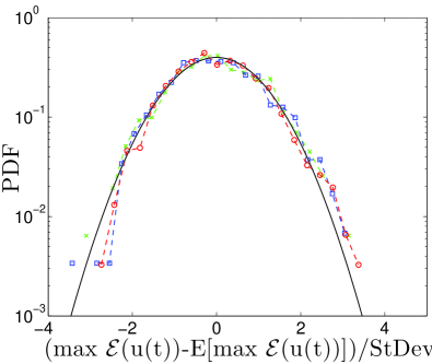
The distributions of the maximum enstrophy values $\max_{t\geq 0}{\mathcal{E}}(u({t;\omega}))$ corresponding to different stochastic realizations $\omega$ of the noise are shown for the cases with ${\mathcal{E}}_{0}=10,10^{3}$ and $T=1$ as probability distribution functions (PDFs) in Figures 8(a,b). It is evident from these figures that the PDFs are non-Gaussian and, in particular, are asymmetric with heavy, possibly algebraic, tails characterizing values of $\max_{t\geq 0}{\mathcal{E}}({u(t,\omega)})$ larger than $\mathbb{E}[{\max_{t\geq 0}\mathcal{E}(u(t))}]$. However, it is also clear that the deviation from the Gaussian behavior is significantly smaller in the larger enstrophy case (Figure 8(b)) than in the lower enstrophy case (Figure 8(a)). This deviation also tends to increase with the noise magnitude $\sigma^{2}$.

Figure 8: Normalized PDFs of the maximum enstrophy values $\max_{t\geq 0}{\mathcal{E}}(u(t,\omega))$ for the cases with the initial condition $\tilde{g}_{\mathcal{E}_{0},T}$ with $T=1$ and (a) $\mathcal{E}_{0}=10$, (b) $\mathcal{E}_{0}=10^{3}$. The noise levels $\sigma^{2}$ are equal to $10^{-2}$ (green lines and crosses), $10^{-1}$ (blue lines and squares) and $1$ (red lines and circles). To obtain these plots, $S=10^{5}$ samples were collected in each case and sorted into $30$ equispaced bins. The solid lines correspond to the standard Gaussian distributions.

4.3 Global Effect of Noise on Enstrophy Growth for Varying $\mathcal{E}_{0}$

In this section we analyze how the diagnostic quantities

$$\mathbb{E}[\mathcal{E}({u(T)})], \mathcal{E}(\mathbb{E}[{u(T)}]),$$ (13a)

$$\max_{t\in[0,T]} \mathbb{E}[\mathcal{E}({u(t)})], \qquad\max_{t\in[0,T]} \mathcal{E}(\mathbb{E}[{u(t)}])$$ (13b)

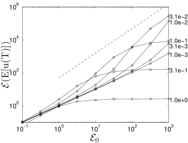
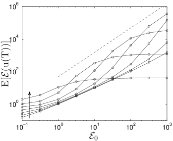
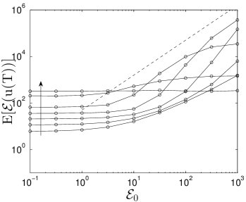
for some given $T$ depend on the initial enstrophy $\mathcal{E}_{0}$ and whether the presence of the stochastic excitation modifies the power-law dependence of the quantities (13b) on $\mathcal{E}_{0}$ as compared to the deterministic case (cf. Section 4.1). We will do this in two cases, namely, when for different values of the initial enstrophy ${\mathcal{E}}_{0}$ the noise level $\sigma^{2}$ is fixed and when it is proportional to ${\mathcal{E}}_{0}$. Concerning the first case, Figures 9a and 9b show the dependence of the quantities (13a) and (13b) with $T=1$ on $\mathcal{E}_{0}$ for different fixed noise levels. The quantities $\mathcal{E}(\mathbb{E}[{u(T)}])$ and $\mathbb{E}[\mathcal{E}({u(T)})]$ for different time horizons $T$ are plotted as functions of $\mathcal{E}_{0}$ for small and large noise levels, respectively, in Figures 11 and 11. These plots are therefore the stochastic counterparts of Figure 4 representing the deterministic case [5]. We see that with a fixed $T$ both $\mathcal{E}(\mathbb{E}[{u(T)}])$ and $\mathbb{E}[\mathcal{E}({u(T)})]$ saturate at a level depending on the noise magnitude $\sigma^{2}$ (Figure 9a). Analogous behavior is observed for a fixed noise level and increasing time intervals in Figures 11 and 11, from which we can also conclude that when we maximize the quantities $\mathcal{E}(\mathbb{E}[{u(T)}])$ and $\mathbb{E}[\mathcal{E}({u(T)})]$ over all considered values of $T$, then the resulting quantity will scale proportionally to $\mathcal{E}_{0}^{3/2}$, which is the same behavior as observed in the deterministic case (Figure 4). The process of maximizing with respect to $T$ is represented schematically in Figures 11 and 11 as “envelopes” of the curves corresponding to different values of $T$. Regarding the behavior of the quantities (13b), for every noise level we observe a transition from a noise-dominated behavior, where $\max_{t\in[0,T]}\mathbb{E}[\mathcal{E}({u(t)})]$ does not increase with $\mathcal{E}_{0}$ when $\mathcal{E}_{0}$ is small, to a nonlinearity-dominated regime in which $\max_{t\in[0,T]}\mathbb{E}[\mathcal{E}({u(t)})]$ grows with $\mathcal{E}_{0}$ (Figure 9b). In the latter regime, corresponding to large values of $\mathcal{E}_{0}$ and whose lower bound is an increasing function of the noise magnitude, we observe that for sufficiently large $\mathcal{E}_{0}$ the growth of the quantity $\max_{t\in[0,T]}\mathbb{E}[\mathcal{E}({u(t)})]$ in all cases approaches the growth observed in the deterministic case [5].

Figure 9: (a) The values at $T=1$ and (b) the maximum values attained in $[0,T]$ of the expected value of the enstrophy $\mathbb{E}[\mathcal{E}({u(t)})]$ (dashed lines), the enstrophy of the expected value of the solution $\mathcal{E}(\mathbb{E}[{u(t)}])$ (dotted lines) and the enstrophy $\mathcal{E}(t)$ of the deterministic solution (thick solid line) as functions of the initial enstrophy $\mathcal{E}_{0}$ for the initial condition $\tilde{g}_{\mathcal{E}_{0},T}$ with $\mathcal{E}_{0}=10$, $T=1$ and different noise levels $\sigma^{2}$ in the range from $10^{-2}$ to $1$ (the direction of increase of $\sigma^{2}$ is indicated by arrows)

Figure 10: [Small noise case: $\sigma^{2}=10^{-2}$] Dependence of (a) the enstrophy of the expected value of the solution $\mathcal{E}(\mathbb{E}[{u(T)}])$ and (b) the expected value of the enstrophy $\mathbb{E}[\mathcal{E}({u(T)})]$ on the initial enstrophy $\mathcal{E}_{0}$ using the initial condition $\tilde{g}_{\mathcal{E}_{0},T}$ with $T$ varying from $10^{-3}$ to $1$. In (a) the values of $T$ are marked near the right edge of the plot, whereas in (b) the direction of increasing $T$ is indicated with an arrow. The dashed lines correspond to the power law $C\,\mathcal{E}_{0}^{3/2}$.

Figure 11: [Large noise case: $\sigma^{2}=1$] (see previous figure for details).

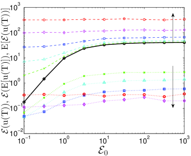
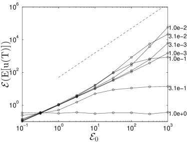
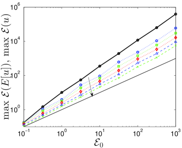
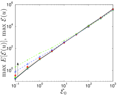
Since the results presented above show no evidence of the effect of noise on the dependence of the quantities (13) on $\mathcal{E}_{0}$ when $\mathcal{E}_{0}$ grows while the noise magnitude stays fixed, to close this section we consider the case in which the noise magnitude is proportional to $\mathcal{E}_{0}$, i.e.,

$$\sigma^{2}=C_{\sigma}\,\mathcal{E}_{0},$$ (14)

for a range of different constants $C_{\sigma}$. The quantities (13b) obtained in this way are shown in Figures 12a and 12b. As regards the dependence of the quantity $\max_{t\in[0,T]}\mathcal{E}(\mathbb{E}[{u(t)}])$ on $\mathcal{E}_{0}$, in Figure 12a we observe a superlinear growth which is however slower than $\mathcal{E}_{0}^{3/2}$ characterizing the deterministic case (in fact, from the data it is not entirely obvious if this dependence is strictly in the form of a power law). Concerning the quantity $\max_{t\in[0,T]}\mathbb{E}[\mathcal{E}({u(t)})]$, Figure 12b indicates that while for small $\mathcal{E}_{0}$ it is larger than $\max_{t\geq 0}\mathcal{E}(t)$ obtained in the deterministic case, in the limit of $\mathcal{E}_{0}\rightarrow\infty$ it reveals the same growth as in the deterministic case, that is, proportional to $\mathcal{E}_{0}^{3/2}$ with approximately the same constant prefactor.

Figure 12: Dependence of (a) the maximum enstrophy of the expected value of the solution $\max_{t\in[0,T]}\mathcal{E}(\mathbb{E}[{u(t)}])$ and (b) the maximum expected value of the enstrophy $\max_{t\in[0,T]}\mathbb{E}[\mathcal{E}({u(t)})]$ on the initial enstrophy $\mathcal{E}_{0}$ using the initial conditions $\tilde{g}_{\mathcal{E}_{0},T}$ and with noise magnitudes proportional to $\mathcal{E}_{0}$, cf. (14), with $C_{\sigma}$ in the range from $10^{-3}$ to $10^{-1}$ (arrow indicate the direction of increase of $C_{\sigma}$). The parameter $T$ is chosen to maximize $\max_{t\in[0,T]}\mathcal{E}(\mathbb{E}[{u(t)}])$ in (a) and $\max_{t\in[0,T]}\mathbb{E}[\mathcal{E}({u(t)})]$ in (b). The thick black solid line corresponds to the quantity $\max_{t\in[0,T]}\mathcal{E}(t)$ obtained in the deterministic case, whereas the thin black solid line in (a) represents the power law $\mathcal{E}_{0}^{1}$.

5 Discussion and Conclusions

The goal of this study was to test whether a stochastic excitation applied to Burgers equation can affect the maximum growth of enstrophy as a function of the initial enstrophy $\mathcal{E}_{0}$ observed in the deterministic case [5]. In the context of hydrodynamic models based on the Navier-Stokes equation, the enstrophy is a convenient indicator of the regularity of solutions and its growth is inherently related to the problem of finite-time singularity formation [19]. In the stochastic problem considered here, there are two relevant quantities related to the enstrophy, namely, the expected value of the enstrophy $\mathbb{E}[\mathcal{E}(u(t))]$ and the enstrophy of the expected value of the solution $\mathcal{E}(\mathbb{E}[u(t)])$. They are related to each other via Jensen’s inequality (11). In the set-up of our problem we allowed for the most “aggressive” form of the stochastic excitation which still ensures that the two quantities are well defined (cf. Section 2). The numerical discretization was carefully designed based on the Monte Carlo sampling.

The effect of the noise was found to depend on the relation between its magnitude $\sigma^{2}$ and the “size” of the initial data as measured by the initial enstrophy $\mathcal{E}_{0}$. When the noise magnitude is large, the stochastic excitation obscures the intrinsic dynamics and any dependence of the diagnostic quantities (13) on $\mathcal{E}_{0}$ is lost. Therefore, the relevant regime is when the noise magnitude is “modest” relative to the initial enstrophy $\mathcal{E}_{0}$, so that the stochastic excitation can be regarded as a “perturbation” of the deterministic dynamics. We observe that the two quantities $\mathbb{E}[\mathcal{E}(u(t))]$ and $\mathcal{E}(\mathbb{E}[u(t)])$ provide, respectively, upper and lower bounds on the enstrophy $\mathcal{E}(t)$ in the deterministic case, cf. (12), with the bounds becoming tighter as the noise magnitude vanishes (Figure 7). The fact that the deterministic enstrophy ${\mathcal{E}}(t)$ is “bracketed” by $\mathbb{E}[\mathcal{E}(u(t))]$ and $\mathcal{E}(\mathbb{E}[u(t)])$ appears to be a new, though not entirely unexpected, finding. The latter case, with the enstrophy of the expected value of the solution $\mathcal{E}(\mathbb{E}[u(t)])$ being lower than the deterministic enstrophy $\mathcal{E}(t)$, can be therefore interpreted in terms of the stochastic excitation having the effect of an increased dissipation of the expected value of the solution.

The non-Gaussian PDFs of the normalized maximum enstrophy $\max_{t\geq 0}{\mathcal{E}}({u(t,\omega)})$ in Figures 8(a,b) indicate the likelihood of events when larger-than-average enstrophy maxima are achieved, although this property becomes less pronounced as the enstrophy ${\mathcal{E}}_{0}$ of the initial condition grows. This can be interpreted to mean that as the magnitude of the nonlinear effects increases, the transient evolution becomes less susceptible to stochastic excitation. We note that non-Gaussian PDFs of solution derivatives $\partial_{x}u$ in stochastic Burgers flows were also reported and analyzed in [15, 16, 46, 25] (since in those studies the PDFs were computed for a different quantity, the actual shapes of the distributions and their dependence on parameters were different).

As regards the expected value of the enstrophy, we observed in Figure 12a that in the limit $\mathcal{E}_{0}\rightarrow\infty$ the quantity $\max_{t\geq 0}\mathbb{E}[\mathcal{E}(u(t))]$ exhibits the same dependence on $\mathcal{E}_{0}$ as in the deterministic case, i.e., it remains proportional to $\mathcal{E}_{0}^{3/2}$, even for the noise magnitude increasing proportionally to $\mathcal{E}_{0}$. Thus, this demonstrates that the stochastic excitation does not damp the maximum growth of enstrophy as a function of the initial enstrophy $\mathcal{E}_{0}$. This observation is further reinforced by the PDFs of $\max_{t\geq 0}{\mathcal{E}}({u(t,\omega)})$ shown in Figures 8(a,b) which are skewed towards values larger than $\mathbb{E}[{\max_{t\geq 0}\mathcal{E}(u(t))}]$, but approach the Gaussian distribution as ${\mathcal{E}}_{0}$ increases. In the light of the findings reported in [3, 4], where it was shown that a certain stochastic excitation can regularize the inviscid Burgers equation, our result does not appear entirely obvious. It can be however interpreted as a consequence of the robustness of the shock-formation process which is not disturbed by stochastic excitation. If these insights could be extrapolated to the 3D case, one could expect that noise would be less likely to regularize the 3D Navier-Stokes system than the corresponding Euler system.

We note that if we rescale the magnitude of the solution $u$ as $u_{a}=a\,u$ for some $a>0$, then the stochastic Burgers equation (1a) will be left invariant if we simultaneously rescale the time, viscosity and the forcing term as $t_{a}=t/a$, $\nu_{a}=a\,\nu$ and $\zeta_{a}=a^{2}\,\zeta$. Therefore, the limit ${\mathcal{E}}_{0}\rightarrow\infty$ (while keeping $\nu$ fixed) considered in the present study is equivalent to the limit $\nu\rightarrow 0$ (while keeping initial data fixed) which was investigated in other studies [45, 44, 20]. In particular, it was shown in [20] that inclusion of additive noise in the inviscid Burgers equation significantly increases the number of shocks. This results is however not inconsistent with our findings, since it corresponds to stochastic forcing with a finite magnitude, whereas for the problem set-up considered here the limit $\nu\rightarrow 0$ would imply vanishing magnitude (at the quadratic rate) of the forcing term.

A number of related questions remain open. First of all, in the present study we numerically solved the stochastic Burgers equation (1) using the extreme initial data $\tilde{g}_{\mathcal{E}_{0},T}$ which was found in [5] by solving a deterministic variational optimization problem. It is however possible that by solving a corresponding stochastic optimization problem one might obtain initial data $g$ leading to an even larger growth of enstrophy in finite time. While such problems are harder to solve than the deterministic one, they are in principle amenable to solution using stochastic programming methods [43]. We add that this approach would be distinct from the “instanton” formulation [38, 9, 26] which due to the saddle-point approximation is effectively equivalent to solution of a deterministic optimization problem. In a similar spirit, it is equally interesting to obtain rigorous estimates on $d\mathcal{E}/dt$ and $\max_{t\geq 0}\mathcal{E}(t)$ in the stochastic setting in terms of $\mathcal{E}_{0}$ and the properties of noise, thereby generalizing the bounds available for the deterministic case [37, 5]. As regards effects of viscous dissipation, it is well known [32] that the fractional Burgers equation is no longer globally well posed when the fractional dissipation exponent $\alpha<1/2$. It would be therefore interesting to see whether the finite-time blow-up known to occur in this supercritical regime can be mollified by noise. Similar questions concerning the interplay between the stochastic excitation and extreme behavior, including possible singularity formation, also arise in the context of the two-dimensional and three-dimensional Navier-Stokes and Euler equations. Addressing at least some of these issues is one of the goals of the ongoing research program mentioned in Introduction.

References

- [1] R. A. Adams and J. F. Fournier, Sobolev Spaces, Elsevier, 2005.
- [2] A. Alabert and I. Gyöngy, On numerical approximation of stochastic Burgers’ equation, in From stochastic calculus to mathematical finance, Springer, 2006, 1–15.
- [3] S. Albeverio and O. Rozanova, The non-viscous Burgers equation associated with random position in coordinate space: a threshold for blow up behaviour, Mathematical Models and Methods in Applied Sciences, 19 (2009), 749–767, URL http://www.worldscientific.com/doi/abs/10.1142/S0218202509003607.
- [4] S. Albeverio and O. Rozanova, Suppression of unbounded gradients in an SDE associated with the Burgers equation, Proceedings of the American Mathematical Society, 138 (2010), 241–251, URL http://www.jstor.org/stable/40590613.
- [5] D. Ayala and B. Protas, On maximum enstrophy growth in a hydrodynamic system, Physica D, 240 (2011), 1553–1563.
- [6] D. Ayala and B. Protas, Maximum palinstrophy growth in 2D incompressible flows, Journal of Fluid Mechanics, 742 (2014), 340–367.
- [7] D. Ayala and B. Protas, Vortices, maximum growth and the problem of finite-time singularity formation, Fluid Dynamics Research, 46 (2014), 031404.
- [8] D. Ayala and B. Protas, Extreme vortex states and the growth of enstrophy in 3D incompressible flows, Journal of Fluid Mechanics, 818 (2017), 772–806.
- [9] E. Balkovsky, G. Falkovich, I. Kolokolov and V. Lebedev, Intermittency of Burgers’ Turbulence, Phys. Rev. Lett., 78 (1997), 1452–1455, URL http://link.aps.org/doi/10.1103/PhysRevLett.78.1452.
- [10] J. Bec and K. Khanin, Burgers turbulence, Physics Reports, 447 (2007), 1–66, URL http://www.sciencedirect.com/science/article/pii/S0370157307001457.
- [11] L. Bertini, N. Cancrini and G. Jona-Lasinio, The stochastic Burgers equation, Communications in Mathematical Physics, 165 (1994), 211–232.
- [12] D. Blomker and A. Jentzen, Galerkin approximations for the stochastic Burgers equation, SIAM Journal on Numerical Analysis, 51 (2013), 694–715.
- [13] A. Boritchev, Decaying turbulence in the generalised Burgers equation, Archive for Rational Mechanics and Analysis, 214 (2014), 331–357, URL http://dx.doi.org/10.1007/s00205-014-0766-5.
- [14] C. Canuto, A. Quarteroni, Y. Hussaini and T. A. Zang, Spectral Methods, Scientific Computation, Springer, 2006.
- [15] A. Chekhlov and V. Yakhot, Kolmogorov turbulence in a random-force-driven Burgers equation, Phys. Rev. E, 51 (1995), R2739–R2742, URL http://link.aps.org/doi/10.1103/PhysRevE.51.R2739.
- [16] A. Chekhlov and V. Yakhot, Kolmogorov turbulence in a random-force-driven Burgers equation: Anomalous scaling and probability density functions, Phys. Rev. E, 52 (1995), 5681–5684, URL http://link.aps.org/doi/10.1103/PhysRevE.52.5681.
- [17] P. A. Davidson, Turbulence. An introduction for scientists and engineers, Oxford University Press, 2004.
- [18] A. Debussche and L. D. Menza, Numerical simulation of focusing stochastic nonlinear Schrödinger equations, Physica D, 162 (2002), 131–154.
- [19] C. R. Doering, The 3D Navier-Stokes problem, Annual Review of Fluid Mechanics, 41 (2009), 109–128.
- [20] W. E, K. Khanin, A. Mazel and Y. Sinai, Invariant measures for burgers equation with stochastic forcing, Annals of Mathematics, 151 (2000), 877–960, URL http://www.jstor.org/stable/121126.
- [21] C. L. Fefferman, Existence and smoothness of the Navier-Stokes equation, URL http://www.claymath.org/sites/default/files/navierstokes.pdf, 2000, Clay Millennium Prize Problem Description.
- [22] F. Flandoli, Random Perturbation of PDEs and Fluid Dynamic Models, Lecture Notes in Mathematics, Springer, 2015.
- [23] F. Flandoli, Stochastic Analysis: A Series of Lectures (Eds. R.C. Dalang, M. Dozzi, F. Flandoli and F. Russo), chapter A Stochastic View over the Open Problem of Well-posedness for the 3D Navier-Stokes Equations, 221–246, Birkhäuser, 2015.
- [24] J. D. Gibbon, M. Bustamante and R. M. Kerr, The three–dimensional Euler equations: singular or non–singular?, Nonlinearity, 21 (2008), 123–129.
- [25] T. Gotoh and R. H. Kraichnan, Statistics of decaying Burgers turbulence, Physics of Fluids A, 5 (1993), 445–457, URL http://scitation.aip.org/content/aip/journal/pofa/5/2/10.1063/1.858868.
- [26] T. Grafke, R. Grauer and T. Schäfer, The instanton method and its numerical implementation in fluid mechanics, Journal of Physics A: Mathematical and Theoretical, 48 (2015), 333001, URL http://stacks.iop.org/1751-8121/48/i=33/a=333001.
- [27] I. Gyöngy, Existence and uniqueness results for semilinear stochastic partial differential equations, Stochastic Processes and their Applications, 73 (1998), 271–299.
- [28] I. Gyöngy and D. Nualart, On the stochastic Burgers’ equation in the real line, The Annals of Probability, 27 (1999), 782–802.
- [29] M. Hairer and K. Matetski, Optimal rate of convergence for stochastic Burgers-type equations, 2015, ArXiv:1504:05134.
- [30] M. Hairer, Solving the KPZ equation, Annals of Mathematics, 178 (2014), 559–664.
- [31] J. Kim and T. Bewley, A linear systems approach to flow control, Ann. Rev. Fluid Mech., 39 (2007), 383–417.
- [32] A. Kiselev, F. Nazarov and A. Volberg, Global well-posedness for the critical 2D dissipative quasi-geostrophic equation, Invent. math., 167 (2006), 445–453.
- [33] C. Klein and J.-C. Saut, A numerical approach to blow-up issues for dispersive perturbations of Burgers’ equation, Physica D, 295–296 (2015), 46–65.
- [34] H. Kreiss and J. Lorenz, Initial-Boundary Value Problems and the Navier-Stokes Equations, vol. 47 of Classics in Applied Mathematics, SIAM, 2004.
- [35] S. Kuksin and A. Shirikyan, Mathematics of two-dimensional turbulence, Cambridge University Press, 2012.
- [36] G. J. Lord, C. E. Powell and T. Shardlow, An Introduction to Computational Stochastic PDEs, Cambridge University Press, 2014.
- [37] L. Lu and C. R. Doering, Limits on enstrophy growth for solutions of the three-dimensional Navier–Stokes equations, Indiana University Mathematics Journal, 57 (2008), 2693–2727.
- [38] B. Meerson, E. Katzav and A. Vilenkin, Large deviations of surface height in the Kardar-Parisi-Zhang equation, Phys. Rev. Lett., 116 (2016), 070601, URL http://link.aps.org/doi/10.1103/PhysRevLett.116.070601.
- [39] D. Pelinovsky, Enstrophy growth in the viscous Burgers equation, Dynamics of Partial Differential Equations, 9 (2012), 305–340.
- [40] D. Pelinovsky, Sharp bounds on enstrophy growth in the viscous Burgers equation, Proceedings of Royal Society A, 468 (2012), 3636–3648.
- [41] S. Pope, Turbulent Flows, 1st edition, Cambridge University Press, Cambridge, UK, 2000.
- [42] G. D. Prato, A. Debussche and R. Temam, Stochastic Burgers’ equation, Nonlinear Differential Equations and Applications, 1 (1994), 289–402.
- [43] A. Ruszczyński, Nonlinear Optimization, Princeton University Press, 2006.
- [44] Z.-S. She, E. Aurell and U. Frisch, The inviscid Burgers equation with initial data of brownian type, Communications in Mathematical Physics, 148 (1992), 623–641, URL http://dx.doi.org/10.1007/BF02096551.
- [45] Y. G. Sinai, Statistics of shocks in solutions of inviscid Burgers equation, Communications in Mathematical Physics, 148 (1992), 601–621, URL http://dx.doi.org/10.1007/BF02096550.
- [46] O. Zikanov, A. Thess and R. Grauer, Statistics of turbulence in a generalized random-force-driven Burgers equation, Physics of Fluids, 9 (1997), 1362–1367, URL http://scitation.aip.org/content/aip/journal/pof2/9/5/10.1063/1.869250.